Deep Learning-Based GNN-Attention Framework for Near-Field Channel Modeling and Beamforming in Sixth-Generation Wireless Systems: A Simulation Study

Summary

This work introduces a deep learning framework based on physics for beamforming and near-field channel modeling in sixth-generation wireless systems using Extremely Large Intelligent Metasurfaces. Compared with traditional far-field communication techniques, the proposed method improves energy efficiency, beamforming gain, and spectrum efficiency.

Abstract

The emergence of sixth-generation (6G) networks has driven the development of Extremely Large Intelligent Metasurfaces (XL-IMS) to deliver ultra-high speeds and high spectral efficiency. Nevertheless, classical far-field channels are not applicable to near-field transmission due to spherical-wave propagation and the lack of spatial stationarity, leading to reduced beamforming performance and increased computational complexity. Therefore, the goal of this research is to develop a method for near-field channel modeling and beamforming optimization based on physics-driven deep learning. The proposed solution utilizes a physics-driven spherical wave channel model, along with graph neural networks (GNNs) and attention mechanisms, to capture local spatial relationships between users and the global network. Additionally, an algorithm for learning-based beamforming is proposed to increase the efficiency of energy focusing on near-field users. The performance of the proposed framework is evaluated using realistic propagation scenarios from the DeepMIMO dataset. The simulation results show that the proposed technique yields an achievable rate of 11.6 bps/Hz, a beamforming gain of 28 dB, a spectral efficiency of 10.5 bps/Hz, an energy efficiency of 9.8 bits/Joule, and a signal-to-interference-plus-noise ratio (SINR) of 25 dB. Compared with traditional techniques such as Zero Forcing (ZF), Minimum Mean Square Error (MMSE), Semidefinite Relaxation (SDR), and Alternating Optimization (AO), the proposed scheme improves overall communication performance by approximately 10-15%. These results reveal that integrating near-field channel modeling with GNN-based attention learning can serve as an efficient and accurate beamforming technique for future 6G wireless networks that utilize XL-IMS technology.

Introduction

Interest in beamforming has grown dramatically in recent years. Extreme capacity requirements have become common with the introduction of 6G, driven by growing demand for better connectivity and faster data rates. For effectively guiding signals and improving overall network performance, beamforming is therefore a promising method¹. Conventional wireless communication systems have effectively utilized far-field spatial resources for spatial diversity. An emerging area of study with enormous promise for future wireless communications is near-field beamforming².

Reconfigurable intelligent surfaces (RIS), on the other hand, are particularly interesting because they can overcome some of the propagation issues associated with the mmWave/THz spectrum^3,4. RIS can reflect, refract, and manipulate incoming electromagnetic waves⁵. In this instance, steering the beam in a desirable direction or shape is the main objective, and the RIS can be depicted as altering the radiating source's radiation patterns. For far-field RIS, a number of fundamental topics have been studied over the years^{6,7,8,9,10,11}, including channel estimation, localization, standardization, and passive/active beamforming. This technology enables multiuser communication by focusing beams, which provide a compromise between path loss and penetration, especially in mid-frequency bands like the 10 GHz range¹². Smart interfaces were further developed within communication networks and are currently being studied to improve spatial resolution and communication bandwidth¹³. The higher frequencies and larger antenna apertures during the 5G to 6G transition convert traditional far-field communication scenarios into near-field communication scenarios^14,15.

The near-field region will be important in 6G networks, necessitating research into new near-field techniques¹⁶. Waves must be treated as spherical rather than plane waves to improve electromagnetic wave propagation in near-field technology. This new physical characteristic exhibits a variety of electromagnetic effects, including spatial non-stationarity, beam splitting, tri-polarization, and evanescent waves¹⁷. Because of this, many conventional communication methods might not fully utilize these new physical characteristics or experience severe performance losses in 6G near-field environments¹⁸. A discrepancy between present far-field communication technologies and near-field propagation models can significantly reduce the effectiveness of current far-field techniques in near-field locations¹⁹. In contrast to traditional far-field narrowband systems, new electromagnetic (EM) effects must be accounted for in near-field wideband RIS systems. First, the near-field channel incorporates two angles and distance dimensions due to the spherical wavefront in the near-field spectrum, in contrast to the flat-waveform hypothesis in far-field channel models. Instead of far-field beam navigation, this results in the near-field beam concentrating action^20,21. The phrase "beam splitting effect" refers to the possibility that beams produced at various occurrences will be concentrated at separate locations²².

Unlike the far-field, where electromagnetic (EM) wavefronts are approximated as planar, near-field communications require consideration of spherical wavefront propagation. This characteristic introduces both opportunities and challenges for future wireless networks. By exploiting spherical wavefronts, beam focusing can concentrate signals within a specific spatial region, enabling improved interference suppression and multi-user communication compared with conventional far-field beam steering. However, it also introduces additional design and signal-processing complexities^23,24. Early studies on near-field communications include the work in²⁵, which outlined the differences between near- and far-field regions, key concepts, technical challenges, applications, and codebook-based channel estimation. Subsequently, the author²⁶examined the fundamental distinctions between planar wavefront-based far-field and spherical wavefront-based near-field transmission, focusing on beamforming, channel analysis, system performance, and integration with next-generation technologies. Furthermore, the author²⁷ investigated major challenges in near-field communications, including channel modeling, estimation, beamforming, hardware architecture, and sensing, while summarizing recent advances in these areas.

Recent studies have extensively investigated near-field wireless communications and channel modeling for emerging 6G systems. Comprehensive surveys have examined near-field communication principles, holographic MIMO architectures, channel modeling techniques, signal processing methods, and integrated sensing and communication applications, while also identifying key challenges associated with channel estimation and system design in near-field environments^28,29. To address the beam-splitting effect in RIS-assisted mmWave/THz systems, various solutions have been proposed, including distributed RIS deployment strategies and true time delay (TTD)-assisted RIS architectures. These approaches improve frequency-selective beam control and mitigate beam-splitting degradation; however, they often entail increased deployment costs, greater hardware complexity, or reliance on specialized delay components ^30,31,32.

Beamforming optimization has received considerable attention due to the combined effects of beam focusing and spatial-wideband distortion in extremely large aperture array (ELAA) systems. Existing studies have explored phase-delay focusing methods, TTD-based architectures, and optimization frameworks for holographic metasurface antennas to enhance beamforming gain and mitigate dual-wideband effects^33,34,35,36. Nevertheless, most XL-IMS-related studies continue to rely on far-field plane-wave assumptions, which are inadequate for extremely large apertures. As a result, important near-field characteristics, including spherical wave propagation, spatial non-stationarity, mutual coupling, and distance-dependent beam focusing, are often neglected^37,38. Recently, artificial intelligence techniques have emerged as promising solutions for near-field beamforming and channel optimization in XL-IMS-enabled 6G networks. In particular, meta-learning-based methods have demonstrated strong adaptability and rapid convergence under dynamic wireless conditions with limited training data. These approaches offer significant potential for intelligent near-field communication systems and future autonomous wireless network optimization^39,40.

Existing beamforming techniques largely rely on simplified far-field channel models that fail to capture critical near-field characteristics in ultra-massive structures. Moreover, dataset-driven evaluations in realistic environments, such as DeepMIMO, remain limited, and joint optimization of near-field channel modeling and beamforming for dynamic user scenarios has received insufficient attention. Additionally, computational scalability remains a key challenge for practical XL-IMS-enabled 6G deployments. To address these limitations, this study proposes a unified framework that combines physics-based spherical-wave channel modeling with GNNs and attention mechanisms for near-field beamforming. The proposed framework explicitly accounts for spatial non-stationarity, metasurface interactions, and distance-dependent propagation, and is validated using the DeepMIMO dataset.

The proposed framework integrates physical channel modeling with deep learning to enable accurate near-field channel representation and beamforming optimization for XL-IMS systems. By explicitly modeling spherical-wave propagation and spatial non-stationarity, this study facilitates precise beam focusing while improving energy allocation, beamforming gain, and interference suppression. The framework further incorporates element-wise optimization of metasurface phase responses to enable adaptive beam steering in dense communication environments. Using realistic propagation scenarios from the DeepMIMO dataset, the proposed approach demonstrates improved spectral efficiency, beamforming performance, and computational efficiency, providing a scalable solution for large-scale XL-IMS-enabled 6G communication networks.

Protocol

The proposed framework for Near-Field Channel Modeling and Beamforming in XL-IMS-enabled 6G systems combines physics-based modeling with machine learning optimization to overcome the limitations of conventional far-field approaches. A near-field channel model incorporating spherical-wave propagation and spatial non-stationarity is developed and validated using the DeepMIMO dataset. Channel information is represented as a graph to capture spatial dependencies between metasurface elements and users, and an end-to-end GNN-attention network is employed to learn beamforming weights for near-field beam focusing. Unlike conventional iterative optimization methods, the learning-based framework directly predicts beamforming solutions, reducing computational complexity while maintaining high accuracy and adaptability to dynamic channel conditions. Performance is evaluated in terms of achievable rate, beamforming gain, and energy efficiency, demonstrating superior results compared with traditional far-field beamforming methods. Figure 1 illustrates the overall framework.

The following are the proposed steps:

Step 1: Configure the DeepMIMO environment

The DeepMIMO v3.x platform is first set up through the O1 Outdoor setup that uses 28 GHz of carrier frequency and 100 MHz of bandwidth. In the simulation, the XL-IMS is represented by a 16×16 uniform planar array of 256 reflecting elements, spaced λ/2 apart. The propagation model chosen is a spherical wave with LoS and NLoS paths.

Step 2: Define XL-IMS geometry and user locations

Design the XL-IMS as a 16×16 planar metasurface that comprises 256 reconfigurable reflective elements. The user terminal devices were randomly distributed within the near-field range, from 0.5m to 10m from the XL-IMS, based on the Rayleigh distance criterion.

Step 3: Generate near-field channels using spherical wave propagation

Model the channels between each reconfigurable metasurface element and the user using spherical wave propagation, which considers distance-induced phase variation.

Step 4: Generate near-field channel data

User Terminals were uniformly distributed within the near-field zone (0.5-10 m) from the XL-IMS panel. Both LoS and NLoS propagation paths generated by the DeepMIMO O1 Outdoor Scenario were used to generate the channels.

Step 5: Prepare the dataset for training and testing

The generated dataset comprised 20,000 samples, of which 16,000 (80%) were used for training and 4,000 (20%) for testing.

Step 6: Normalize input features and prepare model inputs

The final stage of the preparation process involved performing Min-Max scaling on all input features, such as channel magnitude, phase, distance, and user coordinates. This process scaled the data and converted it into tensors, which were fed into the GNN-attention network. The model was optimized using the Adam optimizer with a learning rate of 0.001 and 50 epochs.

Step 7: Apply the attention mechanism

Add an attention mechanism to consider global graph information and capture long-range dependencies between graph nodes. This helps the model to focus on important spatial features.

Step 8: Predict beamforming weights

Predict the beamforming weights and phase shift values using GNN-attention embedding. The intricate, laborious, iterative beamforming procedures are replaced by the prediction method.

Step 9: Evaluate performance metrics

To assess how well communication and beamforming are working, calculate KPIs such as the achievable rate, beamforming gain, spectrum efficiency, energy efficiency, and SINR.

Step 10: Compare against benchmark methods

Compare the proposed algorithm to traditional algorithms, including ZF, MMSE, SDR, and AO.

System model definition

The proposed system considers a 6G wireless network enabled by an XL-IMS comprising 256 reconfigurable reflecting elements that control electromagnetic wave propagation through adjustable phase shifts. As users operate in the near-field region, the conventional far-field planar-wave assumption becomes invalid, requiring consideration of spherical-wave propagation, distance-dependent attenuation, and spatial non-stationarity. The boundary between the near- and far-field regions is determined by the Rayleigh distance, which depends on the metasurface size and the carrier wavelength, and marks the transition from spherical wavefront effects to plane-wave propagation. This is described as follows:

 (1)

Here, D is the metasurface size, λ is the wavelength, and R is the Rayleigh distance. A near-field phenomenon occurs in the communication channel when a user is present in a position that is closer to R than its real value. As the signal travels through different metasurface components, it undergoes distinct phase and amplitude variations.

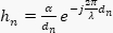
The channel from the n-th meta-surface to the user uses a spherical wave model for near-field propagation, which is represented by the channel coefficient equation as follows:

 (2)

Here, α refers to the path loss parameter, λ refers to the carrier wavelength, and d_n is the user's distance from the component.

In this case, β_n is the path loss factor for the n^th XL-IMS element and can be expressed as β_n = d_n^−α, where α stands for the path loss exponent. It should be noted that d_n is the Euclidean distance from the position of the user to the n^th metasurface element. Channel changes with regard to space are caused by the significant differences in d_n between various meta-surfaces, in contrast to the situation with far-field channels. In general, the channel vector can be explained as follows:

 (3)

The input signal received by the user depends on the phase tuning of the XL-IMS system. Consider θ = [θ₁, θ₂, …., θ_N] to represent the phase shift realized using the metasurface. Then, the input signal can be expressed as:

 (4)

where Φ = diag(e^jθ₁, ….., e^jθ_N) is the transmitted signal, w is the base coding precoding vector, and n stands for noise. The near-field channel vector is defined as h ∈ ℂ^N×1, the diagonal phase-shift matrix of the XL-IMS as Φ ∈ ℂ^N×N, the beamforming vector as x ∈ ℂ^N×1, and the received signal as y ∈ ℂ. The additive noise term is defined as n ∼ CN (0, σ²). These dimensions maintain the mathematical correctness of the formulation.

In this case, ws is the base-station precoding vector that is used to precode the transmitted symbol (s). During performance benchmarking, common digital precoding approaches such as ZF and MMSE are implemented at the base station using similar near-field channel realizations. However, the new approach seeks to optimize the XL-IMS phase-shift matrix (θ) through the GNN-attention learning mechanism.

To concentrate the energy in the near-field region, a design θ where constructive interference occurs, for the user, should be achievable. The beamforming strategy aims to maximize the spectral efficiency or received signal power. Figure 2 describes the architecture of the near-field communication system model based on the XL-IMS approach.

Near-field channel modeling

The proposed XL-IMS-based 6G communication networks near-field model was specifically designed to mimic the propagation conditions near the Rayleigh distance from the metasurface. In the near-field region, propagation is spherical, with changing phase values and non-homogeneous spatial parameters across the metasurface, in contrast to conventional far-field propagation models that assume planar waves. In the current study, a physics-based spherical wave model was used to design an accurate channel impulse response matrix that accounts for the physical locations of both the metasurface elements and user terminals.

Channel representation based on distance

The distance between each metasurface component and the user is a crucial factor in constructing the channel model in the near-field regime. The length p_n among the user locations p_u and the n-th XL-IMS component is provided by:

 (5)

This value varies significantly across the metasurface owing to its extremely large area, leading to unequal propagation times and phase shifts that must be accounted for in the model.

Spherical wave channel model

The channel coefficient between the n-th element and the user is determined using the spherical-wave model described in Equation (2), which captures distance-dependent phase and amplitude variations. For dataset generation and model training, channel coefficients are obtained from the DeepMIMO ray-tracing framework, which incorporates both line-of-sight (LoS) and non-line-of-sight (NLoS) multipath propagation based on realistic environmental structures. From the above, it can construct the channel response matrix from the channel responses for all N meta-surface elements as in Equation (3).

Spatial non-stationarity of near-field channels and model importance

Unlike far-field channels, near-field channels exhibit spatial non-stationarity, where received signals vary across the metasurface, enabling location-dependent beam focusing. This spatial information is embedded in the channel response matrix and is captured by the GNN-attention model. Supplementary Figure 1 illustrates the proposed near-field channel modeling framework for the XL-IMS-based 6G communication system and the generation of realistic channel data for deep learning-based beamforming.

Dataset generation

Data generation was performed using the DeepMIMO framework, which provides realistic ray-tracing-based channel simulations incorporating environmental geometry, spatial consistency, and user mobility. Channel responses for multiple near-field user locations were generated using the O1 outdoor scenario at a carrier frequency of 28 GHz and a bandwidth of 100 MHz. The XL-IMS consisted of 256 uniformly distributed reflective elements, and user locations were selected within the near-field region based on the Rayleigh criterion. Channel coefficients, path gains, and spatial information were extracted using the DeepMIMO Python library. Supplementary Table 1 summarizes the simulation and reproducibility parameters. The model was trained using supervised learning, with channel-state features as inputs and physics-based optimized beamforming weights as target labels.

Input features creation and dataset structure

Next, the raw channel data were converted into features for input to deep learning models. These features included channel response magnitudes and phases as separate components. Other input parameters could also be included depending on the problem requirements. For instance, users' coordinates, distances, and some spatial parameters could also be considered as features. The dataset was split into training and test sets at an 80:20 ratio.

Preparation of the dataset for training

The last step involved normalizing the prepared dataset and converting it into tensors suitable for input into the GNN-attention architecture for training. The training dataset was used to learn the mapping from channel state to the optimal beamforming weights, while the test dataset was used to assess the model's effectiveness. This well-prepared dataset made the learning process easier and more effective. Supplementary Table 2 shows the Dataset Description Details of DeepMIMO.

Feature representation

The feature representation stage transformed complex-valued near-field channel data into a format suitable for deep learning. Channel responses were decomposed into features that capture spatial and propagation characteristics while preserving essential near-field information for learning. Supplementary Figure 2 illustrates the DeepMIMO dataset used in this process. The channel data from the near-field environment were represented as complex numbers h_n, with the real and imaginary components that represent the channel coefficients' phase and amplitude information. To allow for effective use in machine learning algorithms, the coefficients were decomposed into their real (Reh_n) and imaginary (Imh_n) parts. The data could also be represented as the magnitude h_n and the phase of the coefficients ∠h_n.

Spatial feature extraction

In addition to the channel coefficient, spatial features were included to account for the geometric nature of the near-field environment. This included the distance d_n from each metasurface element to the receiver, along with the receiver's coordinates (x, y, z). In this way, the model accounted for the fact that the signal characteristics can depend on the spatial position of the transmitter-receiver pair, a property important to near-field propagation.

Normalization and model input preparation

As a preliminary step before providing the model with its inputs, a normalization process was performed to avoid numerical instability and accelerate convergence. The structured vectors were divided into training and test data sets, denoted by (X_train, X_test). In this way, the inputs were then provided to the GNN and attention models.

Based on the feature representation in Supplementary Figure 2, different kinds of features were used in this dataset, including channel coefficients h_n which indicated the complex signal response of all metasurface elements. Another feature was distance d_n which indicated propagation effects in this case. Although the imaginary and real components provide a numeric description of the signal, the magnitude and phase parts give an explicit description of the signal strength and phase shift, respectively. User position coordinate (x, y, z) was another important feature that enhanced the model's spatial awareness.

Deep learning design using GNN for spatial dependency modeling integrates with a hybrid attention mechanism for global context learning

This learning algorithm was developed to efficiently train the complex near-field XL-IMS channel, with its spatial and propagation characteristics, using GNNs and an attention mechanism. As the metasurface elements are highly correlated with each other and their interactions are non-uniform within the near-field zone, a fully connected network is not appropriate for properly representing the channel. Hence, in this approach, the metasurface is represented as a graph, with each element acting as a node and the interactions between them as edges. The GNN captured localized spatial dependencies between neighboring nodes, while the attention mechanism improved the learning of global dependencies.

Graph representation of XL-IMS

The XL-IMS is created as a graph G = (V, E), with each vertex v_n ∈ V representing one meta-surface element, while edges e_ij ∈ E represent the spatial relations between the elements. Each vertex has a feature vector x_n, which is obtained via the feature representation phase. The adjacency matrix A captures the connectivity among vertices that are close together or within certain distance constraints. Such a graph formulation is used to incorporate the spatial information existing in near-field propagation.

To achieve reproducibility, graph connectivity is determined using the K-Nearest Neighbors approach with k set to 8. Let p_i and p_j represent the location vectors of the i-th and j-th XL-IMS cells, respectively. The distance between any two vertices is measured via the Euclidean metric as follows: d_ij = ||p_i − p_j||². will be an edge between the vertices i and j if vertex j is included in the group of the eight closest neighbors to the vertex i. Therefore, the adjacency matrix is constructed with the following rule: A_ij = 1 if j ∈ N_k(i) and A_ij = 0 otherwise.

In the proposed GNN, updates for each node are calculated based on information from other neighboring nodes. In particular, the propagation of the layer l can be given as follows:

 (6)

where h_i^(l) represents the feature vector of the vertex i in layer l, N(i) is the neighborhood of the vertex i, W^(l) is the learnable weight matrix, and σ(·) symbolizes a nonlinear activation function.

The GNN-attention model consisted of three graph convolutional layers with hidden dimensions set to 128, and Rectified Linear Unit (ReLU) was used as an activation function. Graph generation was performed using the k-nearest neighbors’ method (k=8). Each XL-IMS feature acts as a node, while edges are formed based on the Euclidean distance between adjacent nodes. To extract global spatial dependencies, we used a multi-head self-attention network with 4 heads. The dropout probability was set to 0.3 to prevent overfitting.

Attention mechanism

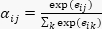
To model long-distance dependencies that existed beyond the local neighborhood range, attention was introduced in the model, which works as follows:

 (7)

where e_ij = LeakyReLU(a^T[Wh_i | Wh_j]) is the importance of the nodes i and j. With this model, one can assign different levels of importance to nodes based on their roles, making it easier for the model to understand the global context across the metasurface. The hybrid framework captures both local and global spatial information, and the learned features are processed through fully connected layers to generate beamforming weights. As shown in Supplementary Figures 3 and 4, the GNN models local spatial dependencies through message passing and feature aggregation, while the attention mechanism captures global interactions among metasurface elements, enabling effective near-field beamforming. Attention weights are computed to quantify the relevance of node pairs, assigning higher importance to more informative interactions. Using these weights, each node aggregates information from all other nodes, enabling the model to capture global dependencies beyond local neighborhoods. The resulting weighted feature fusion generates an optimized feature representation that emphasizes important spatial characteristics while suppressing less relevant information, supporting effective beamforming optimization and energy focusing.

Beamforming optimization

The beamforming optimization stage determined the XL-IMS phase shifts and beamforming weights to focus energy on near-field users. Unlike conventional far-field beam steering, near-field beamforming concentrates energy at specific spatial locations. In the proposed framework, a GNN-attention model learned optimal beamforming parameters directly from channel characteristics, reducing the complexity of iterative optimization methods. The received user signal is given in Equation (4).

Training data were obtained from DeepMIMO for each channel realization, and the corresponding XL-IMS phase shifts were determined using the AO algorithm. The near-field channel matrix h and the XL-IMS phase shift matrix was used to compute the phase shift vector θ by maximizing the received signal power:

 (8)

 (9)

The AO optimizer was run for 100 iterations until it reached the desired convergence threshold of 10⁻⁴. These optimized values served as the training labels for our GNN-attention model. The objective was to achieve constructive interference for effective near-field beam focusing and enhanced received signal power. Instead of conventional optimization methods such as SDR or AO, the problem was solved using a learning-based approach. Specifically, the beamforming optimization problem was approximated by a deep learning model f_Θ(⋅).

Supervised learning was adopted to train the GNN-attention model, with optimal beamforming phase-shift vectors provided by the AO algorithm serving as the training targets. Specifically, let us denote the AO-generated optimal phase-shift vector as θ_AO,i and the network predictions as . Then, the training criterion was formulated as follows:

 (10)

where N is the number of training samples.

Algorithm 1: Near-Field Beamforming using GNN-attention Model is presented in the Supplementary File 1. In this Algorithm, the first step was to set up the system parameters and the DeepMIMO database to create realistic channel conditions. The near-field channel feature for each sample was calculated using the spherical wave model, and the important features, such as channel coefficients and spatial features, were then extracted from the database. The extracted features were converted to a structured form and then represented as a graph, with the metasurface elements as nodes. The deep learning model was generated using GNN layers to capture local spatial dependencies, and an attention mechanism was introduced to learn global dependencies. The deep learning framework was trained using supervised learning with MSE loss between the predicted phase shifts and the AO-generated optimal phase-shift labels.

This implementation was performed with Python and PyTorch. Samples for the DeepMIMO channel were obtained from the O1 outdoor scenario. These channel coefficients were converted into graphs and processed using a GNN with three layers and a multihead attention mechanism. The model was trained using the Adam optimizer with an MSE loss function. This model generated phase shifts and weights for beamforming at near-field users, and the results were evaluated in terms of rate, efficiency, and SINR.

Results

The performance of the introduced Near-Field Channel Modeling and Beamforming framework for XL-IMS in 6G communication networks is assessed using the DeepMIMO Dataset, which offers practical propagation environments and spatially consistent channel data. To configure this dataset, many channel samples representing various user positions in the meta-surface's near-field must be generated. Specifically, this study uses up to 10,000–20,000 samples collected under different propagation conditions and user locations. An 80:20 ratio was used to split these channel samples into 80% for training and 20% for testing. In this sense, the test set assesses the model's ability to generalize, while the training set provides a foundation for learning.

The experimental results demonstrate that the proposed GNN-Attention framework outperforms conventional far-field beamforming and optimization-based methods. By combining spherical-wave channel modeling with deep learning-based spatial feature extraction, the proposed approach achieves higher beamforming gain, spectral efficiency, and energy focusing performance. Performance is evaluated using achievable rate, beamforming gain, and energy efficiency, which measure communication capacity, signal focusing effectiveness, and data transmission efficiency relative to power consumption, respectively.

The proposed method is compared with conventional beamforming techniques, including ZF and MMSE, as well as optimization-based methods such as SDR and AO. While far-field approaches are limited by plane-wave assumptions and perform poorly in near-field XL-IMS environments, optimization methods often incur high computational complexity. In contrast, the GNN-attention framework provides efficient beamforming with lower computational overhead. For a fair comparison, all methods were evaluated using the same DeepMIMO-generated near-field channels, XL-IMS configuration, carrier frequency, user locations, transmission power, and signal-to-noise ratio (SNR) conditions. ZF and MMSE assumed identical channel state information, while SDR and AO were implemented under the same power and phase-shift constraints using standard literature-based parameter settings.

Validation of near-field channel modeling

Benchmark methods, including ZF, MMSE, SDR, and AO, are used to compare the achievable rate performance of the suggested graph neural network-attention-based beamforming model in Figure 3. As SNR increases from 0 to 30 dB, all methods exhibit improved achievable rates; however, the proposed model consistently outperforms the benchmarks. It achieves 2.1 bps/Hz at 0 dB, 7.8 bps/Hz at 15 dB, and 11.6 bps/Hz at 30 dB, exceeding the performance of ZF, MMSE, SDR, and AO across all SNR levels. Table 1 presents a comparison of achievable rates versus SNR.

Figure 4 compares the beamforming gain of the proposed GNN-attention-based model with conventional methods, including ZF, MMSE, SDR, and AO, as a function of user distance in the near-field region. As the user distance increases, the received beamformed signal power decreases due to increased propagation path loss, resulting in a reduction in beamforming gain across all methods. Nevertheless, the proposed GNN-attention framework consistently achieves the highest beamforming gain, attaining approximately 28 dB at 1 m, 25 dB at 4 m, and 22 dB at 7 m, outperforming SDR, AO, MMSE, and ZF across all evaluated distances. These results demonstrate the superior near-field beam-focusing capability and gain retention of the proposed framework, leading to improved beamforming efficiency compared with existing methods.

Performance of GNN-attention learning framework

Figure 5 compares the spectral efficiency of the proposed GNN-attention beamforming scheme with ZF, MMSE, SDR, and AO across SNR values from 0 to 30 dB. Although spectral efficiency increases for all methods with higher SNR, the proposed approach consistently achieves the best performance, reaching 1.8 bps/Hz at 0 dB, 6.8 bps/Hz at 15 dB, and 10.5 bps/Hz at 30 dB, outperforming all benchmark methods. Figure 6 compares the energy efficiency of the proposed GNN-attention beamforming system with ZF, MMSE, SDR, and AO under varying SNR conditions. Energy efficiency improves with increasing SNR for all methods; however, the proposed approach consistently achieves the highest performance, reaching approximately 2.5 bits/Joule at 0 dB, 7.2 bits/Joule at 15 dB, and 9.8 bits/Joule at 30 dB, outperforming all benchmark techniques.

Evaluation of the dataset and feature representation

Figure 7 illustrates the convergence behavior of the proposed GNN-attention model in terms of Mean Squared Error (MSE) across training epochs. The MSE decreases rapidly during the early stages of training, dropping from approximately 0.69 at epoch 5 to 0.22 at epoch 20, and further decreasing to approximately 0.08 by epoch 35. The model gradually converges by epoch 50, achieving an MSE of approximately 0.04, indicating stable training and effective learning of the underlying channel characteristics.

Beamforming optimization results

Figure 8 compares the sum-rate performance of the proposed GNN-attention beamforming method with ZF, MMSE, SDR, and AO as the number of users increases from 2 to 12. Although all methods achieve higher sum rates with more users, the proposed approach consistently delivers the best performance, achieving 12.5 bps/Hz for 2 users, 31.6 bps/Hz for 6 users, and 50.3 bps/Hz for 12 users, outperforming all benchmark methods across different user densities.

Table 2 compares the multi-user performance of the proposed GNN-attention beamforming framework with ZF, MMSE, SDR, and AO. The proposed method achieves the highest multi-user efficiency (92.5%), SINR (24.8 dB), and capacity gain (50.3 bps/Hz), demonstrating superior scalability, interference management, and resource allocation compared with benchmark methods. Figure 9 presents a comparison of the SINR cumulative distribution functions (CDFs). The proposed approach exhibits a right-shifted distribution, indicating consistently higher SINR values across users. At the median (50th percentile), it achieves an SINR of approximately 25 dB, outperforming SDR (23 dB), AO (22 dB), MMSE (20 dB), and ZF (17 dB). The superior SINR performance of the proposed model stems from its ability to capture both local spatial dependencies through GNNs and global interactions through attention mechanisms, enabling effective near-field beamforming. The CDF results demonstrate more robust interference management and consistently higher SINR than conventional ZF, MMSE, SDR, and AO methods.

Table 3 presents the mean performance, standard deviation, and 95% confidence intervals obtained from five independent experimental runs, demonstrating the stability and reproducibility of the proposed framework. Table 4 compares the computational complexity and inference time of the proposed GNN-attention beamforming scheme with conventional methods. During training, the computational cost is primarily determined by graph message passing and the attention mechanism, resulting in a complexity of O(E·L·F² + N²). Despite this training overhead, the learned beamformer eliminates the need for iterative optimization during deployment. The proposed model achieves an average inference time of 4.9 ms, substantially lower than SDR (85.4 ms), AO (63.7 ms), MMSE (15.6 ms), and ZF (12.8 ms). Furthermore, scalability analysis indicates stable performance as the number of users and metasurface elements increases, highlighting the suitability of the proposed framework for large-scale XL-IMS-enabled 6G communication systems.

Ablation study

The effect of individual components in the framework can be assessed through ablation analysis, in which components are either omitted or altered, such as the GNN, Attention, and Physics-based Near-field Channel Modeling. The complete framework encompasses all three components, whereas the ablation models consist of: (i) only the GNN model, (ii) only the Attention model, and (iii) without the physics-based spherical wave model (far-field assumption). Performance evaluation is done using metrics such as achievable rate, beamforming gain, and SINR. The results show that overall system performance is significantly affected by components, especially the physics-based channel model, which has the greatest detrimental effect when it is omitted. This suggests the importance of accurately modeling the channel in the near-field regime.

From the ablation results in Table 5, the significance of each part of the proposed architecture can be verified. As shown in the experiment results above, the model with all parts achieves the best performance, with an achievable rate of 11.6 bps/Hz, 28 dB of beamforming gain, and 25 dB of SINR, demonstrating that the proposed architecture works well. Without the attention mechanism, the model achieves only 10.2 bps/Hz, indicating that the global signal context is weakened. In addition, removing the GNN component results in poor performance of 9.8 bps/Hz, indicating that modeling spatial dependencies is necessary for near-field communications. The largest performance degradation is observed when the physics-based spherical wave model is ignored, achieving an achievable rate of 8.5 bps/Hz and a SINR of 19.2 dB, demonstrating that near-field channel modeling is also necessary.

In summary, the experimental results confirm the research goals of developing channel and beamforming models based on the near-field of electromagnetic waves, with application to XL-IMS-enabled 6G networks. The GNN-attention architecture achieved higher performance at an achievable rate, beamforming gain, spectral efficiency, energy efficiency, and SINR than traditional approaches such as ZF, MMSE, SDR, and AO methods. The analysis of ablations showed that using physical models for spherical waves, graph neural networks, and attention is highly valuable for improving performance.

Data Availability

The datasets and supporting materials generated and analyzed during this study are publicly available in the Zenodo repository at https://doi.org/10.5281/zenodo.21037047. The simulation datasets were generated using the DeepMIMO Python Repository with the O1 outdoor ray-tracing scenario, a 28 GHz carrier frequency, and the near-field XL-MIMO configuration. The DeepMIMO Python Repository is available at: https://github.com/DeepMIMO/DeepMIMO-python.

Figure 1: Overall architecture of the proposed work. Schematic illustration of the whole pipeline of the proposed near-field channel modeling and beamforming method. Please click here to view a larger version of this figure.

Figure 2: Architecture of the system model. A schematic diagram illustrates the system-level architecture of XL-IMS-based 6G communication with near-field beam focusing. Please click here to view a larger version of this figure.

Figure 3: Result of achievable rate vs SNR. Rate performance as a function of SNR for proposed and existing approaches. Please click here to view a larger version of this figure.

Figure 4: Beamforming gain vs. distance. Beamforming gain achieved by different beamforming methods as a function of user distance in the near-field region, illustrating the effectiveness of spatial signal focusing and gain retention with increasing distance. Please click here to view a larger version of this figure.

Figure 5: Result of spectral efficiency vs SNR. Spectral efficiency comparison at various SNR values. Please click here to view a larger version of this figure.

Figure 6: Result of energy efficiency vs SNR. Energy efficiency performance at different SNR values. Please click here to view a larger version of this figure.

Figure 7: Result of MSE convergence. Convergence of MSE loss during training. Please click here to view a larger version of this figure.

Figure 8: Result of the sum rate vs. the number of users. The sum rate performance as the number of users increases. Please click here to view a larger version of this figure.

Figure 9: Comparison result of SINR with CDF. SINR comparison based on CDF plots. Please click here to view a larger version of this figure.

Method	Average achievable rate (bps/Hz)	Performance level
Proposed (GNN-attention)	7.36	*****
SDR	6.66	****
AO	6.5	****
MMSE	6.03	***
ZF	5.23	***

Table 1: Comparison of the achievable rate. Illustrates the performance rate of the proposed and existing techniques.

Method	Multi-user efficiency (%)	Interference handling (SINR, dB)	Capacity improvement (bps/Hz)
Proposed (GNN-Attention)	92.5 ± 0.8	24.8 ± 0.5	50.3 ± 0.7
SDR	86.3 ± 1.1	22.1 ± 0.7	45.0 ± 0.9
AO	84.7 ± 1.0	21.5 ± 0.8	43.2 ± 1.0
MMSE	78.9 ± 1.3	19.2 ± 0.9	38.7 ± 1.2
ZF	72.5 ± 1.5	17.0 ± 1.0	33.5 ± 1.4

Table 2: Experimental result of scalability performance. Shows scalability performance in multi-user communication environments.

Metric	Mean	Std Dev	95% CI
Achievable rate	11.6 ± 0.21	0.21	[11.42,11.78]
Spectral efficiency	10.5 ± 0.18	0.18	[10.34,10.66]
Energy efficiency	9.8 ± 0.15	0.15	[9.67,9.93]
SINR	25.0 ± 0.42	0.42	[24.63,25.37]

Table 3: Statistical analysis. Statistical analysis performance is evaluated using the mean, standard deviation, and confidence intervals.

Method	Training complexity	Inference complexity	Average inference time (ms)
ZF	N/A	O(N³)	12.8
MMSE	N/A	O(N³)	15.6
SDR	N/A	O(N³·⁵)	85.4
AO	N/A	O(IN²)	63.7
Proposed GNN-attention	O(E·L·F² + N²)	O(E·L·F² + N²)	4.9

Table 4: Computational complexity and scalability analysis. It shows the Computational Complexity and Scalability Analysis of the proposed work.

Model variant	Achievable rate (bps/Hz)	Beamforming Gain (dB)	SINR (dB)	Spectral efficiency (bps/Hz)
Full proposed model (GNN + attention + physics-based)	11.6 ± 0.2	28.0 ± 0.4	25.0 ± 0.3	10.5 ± 0.2
Without attention mechanism	10.2 ± 0.3	25.5 ± 0.5	22.8 ± 0.4	9.1 ± 0.3
Without GNN (MLP only)	9.8 ± 0.3	24.0 ± 0.6	21.5 ± 0.5	8.7 ± 0.3
Without a physics-based channel model (Far-field assumption)	8.5 ± 0.4	21.0 ± 0.7	19.2 ± 0.6	7.4 ± 0.4

Table 5: Result of ablation study. Shows the ablation study of all model components.

Supplementary Figure 1. Near-field channel modeling. Schematic illustration of spherical wave-based near-field channel modeling and matrix construction.Please click here to download this file.

Supplementary Figure 2. DeepMIMO dataset features used for evaluation. Features extracted from the DeepMIMO dataset and used as model inputs for training and evaluation.Please click here to download this file.

Supplementary Figure 3. GNN for spatial dependency modeling. Spatial correlation modeling through GNNs.Please click here to download this file.

Supplementary Figure 4. Attention mechanism for global-context awareness. Graphical illustration of the attention module for capturing global context information.Please click here to download this file.

Supplementary Table 1. Simulation environment. Shows the simulation settings used for training and testing of models.Please click here to download this file.

Supplementary Table 2. Dataset description. Shows the DeepMIMO data set features to use in training and evaluation.Please click here to download this file.

Supplementary File 1: Workflow of the proposed GNN-attention-based beamforming framework. The algorithm outlines the steps for dataset generation, graph construction, model training, beamforming optimization, and performance evaluation.Please click here to download this file.

Discussion

The suggested algorithm uses nonlinear precoding to model near-field spherical wave propagation, achieving better beam focusing than linear precoding-based algorithms such as ZF, MMSE, SDR, and AO. Although the results from SDR and AO algorithms are near-optimal, the proposed GNN-attention network achieves better performance at a significantly lower computational cost, which is critical for the future deployment of XL-IMS in 6G networks ^21,26,27.

As mentioned above, to empirically verify this argument from a quantitative perspective, a complexity analysis was performed, and the results are provided in Table 4. The suggested GNN-attention architecture has a computational complexity of O(E · d + N² · d) when it comes to its training process, where E refers to graph edges, N to the metasurface elements, and d to the dimensionality of the hidden feature. Most importantly, when using the learning framework during inference, the beamforming weights can be calculated in one pass with O(N · d) complexity, whereas SDR and AO need iterative optimizations for each channel realization.

An important stage that should be performed correctly for achieving success is the creation of near-field channel models based on the principles of spherical wave propagation. Incorrect use of user location data and incorrect channel characteristic creation will negatively affect the feature extraction process and beamforming results. Graph construction is another key component, as insufficient node connectivity hinders the GNN's ability to identify spatial relations. Overfitting is another issue that can arise when the network is trained on only a few propagation conditions, affecting generalization performance at new user locations.

It is possible to implement several measures to address potential problems. When neural network convergence is poor, learning rate decay and regularization can be used to address the issue. Normalizing features and sparsifying the graph may prevent instability during training. If there is an unexpected drop in beamforming gain, retraining the algorithm with more data points can resolve the issue.

Another advantage of deep learning is the algorithm's ability to dynamically adapt to variations in channel conditions, a task that has been challenging for existing optimization methods. This increases the efficiency of the beamformer algorithm by minimizing its runtime and makes it more robust in case of dynamic channel environments^16,18,20.

The proposed model is considered revolutionary for the theory of near-field communication, as it combines physical channel modeling with graph-based deep learning methods. The inclusion of spherical waves to account for electromagnetic effects improves model accuracy; moreover, the use of GNNs and attention mechanisms enables the description of the mathematical dependencies between metasurface elements. The combination of machine learning with electromagnetic principles thus leads to the emergence of a new theoretical framework for creating intelligent wireless environments^21,27,28.

From an applied perspective, the developed approach significantly enhances the applicability of XL-IMS to practical 6G network deployments. The reduction in computational load from the absence of an optimization process enables real-time beamforming decisions, which are essential for extremely low-latency services. In addition, the proposed model demonstrates both spectral and energy efficiency, which makes the technology applicable to dense cities, the Internet of Things, and highly mobile users.

Although the proposed methodology has many strengths, the system also has some weaknesses. However, even though DeepMIMO offers realistic propagation scenarios through ray tracing, it still is a simulation framework, and there will be some discrepancies between real-life wireless propagation behavior and the simulated ones since there will always be some environmental changes and unknown scatterers, temporal channel effects, weather effects, and hardware calibration effects to consider. Therefore, its results should be regarded as an upper bound estimate^26,38. The current model assumes perfect components for the transmitter and receiver. In real systems, phase noise in oscillators, amplifier distortion, synchronizer errors, quantization noise from analog-to-digital converters, and inaccurate channel estimation may all result in poor performance. These issues could affect alignment and reduce the system's data rate.

There are several deployment issues that still need to be addressed before XL-IMS-enabled near-field communications can be implemented on a wide scale. Such issues include real-time channel estimation for large metasurfaces, scalability of computation for several thousand antennas, synchronization in a distributed network, equipment costs, power requirements, and integration with existing 6G systems. Future research should focus on exploring lightweight learning models and beamforming.

The study presents a pioneering Near-Field Channel Modeling and Beamforming architecture for XL-IMS in the context of 6G communications. The innovation combines physics-inspired spherical-wave channel modeling with Graph Neural Networks and attention mechanisms to achieve accurate near-field channel representation and optimal beamforming gains. The system encompasses near-field channel modeling, DeepMIMO-driven dataset design, feature representation, spatial dependency modeling, and beamforming optimization. Experimental evaluation showed better results than other state-of-the-art approaches, such as ZF, MMSE, SDR, and AO, for achievable rate, beamforming gain, spectral efficiency, energy efficiency, and SINR. Moreover, the ablation study proved the effectiveness of every component of the system.

Materials

List of materials used in this article

Name	Company	Catalog Number	Comments
CUDA Toolkit	NVIDIA	CUDA 12.4	https://developer.nvidia.com/cuda-toolkit
DGL	DGL Team	DGL 2.2.1	https://www.dgl.ai
Matplotlib	Matplotlib Development Team	Matplotlib 3.9.0	https://matplotlib.org
NumPy	NumPy Developers	NumPy 1.26.4	https://numpy.org
Python	Python Software Foundation	Python 3.10.13	https://www.python.org
PyTorch	Meta AI	PyTorch 2.3.1	https://pytorch.org
PyTorch Geometric	PyG Team	PyG 2.5.3	https://pytorch-geometric.readthedocs.io
Seaborn	Seaborn Developers	Seaborn 0.13.2	https://seaborn.pydata.org
TensorFlow	Google	TensorFlow 2.16.1	https://www.tensorflow.org

References

- Yang S, et al. Near-field channel estimation for extremely large-scale reconfigurable intelligent surface (XL-RIS)-aided wideband mmWave systems. IEEE J Sel Areas Commun. 2024;42:1567-82.
- Ni H, et al. Energy-efficient near-field beamforming: A review on practical channel models. Energies. 2025;18:2966.
- Di Renzo M, et al. Smart radio environments empowered by reconfigurable intelligent surfaces: How it works, state of research, and the road ahead. IEEE J Sel Areas Commun. 2020;38:2450-525.
- Tang W, et al. Wireless communications with reconfigurable intelligent surface: Path loss modeling and experimental measurement. IEEE Trans Wirel Commun. 2021;20:421-39.
- Li R, et al. Joint design of hybrid beamforming and reflection coefficients in RIS-aided mmWave MIMO systems. IEEE Trans Commun. 2022;70:2404-16.
- Wei L, et al. Joint channel estimation and signal recovery for RIS-empowered multiuser communications. IEEE Trans Commun. 2022;70:4640-55.
- Yang S, et al. Separate channel estimation with hybrid RIS-aided multi-user communications. IEEE Trans Veh Technol. 2022;72(1):1318-24.
- Wei L, et al. Channel estimation for RIS-empowered multi-user MISO wireless communications. IEEE Trans Commun. 2021;69:4144-57.
- Huang C, et al. Multi-hop RIS-empowered terahertz communications: A DRL-based hybrid beamforming design. IEEE J Sel Areas Commun. 2021;39:1663-77.
- Fascista A, et al. RIS-aided joint localization and synchronization with a single-antenna receiver: Beamforming design and low-complexity estimation. IEEE J Sel Top Signal Process. 2022;16:1141-56.
- Huang C, et al. Reconfigurable intelligent surfaces for energy efficiency in wireless communication. IEEE Trans Wirel Commun. 2019;18:4157-70.
- Fan W, et al. Near-field channel characterization for mid-band ELAA systems: Sounding, parameter estimation, and modeling. arXiv. 2024;arXiv:2405.06159.
- Hasan SR, et al. A comprehensive review on reconfigurable intelligent surface for 6G communications: Overview, deployment, control mechanism, application, challenges, and opportunities. Wirel Pers Commun. 2024;139:375-429.
- Cui M, et al. Near-field MIMO communications for 6G: Fundamentals, challenges, potentials, and future directions. IEEE Commun Mag. 2023;61:40-6.
- Zhang H, Shlezinger N, Guidi F, Dardari D, Eldar YC. 6G wireless communications: From far-field beam steering to near-field beam focusing. IEEE Commun Mag. 2023;61(4):72-7.
- Ning B, et al. Beamforming technologies for ultra-massive MIMO in terahertz communications. IEEE Open J Commun Soc. 2023;4:614-58.
- Xu B, et al. Resource allocation for near-field communications: Fundamentals, tools, and outlooks. IEEE Wirel Commun. 2024;31:42-50.
- Devi P, Bharti MR, Gautam D. A survey on physical layer security for 5G/6G communications over different fading channels: Approaches, challenges, and future directions. Veh Commun. 2025;53:100891.
- Elzanaty A, et al. Near and far field model mismatch: Implications on 6G communications, localization, and sensing. IEEE Internet Things Mag. 2024;7:120-6.
- Liu Y, et al. Near-field communications: A tutorial review. IEEE Open J Commun Soc. 2023;4:1999-2049.
- Wang Z, Mu X, Liu Y. Near-field integrated sensing and communications. IEEE Commun Lett. 2023;27:2048-52.
- Dai L, Tan J, Chen Z, Poor HV. Delay-phase precoding for wideband THz massive MIMO. IEEE Trans Wirel Commun. 2022;21:7271-86.
- Zhang H, et al. Beam focusing for near-field multiuser MIMO communications. IEEE Trans Wirel Commun. 2022;21(9):7476-90.
- Lu H, Zeng Y. Near-field modeling and performance analysis for multi-user extremely large-scale MIMO communication. IEEE Commun Lett. 2022;26:277-81.
- Zhang J, Björnson E, Matthaiou M, Ng DWK, Larsson EG. Prospective multiple antenna technologies for beyond 5G. IEEE J Sel Areas Commun. 2020;38:1637-60.
- Liu Y, et al. Near-field communications: A comprehensive survey. IEEE Commun Surv Tutor. 2025;27:1687-728.
- Liu Y, et al. Near-field communications: What will be different? IEEE Wirel Commun. 2025;32:262-70.
- Gong T, et al. Holographic MIMO communications: Theoretical foundations, enabling technologies, and future directions. IEEE Commun Surv Tutor. 2024;26:196-257.
- Lu S, et al. Integrated sensing and communications: Recent advances and ten open challenges. IEEE Internet Things J. 2024;11:19094-120.
- Yan W, et al. Beamforming analysis and design for wideband THz reconfigurable intelligent surface communications. IEEE J Sel Areas Commun. 2023;41:2306-20.
- Hao W, et al. Ultra-wideband THz IRS communications: Applications, challenges, key techniques, and research opportunities. IEEE Netw. 2022;36:214-20.
- Sun H, et al. Time-delay unit-based beam squint mitigation for RIS-aided communications. IEEE Commun Lett. 2022;26:2220-4.
- Cui M, Dai L. Near-field wideband beamforming for extremely large antenna arrays. IEEE Trans Wirel Commun. 2024;23(10):13110-24.
- Wang Z, et al. TTD configurations for near-field beamforming: Parallel, serial, or hybrid? IEEE Trans Commun. 2024;72:3783-99.
- Xu J, et al. Near-field wideband extremely large-scale MIMO transmission with holographic metasurface antennas. arXiv. 2022;arXiv:2205.02533.
- Nordio A, et al. Near-field IRS configuration techniques for wideband signals and THz communications. In: Proc IEEE Int Conf Commun Workshops (ICC Workshops); 2023. p. 1198-203.
- Huang C, Zappone A, Alexandropoulos GC, Debbah M, Yuen C. Holographic MIMO surfaces for 6G wireless networks: Opportunities, challenges, and trends. IEEE Wirel Commun. 2020;27:118-25.
- Monemi M, et al. 6G Fresnel spot beamfocusing using large-scale metasurfaces: A distributed DRL-based approach. IEEE Trans Mob Comput. 2024;23:11670-84.
- Zhu F, et al. Robust beamforming for RIS-aided communications: Gradient-based manifold meta learning. IEEE Trans Wirel Commun. 2024;23(11):15945-56.
- Wang X, et al. Energy-efficient beamforming for RISs-aided communications: Gradient based meta learning. In: Proc IEEE Int Conf Commun (ICC); 2024. p. 1-6.
Access restricted. Please log in or start a trial to view this content.