Continuous Cross-Modal Vector Field Learning for Hyperspectral and LiDAR Land-Cover Classification

Summary

This study presents a two-stage framework for hyperspectral and LiDAR land-cover classification using MetaFormer feature extraction and bidirectional flow matching for cross-modal alignment before fusion. Evaluation on three public benchmark datasets demonstrates competitive classification performance under fixed benchmark protocols.

Abstract

Multimodal remote sensing classification plays an important role in applications such as urban mapping and environmental monitoring. However, heterogeneous feature distributions across sensing modalities can result in feature misalignment and semantic inconsistency, limiting the effectiveness of multimodal fusion. Existing multimodal fusion approaches, including convolutional, graph-based, attention-based, contrastive, transport-oriented, and sequence-based methods, can exploit complementary information but may not adequately align modality-specific feature distributions. This study proposes FlowErs, a two-stage multimodal classification framework that addresses this challenge through multimodal flow matching. The working hypothesis is that reducing paired feature-distribution discrepancies before feature fusion improves land-cover classification under fixed benchmark protocols. In the first stage, modality-specific MetaFormer encoders extract hierarchical representations from hyperspectral imaging (HSI) and light detection and ranging (LiDAR) data. A multimodal flow matching module then learns time-conditioned velocity fields to transport paired feature distributions toward a shared latent representation using a bidirectional mean-squared-error objective. In the second stage, the pretrained alignment module is reused to align multimodal representations before a lightweight fusion head performs pixel-wise classification. Evaluation on three public benchmark datasets demonstrated a maximum overall accuracy (OA) of 97.56% under fixed benchmark splits. Performance varied across individual land-cover classes, and the study discusses class-specific limitations and the influence of class imbalance on aggregate metrics. The current evaluation is limited to fixed-split experiments without repeated-run statistical analysis or computational profiling. Future work will investigate statistical robustness, computational efficiency, and cross-region generalization.

Introduction

Precise land use and land cover (LULC) classification using remotely sensed imagery is essential for a broad range of real-world applications, including urban development, environmental monitoring, disaster management, and sustainable development¹. Multimodal remote sensing data, including hyperspectral imagery (HSI), light detection and ranging (LiDAR), and synthetic aperture radar (SAR), have become increasingly available in recent years. This increased availability has substantially expanded the capabilities of remote sensing for fine-grained land-cover classification². These sensing modalities capture distinct yet complementary characteristics of the Earth’s surface. HSI provides rich spectral information for characterizing material composition, whereas LiDAR provides accurate structural and elevation information³. Integrating these heterogeneous data sources can produce more discriminative, noise-tolerant, and semantically comprehensive feature representations than either modality alone⁴.

Nevertheless, the effective exploitation of multimodal data remains a longstanding challenge⁵. A primary difficulty arises from the inherent heterogeneity of sensing modalities, which differ in spatial resolution, noise characteristics, statistical distributions, and feature semantics⁶. For example, the same land-cover object may be represented as a high-dimensional spectral signature in HSI and as sparse geometric structures in LiDAR⁷. Consequently, modality-specific features often reside in different feature manifolds, making direct feature fusion inefficient or potentially misleading. Moreover, many existing multimodal fusion approaches, including convolution-, attention-, and Transformer-based methods, implicitly assume that features extracted from different sensors are already spatially and semantically aligned⁸. However, this assumption is often not valid in practical applications. Simple feature concatenation or pixel-wise fusion cannot adequately capture cross-modal discrepancies, potentially resulting in unstable optimization and reduced generalization performance. Furthermore, although attention-based fusion methods improve feature interaction, they may provide limited modeling of long-range cross-modal dependencies required for large-scale or high-resolution land-cover classification⁹. Consequently, effective alignment of heterogeneous feature representations remains a major challenge in multimodal remote sensing because incompatible embeddings can limit the integration of complementary information.

To address this challenge, cross-modal alignment is formulated as a conditional feature transport problem. Flow matching provides a mathematically grounded framework for learning continuous and invertible mappings between heterogeneous feature distributions¹⁰. It transports one distribution toward another through a time-dependent velocity field parameterized by an ordinary differential equation (ODE), thereby promoting continuous transformations between feature manifolds¹¹. Unlike diffusion-based models, which rely on stochastic noise perturbations or implicit distribution matching through adversarial training, flow matching learns deterministic, bijective transformations between structured feature spaces¹². These characteristics make flow matching well suited to multimodal remote sensing, where HSI, LiDAR, and SAR each represent high-dimensional feature manifolds that capture complementary properties of the Earth’s surface¹³. Accordingly, flow matching provides a principled approach for establishing cross-modal correspondence through continuous feature transport while promoting geometric consistency during feature alignment. Under suitable regularity assumptions, an ODE flow can provide an invertible mapping; however, exact invertibility and physical interpretability were not empirically evaluated in the present study. The working hypothesis is that reducing paired feature-distribution discrepancies before feature fusion improves aggregate land-cover classification under fixed benchmark splits.

Motivated by these considerations, the proposed framework, FlowErs, incorporates a flow-based alignment stage within a two-stage architecture. In the first stage, a bidirectional flow network is trained to align the feature manifolds of each modality. Specifically, modality-specific MetaFormer backbones extract hierarchical feature embeddings, and a flow-matching objective is optimized to transport samples between modality-specific feature distributions. This process provides a smooth and invertible transformation between feature spaces, encouraging representations belonging to the same semantic class to become more closely aligned within a shared latent domain. In the second stage, the pretrained flow aligner is frozen, and new multimodal inputs are transformed before being fused by a lightweight classifier. This decoupled training strategy separates geometric alignment from semantic classification, allowing the two stages to optimize complementary objectives. The alignment module is intended to reduce feature-distribution discrepancies before feature fusion and does not claim a demonstrated volume-preservation guarantee. Furthermore, FlowErs provides an explicit feature-transport formulation for multimodal fusion, although robustness to registration errors was not separately evaluated in the present study.

The principal contributions of this study are summarized as follows. FlowErs is introduced as a two-stage framework for multimodal land-cover classification. In the proposed framework, modality-specific features are first extracted using MetaFormer encoders and subsequently aligned through a flow-based module before lightweight feature fusion. This decoupled design supports efficient optimization while maintaining flexibility across different sensing modalities. In addition, this study investigates conditional flow matching as a feature-transport mechanism for paired cross-modal feature alignment in multimodal remote sensing. The bidirectional flow module predicts opposing velocity targets for paired feature representations before feature fusion, thereby providing an explicit alignment strategy prior to multimodal integration. Furthermore, the proposed framework is evaluated on three public benchmark datasets, achieving a maximum overall accuracy (OA) of 97.56% under the supplied fixed benchmark splits. Class-level limitations and the scope of the current evaluation are also explicitly documented.

Recent advances in flow matching have established it as a powerful generative modeling framework that unifies diffusion-, energy-, and transport-based models. Rather than simulating stochastic trajectories, as in diffusion models, flow matching learns a deterministic ODE that transports a simple prior distribution, such as Gaussian noise, to the target data distribution through a learnable velocity field¹⁵. This formulation directly relates score estimation to density evolution, resulting in smoother probability trajectories and more stable training dynamics. A key advantage of flow matching is its deterministic and computationally efficient formulation. Rectified flow models¹⁶ further simplify transport trajectories into nearly straight paths, improving numerical stability and enabling high-quality sample generation with relatively few integration steps. Subsequent studies, including consistency models¹⁷, have incorporated diffusion-inspired objectives into compact flow-based frameworks to achieve comparable or improved sample quality with efficient inference. In addition, flow-based training can leverage pretrained diffusion backbones, facilitating the use of large-scale generative priors while reducing sampling costs. Recent studies have extended flow matching to a broad range of applications. For example, Hu et al.¹⁸ investigated transformer backbones and latent-space manipulations for controllable and composable image editing using flow matching. Other applications include image synthesis¹⁹, bearing fault diagnosis²⁰, and multitarget, multiseam robotic welding²¹. Collectively, these studies demonstrate that flow matching is applicable beyond high-resolution and conditional image synthesis while providing a well-established theoretical foundation with the potential for domain generalization. By learning continuous, deterministic transport maps, flow matching provides a balance between efficiency, controllability, and generative fidelity. Its ODE-based formulation offers a unified perspective on modern generative modeling and provides a theoretical foundation for applications involving multimodal data representation and feature alignment.

Multimodal remote sensing classification aims to overcome the limitations of individual sensing modalities by integrating complementary information from HSI, multispectral imagery, LiDAR, and SAR. Early fusion approaches relied on handcrafted features or kernel-based algorithms, such as support vector machines (SVMs), but were limited by high dimensionality and insufficient cross-modal interaction²². Advances in deep learning have enabled structured fusion strategies, including early, intermediate, and late fusion, with feature-level fusion providing a practical balance between information integration and computational complexity²³. Convolutional neural networks (CNNs) effectively capture local spatial-spectral information, whereas Transformer-based architectures model long-range dependencies at a higher computational cost²⁴. Consequently, hybrid CNN–Transformer architectures have become increasingly popular because they combine the complementary strengths of both approaches. Representative examples include adjacent-scale fusion methods that enhance contextual information through cross-scale interactions²⁵ and multilevel frameworks that combine shallow CNN features with deep Transformer representations using adaptive attention mechanisms²⁶. Collectively, these studies highlight the importance of effective cross-scale and cross-modal interaction for reducing feature redundancy and improving semantic representation.

Recent developments have also explored complementary strategies for multimodal learning. For example, low-rank representation methods, such as the Ebbinghaus curve-guided framework, reduce overfitting by preserving manifold structure while suppressing redundant information²⁷. In parallel, distributed multimodal learning has been investigated to address privacy and communication constraints in practical applications. For example, FedFusion projects shallow features into low-rank subspaces to enable federated multimodal learning²⁸. Collectively, these studies illustrate three complementary research directions: hybrid CNN–Transformer architectures for balancing local and global feature modeling, low-rank learning for reducing redundancy and noise, and distributed learning for scalable and privacy-preserving deployment. Nevertheless, important challenges remain, including modality imbalance, limited availability of labeled data, and the trade-off between model compression and classification accuracy. These challenges have motivated continued research into lightweight, generalizable multimodal fusion frameworks. Recent multimodal alignment approaches have also incorporated cross-modal attention, contrastive learning, graph-based fusion, domain adaptation, and distribution-matching strategies. In contrast, FlowErs formulates multimodal alignment as paired, time-conditioned feature transport and is presented as a complementary alignment strategy rather than a universal replacement for existing approaches.

Protocol

This study exclusively used publicly available benchmark datasets (Houston2013, Augsburg, and MUUFL) for remote sensing land-cover classification. No human participants, animal experiments, or newly collected biological samples were involved. Therefore, institutional ethics approval was not required.

Study Overview

The proposed FlowErs framework performs multimodal land-cover classification through a two-stage learning strategy. Its overall workflow is illustrated in Figure 1A–C. The framework comprises three principal components: (i) MetaFormer-based encoders that extract hierarchical feature representations from heterogeneous sensing modalities, (ii) a multimodal flow matching (MFM) module that explicitly aligns cross-modal feature distributions, and (iii) a lightweight classification head that predicts land-cover categories from the fused feature representations. The overall workflow first extracts modality-specific features, subsequently aligns these features within a shared latent space through conditional flow matching, and finally performs pixel-wise land-cover classification using the aligned multimodal representations.

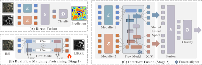
Figure 1: Overview of the proposed FlowErs framework for multimodal land-cover classification. (A) Conventional direct feature fusion, in which modality-specific features extracted from hyperspectral imagery (HSI) and light detection and ranging (LiDAR) data are concatenated directly before classification. (B) Stage 1: Bidirectional multimodal flow-matching pretraining. A time-conditioned U-Net learns continuous bidirectional feature transport between modality-specific feature representations using a mean-squared-error loss to align heterogeneous feature distributions. (C) Stage 2: Interflow fusion. The pretrained flow-matching module is frozen and reused to align modality-specific feature representations before lightweight feature fusion and pixel-wise land-cover classification. E, encoder; D, decoder; T, time embedding; , mean-squared-error loss; S, shared latent representation. Please click here to view a larger version of this figure.

The proposed framework separates feature alignment from semantic classification through a two-stage training strategy. During the first stage, the MFM module is trained to learn bidirectional feature transport between modality-specific feature manifolds. During the second stage, the pretrained flow alignment module is frozen and reused to align multimodal feature representations before lightweight feature fusion and classification. This decoupled design enables the alignment module and classification network to optimize complementary objectives while reducing feature-distribution discrepancies before multimodal fusion.

Theoretical Overview

Flow matching is a recently proposed generative modeling paradigm that learns a continuous deterministic transformation between two probability distributions. Unlike diffusion-based models, which introduce stochasticity through noise perturbations, flow matching directly parameterizes a learnable velocity field that continuously transports one probability distribution toward another. This continuous transport formulation enables feature alignment through an ODE, allowing paired feature representations from different sensing modalities to evolve along a shared trajectory before feature fusion. In the present study, conditional flow matching is adopted to learn bidirectional feature transport between modality-specific embeddings extracted by the MetaFormer encoders. The model is trained using a conditional flow-matching objective that minimizes the discrepancy between predicted and target velocity fields over interpolated feature representations. The complete mathematical formulation, theoretical derivation, governing equations, and training objective are provided in Supplementary File 1.

Problem Formulation

Land-cover classification from multimodal remote sensing data involves learning semantic representations from heterogeneous sensing modalities, such as HSI and LiDAR. These modalities exhibit distinct sensing characteristics. HSI acquires rich spectral information with hundreds of channels (), whereas LiDAR provides fine-grained structural information with comparatively few channels (). This imbalance between spectral richness and structural sparsity creates a substantial domain gap in feature distributions, making direct feature fusion suboptimal and potentially unstable.

Formally, given a pair of multimodal inputs,  the objective is to predict a pixel-wise semantic map according to Equation 1:

Here,  is the one-hot encoded label tensor, C denotes the total number of land-cover categories, and θ represents all learnable model parameters. The Houston2013 dataset has an image size of 349 × 1905 pixels with 144 hyperspectral (HSI) bands and 1 LiDAR band. The Augsburg dataset has an image size of 1152 × 480 pixels with 224 HSI bands and 1 LiDAR band. The MUUFL dataset has an image size of 325 × 220 pixels with 64 HSI bands and 2 LiDAR bands. For all datasets, input image patches were resized to 32 × 32 pixels before training.

Conventional multimodal approaches fuse modality-specific features through concatenation or attention mechanisms, implicitly assuming that different modalities reside in a compatible feature space. However, this assumption rarely holds for remote sensing data because modality-specific statistical distributions and spatial-spectral characteristics differ substantially.

To explicitly bridge this discrepancy, a flow matching module,  is introduced. The module is parameterized by  and learns continuous bidirectional transformations between modality-specific feature manifolds. Specifically (Equation 2),

Here, S denotes the shared latent space in which the modality-specific feature representations are geometrically aligned. Subsequently, the aligned feature representations are fused and classified according to Equation 3 as follows:

Here,  and  denote the feature-fusion and classification modules, respectively. This formulation defines the overall FlowErs framework. Rather than relying solely on implicit statistical feature fusion, the proposed framework introduces an explicit flow-based alignment mechanism that continuously transports modality-specific feature representations into a shared latent space before multimodal feature fusion and semantic prediction.

MetaFormer Encoder

FlowErs performs cross-modal feature alignment using lightweight modality-specific encoders that learn informative and geometrically consistent feature representations from each sensing modality. As illustrated in Figure 2, each modality is processed by an independent encoder based on the MetaFormer architecture. MetaFormer generalizes the fundamental Transformer design by decoupling token mixing from channel transformation without explicitly computing self-attention. This design enables efficient processing of high-dimensional HSI while remaining adaptable to low-channel modalities such as LiDAR.

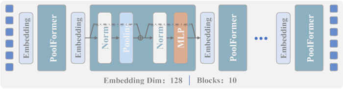
Figure 2: Architecture of the modality-specific MetaFormer encoder used in the proposed FlowErs framework. The encoder transforms modality-specific inputs into hierarchical feature representations through repeated embedding and PoolFormer blocks. Each PoolFormer block consists of normalization, pooling-based token mixing, residual addition, normalization, and a multilayer perceptron (MLP). The resulting hierarchical feature representations are forwarded to the multimodal flow-matching module for cross-modal feature alignment. Norm, normalization; MLP, multilayer perceptron. Please click here to view a larger version of this figure.

For each modality , the MetaFormer encoder , transforms the input  into a hierarchy of latent feature representations (Equation 4):

Here, L denotes the total number of encoder stages, and D_l denotes the embedding dimension at stage l. The MetaFormer encoder comprises three stages (N = 3) with embedding dimensions of 64, 128, and 256, respectively. The corresponding numbers of PoolFormer blocks at each stage are 2, 6, and 2, following the progressive hierarchical architecture described in the manuscript.

Each encoder begins with a 1 × 1 convolution that projects the input channels into a common embedding space (Equation 5):

This projection layer is followed by L stacked MetaFormer blocks. Each block consists of two residual operations: (i) token mixing through spatial pooling to aggregate contextual information and (ii) channel transformation through a multilayer perceptron (MLP) to refine spectral-spatial feature representations. These operations are expressed using Equations 6 and 7 as follows:

Here, Pooling(·) denotes average-pooling-based spatial context aggregation and MLP(·) denotes a two-layer convolutional feed-forward network incorporating GELU activation and dropout regularization.

The encoder follows a hierarchical architecture in which the embedding dimension increases progressively across successive stages (for example, 64 128 256). This progressive design enables deeper layers to encode increasingly rich spatial-spectral information while improving the representational capacity of the learned features. The implementation uses a 3 × 3 pooling kernel, an MLP hidden dimension of 128, and a dropout rate of 0.1. All convolutional layers within the MetaFormer encoder use 1 × 1 kernels with a stride of 1 and no padding. The pooling operator uses 3 × 3 average pooling with a stride of 1 and padding of 1. Batch normalization (BatchNorm2d) is used throughout the encoder. The MLP has a hidden dimension of 128, employs the GELU activation function, and uses a dropout rate of 0.1. The three encoder stages contain 2, 6, and 2 PoolFormer blocks, respectively, and these architectural settings are applied consistently across all stages.

Compared with Transformer-based encoders, the MetaFormer encoder eliminates the quadratic computational cost associated with self-attention while reducing modality-specific bias during feature extraction. Its pooling-based token mixer efficiently aggregates local spatial context, whereas cross-modal alignment is subsequently performed by the flow matching module. Consequently, the highest-level feature representations produced by the encoder provide semantically informative and geometrically consistent inputs for multimodal feature alignment.

Multimodal Flow Matching

The primary challenge following feature extraction is the alignment of heterogeneous feature representations originating from distinct sensing modalities that reside on different feature manifolds. Direct concatenation of  and  often performs poorly because of inconsistent feature distributions and modality-specific biases. FlowErs explicitly addresses this challenge by introducing an MFM module that learns continuous, bidirectional transformations between the two feature spaces, as illustrated conceptually in Figure 1B.

Let  denote the feature representations extracted by the MetaFormer encoders. A continuous flow field parameterized by the interpolation time  is defined using Equation 8 as follows:

Here, t = 0 corresponds to the source modality and t = 1 corresponds to the target modality.

The flow matching model, is implemented as a time-conditioned U-Net that predicts the instantaneous velocity field governing the transformation along this interpolation trajectory. Each flow predictor comprises three downsampling blocks (64  128 256 512) and three corresponding upsampling blocks (512 256 128 64) using 3 × 3 convolutions, batch normalization, and rectified linear unit (ReLU) activation. Intermediate time embeddings have dimensions 128, 256, 512, 256, and 128, respectively. The time embedding uses a fixed sinusoidal positional encoding. ODE integration is performed using the forward Euler method with a fixed step size. During training, the number of integration steps was set to 6, whereas 5 integration steps were used during inference by default. The actual number of integration loop iterations is computed as

The predicted velocity field is given by Equation 9 as follows:

Here,  denotes the predicted instantaneous velocity. The model learns to approximate the displacement   thereby encouraging continuous transformations between modality-specific feature spaces. The training objective is formulated as a time-conditioned bidirectional mean-squared-error (MSE) loss as follows (Equation 10):

 (10)

Sampling t from the specified Beta distribution exposes the model to intermediate interpolation states but does not establish exact cycle consistency. Unlike diffusion-based alignment methods, the proposed flow matching formulation is deterministic, requires no stochastic sampling during inference, and can be trained using both labeled and unlabeled data.

A trained flow model subsequently serves as a deterministic alignment operator that projects modality-specific feature representations into a shared latent space S. The aligned representations are obtained as follows (Equation 11):

Here,  and  denote the aligned feature representations. Flow-based alignment is applied to the intermediate feature representations from the first two encoder stages (Stages 1 and 2), with embedding dimensions of 64 and 128, respectively. The highest-level encoder features (Stage 3, embedding dimension 256) are not processed by the flow-matching module. Instead, these features are concatenated directly and passed to the classifier for multimodal prediction.

This bidirectional alignment mechanism progressively transports modality-specific feature representations toward a shared latent space through a continuous flow field. Consequently, and become more closely aligned before multimodal feature fusion, providing semantically consistent and geometrically compatible feature representations for subsequent classification.

Training Pipeline

FlowErs exploits both labeled and unlabeled data while maintaining stable cross-modal alignment through a two-stage training strategy, as illustrated in Figure 1(B,C). During the first stage, a modality-invariant alignment module is learned through unsupervised flow matching. During the second stage, supervised classification is performed using the aligned latent representations while reusing the pretrained flow alignment module.

Stage 1: Unsupervised Flow Pretraining

Given multimodal image pairs,   modality-specific feature representations,   are extracted using the MetaFormer encoders. Intermediate feature representations are generated using the interpolation defined in Equation 8, where The flow matching module, , is optimized by minimizing the bidirectional time-conditioned objective defined in Equation 10 without using class labels. During this stage, only the flow-matching parameters, , are updated, allowing the model to learn geometry-aware correspondences from both labeled and unlabeled samples before supervised classification. Stage 1 (flow-matching pretraining) was performed using the AdamW optimizer with a learning rate of 1 × 10⁻⁴, a weight decay of 1 × 10⁻², and a cosine annealing learning-rate schedule. Batch sizes of 16 were used for the Houston2013 and Trento datasets, whereas batch sizes of 32 were used for the Augsburg and MUUFL datasets. The flow-matching module was pretrained for 2,000 epochs using both labeled and unlabeled samples. The random seed was fixed at 3407. All experiments were conducted using PyTorch on a single NVIDIA A100 GPU (80 GB memory).

Stage 2: Supervised Classification with a Shared Aligner

The pretrained flow matching module is reused during supervised training and is applied to the first two encoder stages rather than to all feature levels. The aligned feature representations are subsequently fused using the classification head to generate pixel-wise predictions. Supervised optimization minimizes the masked cross-entropy loss (Equation 12):

Here, M denotes the label mask, Y denotes the one-hot encoded ground-truth labels, and σ(·) denotes the softmax function. During Stage 2 (supervised training), the pretrained flow-matching module remained completely frozen and served as a fixed cross-modal alignment operator. Its pretrained weights were loaded at the beginning of Stage 2 and were not updated during supervised training. Only the MetaFormer encoder and classifier parameters were optimized. Supervised training was performed using the AdamW optimizer with dataset-specific learning rates of 1 × 10⁻⁴ (Houston2013), 1 × 10⁻³ (Augsburg), 1 × 10⁻² (MUUFL), and 1 × 10⁻⁵ (Trento). Weight decay was set to 1 × 10⁻² for all datasets except MUUFL, for which a value of 5 × 10⁻² was used. Batch sizes of 16 or 32 were employed depending on the dataset. Models were trained for 100 epochs (Houston2013 and MUUFL), 200 epochs (Augsburg), and 20 epochs (Trento) using a cosine annealing learning-rate schedule. CrossEntropyLoss with mean reduction was used as the loss function. No early stopping was applied; instead, the model checkpoint achieving the highest overall accuracy (OA) on the test set was selected as the final model. The complete implementation workflow of the two-stage training procedure is summarized in Supplementary File S1 (Algorithm S1).

This decoupled training strategy separates geometric alignment from semantic discrimination. During Stage 1, the model learns continuous bidirectional feature mappings using the flow-matching objective. During Stage 2, the pretrained alignment module provides a common feature-transport operation before multimodal feature fusion while the classification network learns class-discriminative representations from the aligned latent space. Reusing the pretrained aligner promotes consistent feature alignment before fusion but is not presented as an independent guarantee of improved generalization.

Experimental Datasets

The proposed framework was evaluated using three representative multimodal remote sensing benchmark datasets: Houston2013²⁹, Augsburg³⁰, and MUUFL³¹.

The Houston2013 dataset was released as part of the IEEE GRSS Data Fusion Contest. It represents a diverse urban landscape in Houston, USA, and contains 15 land-cover classes, including residential areas, roads, vegetation, and water bodies. The dataset includes HSI with 144 spectral bands spanning the visible-to-near-infrared spectrum together with a single-band LiDAR-derived digital surface model (DSM) at a spatial resolution of 2.5 m. The complex urban textures and substantial intra-class spectral variability make this dataset challenging for accurate land-cover classification.

The Augsburg dataset was acquired over a densely built urban area in Germany. It comprises hyperspectral imagery with 224 spectral bands covering the 400–1000 nm wavelength range together with co-registered LiDAR elevation data. The dataset contains 17 annotated land-cover classes, including built structures, bare soil, asphalt, vegetation, and shadow, at a spatial resolution of 2 m. Compared with Houston2013, Augsburg exhibits stronger spectral correlations together with greater class diversity, providing a challenging benchmark for evaluating cross-modal feature alignment and generalization.

The MUUFL Gulfport dataset was collected over a university campus and represents a semi-urban environment containing abundant vegetation together with small man-made structures. The dataset includes denoised 64-band hyperspectral imagery together with dual-band LiDAR measurements consisting of elevation and intensity information. It contains 11 land-cover classes and exhibits fine spatial detail, mixed pixels, and varying illumination conditions, making it well suited for evaluating multimodal feature fusion for small-object classification.

Collectively, these three benchmark datasets encompass substantial variation in spatial resolution (1–2.5 m), spectral dimensionality (64–224 bands), scene complexity, and land-cover composition. Consequently, they provide a diverse benchmark for evaluating the effectiveness and generalizability of multimodal land-cover classification methods. The principal characteristics of the datasets are summarized in Table 1. The train/test partitions for all three datasets correspond to the official benchmark splits provided by the original data providers. Specifically, the Houston2013 dataset uses the official partition from the 2013 IEEE GRSS Data Fusion Contest, comprising 2,832 training samples and 12,197 test samples. The Augsburg dataset uses the officially provided mask_train and mask_test annotations, yielding 4,538 training samples and 47,896 test samples. The MUUFL dataset uses the official train_test_gt.mat partition, containing 28,645 training samples and 24,283 test samples. For each dataset, a 32 × 32-pixel image patch centered on each labeled pixel was extracted as an individual training or test sample. No additional data splitting or resampling was performed.

Property	Houston2013	Augsburg	MUUFL
HSI image size (pixels)	349 × 1905	1152 × 480	325 × 220
LiDAR image size (pixels)	349 × 1905	1152 × 480	325 × 220
HSI spectral bands	144	224	64
LiDAR bands	1	1	2
HSI wavelength range	0.38–1.05 µm	0.40–1.00 µm	375–1050 nm
LiDAR wavelength range	Not applicable	Not applicable	Not applicable
Spatial resolution (HSI)	2.5 m	2.0 m	0.54 m × 1.00 m
Spatial resolution (LiDAR)	2.5 m	2.0 m	0.60 m × 0.78 m
Number of land-cover classes	15	17	11

Table 1: Characteristics of the three multimodal remote sensing benchmark datasets used for evaluation. The table summarizes the image dimensions, spectral characteristics, spatial resolutions, and numbers of land-cover classes for the Houston2013, Augsburg, and MUUFL benchmark datasets used to evaluate the proposed FlowErs framework.

Implementation Details

The FlowErs framework was implemented in PyTorch and trained and evaluated using a graphics processing unit (GPU) with 80 GB of memory. Training was performed for 100 epochs using a batch size of 16. The AdamW optimizer was employed with an initial learning rate of 1 × 10⁻⁴ and a weight decay of 1 × 10⁻². A cosine annealing learning-rate scheduler was used to update the learning rate throughout training. A dropout rate of 0.1 was applied to improve model generalization and reduce overfitting. The cross-entropy loss function was used for supervised optimization. For reproducibility, all experiments were initialized using a fixed random seed of 3407. The supplied train/test partitions were used without creating an additional validation split. Each input patch was resized to 32 × 32 pixels before training. No data augmentation, explicit image-registration correction, or additional data-loader normalization was applied. Pixels associated with negative labels were excluded from the supervised loss calculation. Missing or noisy pixel handling was not evaluated separately.

Evaluation Metrics

Three widely adopted evaluation metrics were used to assess classification performance: OA, Average Accuracy (AA), and the Kappa coefficient (k). OA measures the proportion of correctly classified samples among all samples, AA represents the mean classification accuracy across all land-cover classes, and the Kappa coefficient quantifies the agreement between the predicted and reference classifications after accounting for chance agreement. Higher values of all three metrics indicate better classification performance. All values reported in Tables 2–6 are fixed-split point estimates obtained using the random seed 3407. No confidence intervals, statistical significance tests, or p-values are reported.

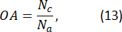
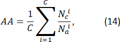
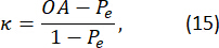
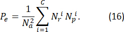
Here, N_c and N_a denote the total numbers of correctly classified samples and evaluated samples, respectively.  and  denote the numbers of correctly classified samples and total samples for the i-th class, respectively. In the calculation of the Kappa coefficient, P_e denotes the probability of agreement occurring by chance, and  and  denote the reference and predicted sample counts for the i-th class, respectively.

Results

The overall evaluation workflow of the proposed FlowErs framework is illustrated in Figure 1, which summarizes the two-stage multimodal classification strategy. The modality-specific feature extraction process based on the MetaFormer encoder is shown in Figure 2, and the principal characteristics of the three benchmark datasets used for evaluation are summarized in Table 1. Classification performance was subsequently evaluated on the MUUFL, Houston2013, and Augsburg benchmark datasets using the OA, AA, and Kappa coefficient (κ) defined in the Protocol section.

Comparison with Other Methods

Several benchmark multimodal classification networks were included to provide a comprehensive comparison of the proposed framework. DFINet³² integrates hyperspectral and multispectral information using a depth-wise cross-attention module to improve feature interaction through multiple loss objectives. DSHFNet³³ introduces a dynamic hierarchical fusion strategy that progressively combines fine-scale and coarse-scale representations. MDL-Middle³⁴ employs an intermediate-layer feature fusion strategy to balance information from multiple sensing modalities. CMCL³⁵ treats HSI and LiDAR data as complementary views of the same scene and applies contrastive learning together with dual fine-tuning to improve feature alignment. Two-Branch³⁶ uses a dual-path convolutional architecture that independently processes each modality before feature fusion. ExViT³⁷ performs multimodal patch processing using parallel Transformer branches with cross-modal attention modules. DSymFuse³⁸ extends the dual-branch Transformer architecture through hierarchical local-global feature fusion. CTPMSN³⁹ combines convolutional and Transformer architectures with text-visual prompt alignment to improve semantic consistency and class discrimination. The comparison values were obtained from the cited publications or their reported evaluation protocols and were not generated using a unified implementation or common experimental framework. Therefore, these comparisons should be interpreted as descriptive benchmark comparisons rather than controlled head-to-head evaluations.

MUUFL dataset

The classification results obtained for the MUUFL Gulfport dataset are summarized in Table 2, and representative classification maps are presented in Figure 3A–J. On the reported fixed benchmark split, the proposed framework achieved an OA of 95.24% and a Kappa coefficient of 93.69%, compared with 93.99% and 92.03%, respectively, for CTPMSN. Class-level performance varied across land-cover categories. Compared with CTPMSN, the proposed framework achieved higher classification accuracies for the Trees, Mostly Grass, and Mixed Surface classes by 2.73%, 3.16%, and 1.86%, respectively. In contrast, the Yellow Curb class remained challenging because of the limited number of available samples, and its reported accuracy was lower than that of several comparison methods. Accordingly, the observed improvement in aggregate performance should not be interpreted as indicating superior performance for every individual land-cover class. The qualitative comparison in Figure 3A–I shows the classification maps generated by the evaluated methods, whereas Figure 3J presents the corresponding ground-truth reference map, illustrating the spatial distribution of the land-cover classes across the MUUFL Gulfport dataset.

Class	DFINet	DSHFNet	MDL-Middle	CMCL	Two-Branch	ExVit	DSymFuse	CTPMSN	FlowErs
Trees	89.2	74.91	87.31	84.86	91.32	92.64	91.24	95.55	98.28
Mostly grass	72.98	84.63	76.38	86.54	80.65	77.48	79.57	88.92	92.08
Mixed surface	69.22	34.77	68.33	54.75	67.92	82.07	82.23	87.92	89.78
Dirt/sand	76.68	87.06	78.74	84.45	78.32	93.74	89.17	97.27	93.55
Road	86.68	81.09	83.76	86.25	84.34	90.35	85.6	94.52	95.94
Water	100	99.25	88.52	98.53	100	99.38	100	100	97.56
Shadow	83.29	90.65	92.12	97.72	84.89	91.47	91	95.98	90.54
Building	93.26	90.22	89.69	97.54	93.76	89.27	96.29	96.29	98.26
Sidewalk	57.34	53.09	77.06	77.98	71.32	73.54	79.62	88.07	79.61
Yellow curb	84.28	1.03	96.75	80.62	81.41	93.72	91.57	97.37	48.91
Cloth panels	97.92	92.79	99.41	98.41	99.21	99.41	100	99.41	93.13
Overall accuracy (OA)	83.87	74.29	83.54	82.45	85.61	89.94	88.78	93.99	95.24
Average accuracy (AA)	82.76	73.23	84.37	85.9	85.1	90.12	89.54	94.68	88.88
Kappa coefficient (κ × 100)	79.82	67.92	78.84	78.37	81.22	85.37	85.37	92.03	93.69

Table 2: Classification performance (%) of different methods on the MUUFL benchmark dataset. Per-class classification performance together with the overall accuracy (OA), average accuracy (AA), and Kappa coefficient (κ) obtained by the proposed FlowErs framework and competing methods on the MUUFL benchmark dataset.

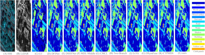
Figure 3: Representative land-cover classification results for the MUUFL benchmark dataset. (A) Hyperspectral imagery (HSI). (B) Light detection and ranging (LiDAR) image. (C) Ground-truth (GT) reference map. (D–L) Classification maps generated by DFINet, DSHFNet, MDL-Middle, CMCL, Two-Branch, ExVit, DSymFuse, CTPMSN, and the proposed FlowErs framework, respectively. The color legend identifies the land-cover classes represented in each classification map.Please click here to view a larger version of this figure.

Houston2013 dataset

The classification results obtained for the Houston2013 dataset are presented in Table 3, and representative classification maps are shown in Figure 4A–J. On the reported fixed benchmark split, the proposed framework achieved an OA of 97.56% and a Kappa coefficient of 97.39%. Compared with the reported CTPMSN results, the proposed framework demonstrated an approximately 3.8 percentage point higher OA. Improvements were also observed for the Residential and Highway classes, with reported increases of approximately 2.4 and 0.5 percentage points, respectively. However, the Commercial class remained comparatively challenging and exhibited lower classification accuracy than several competing methods, which may reflect spectral and spatial similarity with other urban land-cover categories. Overall, the aggregate results indicate improved classification performance on this benchmark while demonstrating that performance varied across individual classes. The qualitative comparison in Figure 4A–I shows the classification maps generated by the evaluated methods, whereas Figure 4J presents the corresponding ground-truth reference map, illustrating the spatial distribution of the land-cover classes across the Houston2013 dataset.

Class	DFINet	DSHFNet	MDL-Middle	CMCL	Two-Branch	ExVit	DSymFuse	CTPMSN	FlowErs
Healthy grass	82.39	85.58	83.1	82.91	80.31	81.67	80.06	96.96	100
Stressed grass	100	94.65	85.06	95.68	92.44	100	78.67	94.27	96.94
Synthetic grass	100	98.12	99.6	94.93	99.23	99.01	99.41	99.41	99.84
Tree	100	93.09	91.57	93.37	98.75	98.96	95.55	96.21	99.6
Soil	98.76	99.91	98.86	99.43	99.2	99.91	98.67	99.43	100
Water	94.5	93.1	100	97.3	95.32	100	95.8	100	97.6
Residential	87.5	66.65	97.64	92.58	90.87	93.28	87.22	86.86	99.29
Commercial	91.53	76.29	88.13	87.96	95.31	89.27	85.85	94.61	84.07
Road	84.19	36.29	85.93	80.76	82.63	89.42	93.29	88.07	92.73
Highway	69.32	89	74.42	57.41	66.69	71.33	67.95	81.66	99.74
Railway	96.76	94.78	84.54	79.57	93.44	92.88	79.13	97.7	99.72
Parking Lot 1	83.27	88.39	95.39	52.83	85.67	89.63	91.07	93.28	95.42
Parking Lot 2	85.36	96.46	87.37	92.42	86.17	89.47	84.21	95.09	99.18
Tennis Court	100	97.3	95.14	83.04	98.72	97.89	100	100	99.72
Running Track	99.21	100	100	97.02	100	97.97	100	100	99.83
Overall accuracy (OA)	91.21	85.02	89.55	83.87	90.01	91.57	87.57	93.74	97.56
Average accuracy (AA)	92.42	87.55	91.05	85.76	90.98	92.32	89.09	94.9	97.58
Kappa coefficient (κ × 100)	91.09	83.59	87.59	82.76	89.1	90.85	85.29	93.21	97.39

Table 3: Classification performance (%) of different methods on the Houston2013 benchmark dataset. Per-class classification performance together with the overall accuracy (OA), average accuracy (AA), and Kappa coefficient (κ) obtained by the proposed FlowErs framework and competing methods on the Houston2013 benchmark dataset.

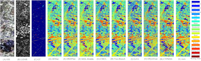
Figure 4: Representative land-cover classification results for the Houston2013 benchmark dataset. (A) Hyperspectral imagery (HSI). (B) Light detection and ranging (LiDAR) image. (C) Ground-truth (GT) reference map. (D–L) Classification maps generated by DFINet, DSHFNet, MDL-Middle, CMCL, Two-Branch, ExVit, DSymFuse, CTPMSN, and the proposed FlowErs framework, respectively. The color legend identifies the land-cover classes represented in each classification map. Please click here to view a larger version of this figure.

Augsburg dataset

The classification results obtained for the Augsburg dataset are summarized in Table 4, and representative classification maps are presented in Figure 5A–J. This dataset is characterized by substantial intra-class variation and complex background structure. On the reported fixed benchmark split, the proposed framework achieved an OA of 97.56% and an AA of 89.21%. Compared with the listed benchmark methods, the proposed framework reported higher classification accuracies for the Industrial and Commercial classes by approximately 14 and 45 percentage points, respectively. The difference between OA and AA indicates that overall performance was influenced by class frequency, whereas AA reflects the average performance across all classes. Accordingly, the reported OA should be interpreted together with the class-wise results because classification performance varied among individual land-cover categories. The qualitative comparison in Figure 5A–I shows the classification maps produced by the evaluated methods, whereas Figure 5J presents the corresponding ground-truth reference map, illustrating the spatial distribution of the land-cover classes across the Augsburg dataset.

Class	DFINet	DSHFNet	MDL-Middle	CMCL	Two-Branch	ExVit	DSymFuse	CTPMSN	FlowErs
Trees	96.41	98.21	91.72	94.27	95.85	93.64	90.58	93.36	99.57
Residential	96.88	42.08	95.19	69.84	92.75	97.71	96.32	97.37	98.97
Industrial	58.2	47.29	62.61	35.22	72.66	65.82	72.45	64.6	86.41
Low plants	92.22	51.75	87.76	80.27	88.9	84.88	89.65	96.72	99.58
Allotment	55.87	95.94	50.86	89.33	72.86	46.85	62.91	58.69	91.22
Commercial	10.98	50.91	24.24	45.59	20.32	24.49	17.22	29.73	74.3
Water	22.87	67.78	29.04	54.87	36.82	24.49	13.27	15.53	74.39
Overall accuracy (OA)	88.78	56.59	87.74	75.94	87.29	87.72	88.35	91.56	97.56
Average accuracy (AA)	62.29	65.47	63.06	67.61	67.78	62.56	63.2	65.14	89.21
Kappa coefficient (κ × 100)	84.32	46.78	82.69	67.83	82.58	82.49	83.36	87.88	96.48

Table 4: Classification performance (%) of different methods on the Augsburg benchmark dataset. Per-class classification performance together with the overall accuracy (OA), average accuracy (AA), and Kappa coefficient (κ) obtained by the proposed FlowErs framework and competing methods on the Augsburg benchmark dataset.

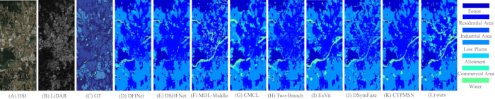
Figure 5: Representative land-cover classification results for the Augsburg benchmark dataset. (A) Hyperspectral imagery (HSI). (B) Light detection and ranging (LiDAR) image. (C) Ground-truth (GT) reference map. (D–L) Classification maps generated by DFINet, DSHFNet, MDL-Middle, CMCL, Two-Branch, ExVit, DSymFuse, CTPMSN, and the proposed FlowErs framework, respectively. The color legend identifies the land-cover classes represented in each classification map. Please click here to view a larger version of this figure.

To facilitate closer visual comparison of challenging regions, enlarged views of representative ROIs from the MUUFL, Houston2013, and Augsburg datasets are presented in Figure 6. These enlarged views highlight object boundaries and fine-scale spatial structures that are less apparent in the full-scene classification maps shown in Figures 3–5, providing additional qualitative evidence of the classification performance across the three benchmark datasets.

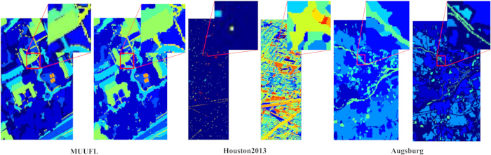
Figure 6: Enlarged views of representative regions of interest (ROIs) from the MUUFL, Houston2013, and Augsburg datasets. Representative ROIs from the MUUFL, Houston2013, and Augsburg datasets are enlarged to facilitate visual comparison of fine-scale classification details. Red boxes indicate the selected regions, and the corresponding enlarged views highlight object boundaries, small structures, and other challenging areas that are difficult to appreciate in the full-scene classification maps shown in Figures 3–5. These enlarged views provide additional qualitative assessment of the classification results. Please click here to view a larger version of this figure.

Ablation Study

Effect of the multimodal flow matching module:

To evaluate the contribution of the MFM module, ablation experiments were performed using three model configurations: the complete FlowErs framework (Baseline), a model without the MFM module (w/o MFM), and a simplified model employing unidirectional flow alignment (Single Flow). The corresponding quantitative results are summarized in Table 5.

Method	MUUFL			Houston2013			Augsburg
	OA (%)	AA (%)	κ × 100	OA (%)	AA (%)	κ × 100	OA (%)	AA (%)	κ × 100
Baseline	95.24	88.88	93.69	97.56	97.58	97.39	97.56	89.21	96.48
w/o MFM	92.87	86.02	91.05	95.31	95.28	94.97	95.12	87.06	93.98
Single Flow	94.38	87.43	92.72	96.58	96.47	96.22	96.47	88.36	95.47

Table 5: Ablation study of the proposed FlowErs framework on the MUUFL, Houston2013, and Augsburg benchmark datasets. Classification performance is reported for the complete model (Baseline) and two ablation variants using overall accuracy (OA), average accuracy (AA), and the Kappa coefficient (κ).

Compared with the Baseline model, removal of the MFM module resulted in lower OA, AA, and Kappa values across all three benchmark datasets. The Single Flow configuration produced intermediate performance between the complete model and the model without MFM, indicating that unidirectional feature alignment retained part of the observed performance improvement while not reaching the aggregate performance of the bidirectional implementation. These observations suggest that the bidirectional flow alignment module contributed to the reported performance under the evaluated benchmark settings. The reported differences represent fixed-split point estimates obtained using a single random seed and should therefore be interpreted descriptively rather than as evidence of statistical significance.

Across the three benchmark datasets, the largest aggregate performance differences between the Baseline and ablation models were observed on the MUUFL dataset, whereas comparatively smaller differences were observed on the Houston2013 dataset. Improvements in both OA and AA were observed for the complete model relative to the ablation configurations, indicating higher aggregate classification performance together with improved average class performance under the evaluated benchmark splits. These findings are consistent with the study hypothesis that feature alignment before multimodal fusion may improve classification performance; however, repeated experiments and statistical analyses were not performed in the present study.

Effect of the Number of Flow Integration Steps:

To further evaluate the influence of the number of flow integration steps within the MFM module, the number of integration steps was varied from 2 to 10. The corresponding classification results are summarized in Table 6. The integration step parameter controls the discretization of the continuous feature-transport process during multimodal alignment, with smaller values representing coarser discretization and larger values representing finer discretization. As shown in Table 6, the highest fixed-split point estimates across the evaluated metrics were obtained when the number of integration steps was 6. Performance generally improved as the number of integration steps increased from 2 to 6, after which the reported performance remained relatively stable or decreased slightly across the three benchmark datasets. These observations indicate that the nominal setting of six integration steps provided the highest aggregate performance under the evaluated benchmark conditions. Because the reported results are based on a single random seed and fixed benchmark splits, these differences should be interpreted descriptively rather than as evidence of statistically significant performance differences.

Flow integration steps	MUUFL			Houston2013			Augsburg
	OA (%)	AA (%)	κ × 100	OA (%)	AA (%)	κ × 100	OA (%)	AA (%)	κ × 100
2	92.37	84.63	90.12	95.73	96.12	95.64	94.86	85.73	92.76
3	93.58	85.47	90.98	96.32	96.48	96.01	95.61	86.48	93.51
4	94.31	86.51	91.76	96.88	96.92	96.57	96.18	87.34	94.12
5	94.92	87.62	92.54	97.18	97.22	97.05	96.89	88.02	95.07
6	95.24	88.88	93.69	97.56	97.58	97.39	97.56	89.21	96.48
7	95.12	88.56	93.5	97.49	97.44	97.31	97.34	88.84	96.21
8	94.95	88.22	93.2	97.31	97.29	97.17	96.98	88.46	95.82
9	94.63	87.75	92.85	97.09	97.03	96.88	96.45	87.92	95.28
10	94.21	86.97	92.18	96.77	96.81	96.61	95.87	87.03	94.61

Table 6: Effect of the number of flow integration steps on classification performance for the MUUFL, Houston2013, and Augsburg benchmark datasets. Classification performance is reported as overall accuracy (OA), average accuracy (AA), and the Kappa coefficient (κ) for different numbers of flow integration steps. Six integration steps correspond to the configuration used in the final FlowErs framework.

Among the evaluated datasets, the MUUFL dataset exhibited the largest variation in performance as the number of integration steps changed, whereas the Houston2013 dataset showed comparatively smaller changes while also achieving its highest reported performance at six integration steps. The Augsburg dataset demonstrated a similar trend with relatively modest performance variation across different step settings. Collectively, these observations suggest that a moderate number of flow integration steps provided the highest reported classification performance for the evaluated datasets. The present analysis does not include repeated experiments, uncertainty estimates, computational profiling, robustness to missing modalities or noisy inputs, or cross-region generalization, and therefore no conclusions are drawn regarding these aspects.

The evaluation across the three benchmark datasets demonstrated competitive aggregate classification performance under the reported fixed benchmark splits, with a maximum OA of 97.56%. The ablation experiments showed that the complete bidirectional flow-matching configuration consistently achieved higher aggregate performance than the corresponding ablation models across the evaluated datasets. Class-wise analyses indicated that classification performance varied among land-cover categories, with minority classes and spectrally similar categories remaining comparatively challenging and contributing to the observed difference between OA and AA on imbalanced datasets. The present evaluation is based on fixed-split point estimates obtained using a single random seed and does not include repeated-run uncertainty estimates, statistical significance testing, computational profiling, sensitivity to spatial misregistration, robustness to missing or noisy modalities, or cross-region generalization. These aspects warrant further investigation in future studies.

Data Availability:

The public benchmark datasets used in this study are available from their original providers. The implementation materials, prediction maps, and evaluation outputs are publicly available through the Zenodo repository at https://doi.org/10.5281/zenodo.21395701.

Supplementary File 1: Mathematical formulation and training algorithm of the FlowErs framework. This supplementary file provides the complete mathematical formulation underlying the proposed FlowErs framework, including the continuous flow formulation (Equations S1–S2), probability flow equation (Equation S3), optimal flow path (Equations S4–S5), conditional flow-matching training objective (Equation S6), and the associated theoretical properties. The file also includes Algorithm S1, which summarizes the complete two-stage training workflow comprising unsupervised flow-matching pretraining followed by supervised multimodal classification.

Discussion

The present study introduces FlowErs, a multimodal remote sensing framework that separates cross-modal feature alignment from semantic classification through a two-stage learning strategy. Rather than directly fusing heterogeneous modality-specific features, the proposed framework first aligns feature representations using conditional flow matching before multimodal fusion and classification. This design addresses the long-standing challenge of heterogeneous feature distributions between HSI and LiDAR, where differences in sensing mechanisms often limit the effectiveness of conventional concatenation- or attention-based fusion strategies^{23,26,35,36,37,38,39}. By formulating multimodal alignment as continuous feature transport, FlowErs extends recent developments in flow matching from generative modeling toward multimodal remote sensing representation learning^{15,16,17,18,19,20,21}. Under the evaluated benchmark conditions, the proposed framework achieved competitive aggregate classification performance on the Houston2013, Augsburg, and MUUFL datasets, while the accompanying ablation study further supported the contribution of the bidirectional flow alignment module to the reported fixed-split performance.

The reported findings suggest that explicit feature alignment before multimodal fusion may improve the compatibility of heterogeneous feature representations extracted from different sensing modalities. Previous multimodal remote sensing methods have primarily relied on convolutional networks, Transformer-based architectures, attention mechanisms, contrastive learning, or prompt-guided fusion to strengthen feature interaction^{23,26,35,36,37,38,39}. Although these approaches have demonstrated strong classification performance, most assume that modality-specific embeddings can be directly fused after feature extraction. In contrast, FlowErs introduces an intermediate geometric alignment stage that continuously transports modality-specific features into a shared latent space before classification. The class-wise evaluation demonstrates that aggregate performance improvements were not uniformly distributed across all land-cover categories. For example, several minority classes and spectrally similar urban categories remained comparatively difficult to classify, and the observed difference between OA and AA, particularly for the Augsburg dataset, reflects the influence of class imbalance together with variable class-level performance. Accordingly, the reported aggregate metrics should be interpreted alongside the class-wise results rather than as evidence of uniform improvements across every category.

The ablation experiments further support the proposed design. Removing the multimodal flow matching module reduced aggregate classification performance across all three benchmark datasets, whereas the single-direction flow variant consistently performed between the complete model and the model without flow alignment. These observations are consistent with the working hypothesis that bidirectional feature transport may improve cross-modal correspondence before feature fusion under the evaluated benchmark conditions. Similarly, the flow integration analysis demonstrated that intermediate discretization of the learned transport trajectory produced the highest aggregate performance, with six integration steps representing the nominal operating point in the present implementation. Performance gains became marginal or slightly decreased with additional integration steps, suggesting that increasingly fine discretization may provide diminishing returns under the evaluated experimental conditions. Whether this operating point generalizes to other datasets, sensing modalities, or network architectures remains to be investigated.

Several limitations should be considered when interpreting the present findings. First, the evaluation was limited to three publicly available benchmark datasets using fixed train/test partitions and a single random seed. Consequently, repeated-run uncertainty, confidence intervals, statistical significance testing, and inter-run variability were not evaluated. Second, the comparison methods were taken from their respective publications rather than being reimplemented within a common experimental framework; therefore, the reported comparisons should be interpreted descriptively rather than as controlled head-to-head reproductions. Third, robustness to missing modalities, noisy observations, spatial misregistration, and cross-region generalization was not investigated. In addition, although flow matching provides a theoretical framework for continuous and potentially invertible feature transport^15,16,17, exact invertibility, topology preservation, and physical interpretability of the learned transformations were not empirically verified in the present study. Computational characteristics, including inference time, memory consumption, and floating-point operation complexity, were likewise not separately profiled.

Alternative approaches for studying multimodal alignment continue to evolve. Recent studies have explored contrastive learning, graph-based fusion, low-rank representation learning, prompt-guided multimodal learning, federated learning, and hybrid convolutional–Transformer architectures to improve multimodal feature integration^{23,26,27,28,35,36,37,38,39}. These strategies remain complementary rather than mutually exclusive, and future work may investigate combinations of explicit flow-based feature transport with these existing alignment paradigms. Beyond land-cover classification, continuous feature alignment may also be applicable to related multimodal remote sensing tasks, including semantic segmentation, change detection, object recognition, environmental monitoring, disaster assessment, precision agriculture, and urban mapping, where complementary sensing modalities are increasingly available^{2,3,4,5,6,7,8,9,23}.

Future investigations should evaluate the proposed framework under more diverse experimental conditions by incorporating repeated-run statistical analyses, computational profiling, robustness to missing or noisy modalities, sensitivity to spatial registration errors, and cross-region transfer evaluation. Additional studies examining alternative flow parameterizations, different encoder architectures, and larger multimodal benchmark datasets would further clarify the generalizability and practical applicability of the proposed methodology. Collectively, the present results indicate that explicit feature alignment through conditional flow matching represents a promising complementary strategy for multimodal remote sensing classification while highlighting several opportunities for further methodological development and comprehensive evaluation.

Materials

List of materials used in this article

Name	Company	Catalog Number	Comments
AdamW optimizer	PyTorch Foundation	Included in PyTorch	Used for model optimization. PyTorch 2.5.0 was used.
Augsburg benchmark dataset	Hu J et al. (Earth System Science Data, 2022); Remote Sensing Technology, LMU Munich	https://doi.org/10.5281/zenodo.7185498	Public multimodal remote sensing benchmark dataset used for model evaluation.
CUDA Toolkit	NVIDIA	CUDA Toolkit 12.4; https://developer.nvidia.com/cuda-12-4-0-download-archive	Used for GPU-accelerated model training and inference.
Graphics processing unit (GPU)	NVIDIA Corporation	NVIDIA A100 80 GB PCIe	Used for model training and evaluation.
Houston2013 benchmark dataset	IEEE Geoscience and Remote Sensing Society Data Fusion Contest	http://www.grss-ieee.org/community/technical-resources/data-fusion/2013-grss-data-fusion-contest/	Public hyperspectral imagery and LiDAR benchmark dataset used for model evaluation.
MUUFL Gulfport benchmark dataset	University of Florida (Gader P et al., Technical Report REP-2013-570)	https://github.com/GatorSense/MUUFLGulfport	Public hyperspectral imagery and LiDAR benchmark dataset used for model evaluation.
Operating system	Canonical Ltd.	Ubuntu 22.04 LTS; https://ubuntu.com	Computational environment used for model development, training, and evaluation.
PyTorch	PyTorch Foundation	PyTorch 2.5.0; https://pytorch.org/get-started/previous-versions/#v250	Deep learning framework used to implement, train, and evaluate the FlowErs model.
Python	Python Software Foundation	Python 3.11; https://www.python.org/downloads/release/python-3110/	Programming language used to implement and execute the computational workflow.

References

- Geng X, et al. Fast and effective: Progressive hierarchical fusion classification for remote sensing images. IEEE Trans Multimed. 2024;26:9776–89.
- Tian F, et al. HireNet: Hierarchical-relation network for few-shot remote sensing image scene classification. IEEE Trans Geosci Remote Sens. 2024;62:1–10.
- Ye Z, et al. A multiscale incremental learning network for remote sensing scene classification. IEEE Trans Geosci Remote Sens. 2024;62:1–15.
- Li Q, Chen Y, He X, Huang L. Co-training transformer for remote sensing image classification, segmentation, and detection. IEEE Trans Geosci Remote Sens. 2024;62:1–18.
- Qin A, et al. Deep updated subspace networks for few-shot remote sensing scene classification. IEEE Trans Geosci Remote Sens. 2024;62:1–14.
- Wang S, et al. Personalized multiparty few-shot learning for remote sensing scene classification. IEEE Trans Geosci Remote Sens. 2024;62:1–15.
- Yang JY, et al. Multifrequency graph convolutional network with cross-modality mutual enhancement for multisource remote sensing data classification. IEEE Trans Geosci Remote Sens. 2024;62:1–14.
- Zhou G, Qian L, Gamba P. A novel iterative self-organizing pixel matrix entanglement classifier for remote sensing imagery. IEEE Trans Geosci Remote Sens. 2024;62:1–21.
- Zhu J, et al. MVP: Meta visual prompt tuning for few-shot remote sensing image scene classification. IEEE Trans Geosci Remote Sens. 2024;62:1–13.
- Gat I, et al. Discrete flow matching. Adv Neural Inf Process Syst. 2024;37:133345–85.
- Miller BK, Chen RT, Sriram A, Wood BM. FlowMM: Generating materials with Riemannian flow matching [Internet]. 2024 [cited 2026 Jul 6]. Available from: https://arxiv.org/abs/2406.04713
- Xin Y, et al. Confidence-weighted dual-teacher networks with biased contrastive learning for semi-supervised semantic segmentation in remote sensing images. IEEE Trans Geosci Remote Sens. 2024;62:1–16.
- He Y, et al. IGroupSS-Mamba: Interval group spatial-spectral Mamba for hyperspectral image classification. IEEE Trans Geosci Remote Sens. 2024;62:1–14.
- Liao D, Wang Q, Lai T, Huang H. Joint classification of hyperspectral and LiDAR data based on Mamba. IEEE Trans Geosci Remote Sens. 2026;19:11445–61.
- Lipman Y, et al. Flow matching for generative modeling [conference paper]. Presented at: 11th International Conference on Learning Representations (ICLR); 2023. Available from: https://openreview.net/forum id=PqvMRDCJT9t
- Liu X, et al. Flow straight and fast: Learning to generate and transfer data with rectified flow [conference paper]. Presented at: 11th International Conference on Learning Representations (ICLR); 2023. Available from: https://openreview.net/forum id=XVjTT1nw5z
- Geng Z, et al. Consistency models made easy [conference paper]. Presented at: 13th International Conference on Learning Representations (ICLR); 2025. Available from: https://openreview.net/forum id=1x7sJYh37d
- Hu VT, et al. Latent space editing in transformer-based flow matching [conference paper]. Presented at: AAAI Conference on Artificial Intelligence; 2024;38:2247–55. Available from: https://doi.org/10.1609/aaai.v38i3.28014
- Jeong J, Kim K, Kim W, Kim NJ. Real-time person image synthesis using a flow matching model [Internet]. 2025 [cited 2026 Jul 6]. Available from: https://arxiv.org/abs/2505.03562
- Kakesh MH, et al. An efficient data generation method based on flow matching for bearing fault diagnosis under imbalanced data conditions. IEEE Trans Energy Convers. 2026;1–11.
- Chu Z, et al. End-to-end seam tracking with flow matching-based diffusion policy [conference paper]. Presented at: International Conference on Machine Intelligence and Nature-Inspired Computing (MIND); Xiamen, China; 2025. p. 304–9. Available from: https://doi.org/10.1109/MIND67540.2025.11351867
- Melgani F, Bruzzone L. Classification of hyperspectral remote sensing images with support vector machines. IEEE Trans Geosci Remote Sens. 2004;42:1778–90.
- Li J, et al. Deep learning in multimodal remote sensing data fusion: A comprehensive review. Int J Appl Earth Obs Geoinf. 2022;112:102926.
- Vaswani A, et al. Attention is all you need [Internet]. 2017 [cited 2026 Jul 6]. Available from: https://arxiv.org/abs/1706.03762
- Zhuang Y, Chen M, Zhu D. UWASR-GAN: An attention-guided multi-scale residual framework for underwater image enhancement in underwater Internet of Things applications. IEEE Internet Things J. 2026;12:29452–71.
- Ma X, Zhang X, Pun MO, Liu M. A multilevel multimodal fusion transformer for remote sensing semantic segmentation. IEEE Trans Geosci Remote Sens. 2024;62:1–15.
- Xie W, Lu Y, Li D, Li Y. Ebbinghaus-curve guided low-rank component-induced attention for multisource remote sensing classification. IEEE Trans Geosci Remote Sens. 2024;62:1–12.
- Li D, Xie W, Li Y, Fang L. FedFusion: Manifold-driven federated learning for multi-satellite and multi-modality fusion. IEEE Trans Geosci Remote Sens. 2023;62:1–13.
- Debes C, et al. Hyperspectral and LiDAR data fusion: Outcome of the 2013 GRSS data fusion contest. IEEE J Sel Top Appl Earth Obs Remote Sens. 2014;7:2405–18.
- Hu J, et al. MDAS: A new multimodal benchmark dataset for remote sensing. Earth Syst Sci Data Discuss. 2022:1–26.
- Gader P, et al. MUUFL Gulfport hyperspectral and LiDAR airborne data set. University of Florida; Gainesville (FL); Technical Report REP-2013-570; 2013.
- Gao Y, et al. Hyperspectral and multispectral classification for coastal wetland using depthwise feature interaction network. IEEE Trans Geosci Remote Sens. 2021;60:1–15.
- Feng Y, Song L, Wang L, Wang X. DSHFNet: Dynamic scale hierarchical fusion network based on multiattention for hyperspectral image and LiDAR data classification. IEEE Trans Geosci Remote Sens. 2023;61:1–14.
- Hong D, et al. More diverse means better: Multimodal deep learning meets remote-sensing imagery classification. IEEE Trans Geosci Remote Sens. 2020;59:4340–54.
- Feng Z, et al. Cross-modal contrastive learning for remote sensing image classification. IEEE Trans Geosci Remote Sens. 2023;61:1–13.
- Xu X, et al. Multisource remote sensing data classification based on convolutional neural network. IEEE Trans Geosci Remote Sens. 2017;56:937–49.
- Yao J, et al. Extended vision transformer (ExViT) for land use and land cover classification: A multimodal deep learning framework. IEEE Trans Geosci Remote Sens. 2023;61:1–15.
- Chang H, et al. Deep symmetric fusion transformer for multimodal remote sensing data classification. IEEE Trans Geosci Remote Sens. 2024;63:1–15.
- Wang A, et al. CTPMSN: Enhancing multimodal remote sensing classification with composite text prompts. IEEE J Sel Top Appl Earth Obs Remote Sens. 2025;18:27960–27978.