Cross-Site Physics-Informed Transfer Learning for One-Hour-Ahead Photovoltaic Power Forecasting

Summary

This article presents a cross-site physics-informed transfer learning framework for one-hour-ahead photovoltaic power forecasting that combines transfer learning, plant-level descriptors, and physics-informed constraints across heterogeneous solar plants.

Abstract

Accurate short-term photovoltaic power forecasting is essential for grid scheduling, reserve allocation, and the reliable integration of renewable energy into power systems. However, many data-driven forecasting models are trained and evaluated at a single photovoltaic plant, which limits their transferability to plants operating under different climatic, geographic, and engineering conditions. This study evaluated a cross-site physics-informed transfer-learning framework for one-hour-ahead photovoltaic power forecasting across six heterogeneous solar plants. The framework integrated a hybrid temporal model with plant-level static descriptors and a physics-based power prior derived from irradiance, module temperature, installed capacity, and grid export limits. The primary experiment used six leave-one-site-out target folds: for each held-out target plant, the other five plants were pooled as the source domain for pretraining. A separate, ordered single-source-to-single-target analysis (30 routes) was used solely to examine pairwise source-target distances and route-dependent transfer behavior. Source-domain and target-domain validation data were kept separate during checkpoint selection. Compared with direct transfer and conventional fine-tuning in the primary held-out-target analysis, the full physics-informed transfer model reduced forecasting error across the evaluated target sites. The study provides a structured framework for cross-site photovoltaic forecasting under heterogeneous environmental and operational conditions. Because inferential comparisons were based on six held-out target sites, they were interpreted as site-level evidence rather than evidence of broad population-level statistical generalizability.

Introduction

Photovoltaic power generation has become an increasingly important component of modern renewable energy systems, but its variable output continues to pose operational challenges for grid scheduling, reserve planning, and plant-level dispatch. Reliable short-term forecasting is therefore required not only to estimate future generation but also to support the safe coordination of photovoltaic plants with existing grid infrastructure¹. Recent deep-learning methods have improved photovoltaic forecasting accuracy, particularly when sufficient historical data are available for a single plant. Their practical value, however, is often reduced when the same model is deployed at another plant with different weather patterns, topographic conditions, installed capacity, module configuration, inverter type, tracking system, or grid export constraint².

This limitation is especially relevant for newly commissioned or data-scarce photovoltaic plants. In these settings, local historical data may be insufficient to train a stable forecasting model from scratch. Transfer learning offers a practical solution by allowing knowledge learned from data-rich source plants to be adapted to a target plant with limited data³. Yet direct transfer is rarely sufficient in photovoltaic forecasting because the irradiance-to-power relationship is not purely statistical. It is shaped by physical constraints, including solar irradiance, panel temperature, installed capacity, DC/AC ratio, curtailment status, and plant-specific export limits. A transfer model that ignores these operating boundaries may learn patterns that perform well at the source site but fail under the physical and operational conditions of the target site⁴.

Cross-site photovoltaic forecasting, therefore, requires more than the reuse of temporal patterns learned from another plant. Prior multi-site studies suggest that shared learning can improve prediction accuracy, but the benefit depends strongly on the similarity between source and target domains, including climatic regime, seasonal irradiance profile, geographical location, and plant configuration^5,6. When these differences are not explicitly represented, the model may transfer site-specific noise rather than generalizable forecasting knowledge. This is one reason why cross-site generalization remains difficult even when advanced recurrent or convolutional architectures are used.

Physics-informed learning provides a way to reduce this limitation by embedding plant-recognizable physical structure into the forecasting process. Instead of relying solely on measured time-series inputs, a physics-informed model can incorporate a power prior derived from irradiance, temperature, installed capacity, and operational limits^7,8. This prior does not replace data-driven learning, but it constrains the model toward physically plausible behavior when target-site data are scarce or when the distribution differs from that at the source site^8,9. In photovoltaic forecasting, this approach is particularly useful because short-term output is governed by both temporal weather variations and plant-specific engineering constraints¹⁰.

Recent literature has increasingly addressed data scarcity, cross-domain adaptation, and hybrid modeling in photovoltaic forecasting. Bellagarda et al. showed that transfer learning can adapt neural models pretrained on synthetic photovoltaic data to limited real observations^{11,12,13,14,15}, while Miraftabzadeh et al. demonstrated transfer of deep neural representations for photovoltaic prediction under restricted target-domain data¹⁶. More recent work has combined cross-plant transfer with explicit physical knowledge and domain adaptation for newly built photovoltaic plants¹⁷, and hybrid dilated-convolution/recurrent architectures with transfer strategies continue to improve short-term forecasting¹⁸. In parallel, general time-series foundation models such as TimesFM and MOMENT have demonstrated zero- or few-shot transfer across heterogeneous forecasting datasets^19,20, suggesting a broader direction for renewable-energy forecasting when local supervision is limited. Physics-informed hybrid forecasting has also continued to evolve, including multi-site models that combine machine-learning and recurrent components with physical features and uncertainty quantification²¹. These developments motivate a cross-site framework that remains lightweight, physically constrained, and explicitly testable under limited target-site data.

This study evaluated a reproducible framework for cross-site physics-informed transfer learning in one-hour-ahead photovoltaic power forecasting. The framework combined a hybrid temporal neural architecture, plant-level static descriptors, and a physics-based power prior. The primary evaluation followed a sixfold leave-one-site-out design, in which one plant was held out as the target, and the remaining five plants were pooled as the source domain for pretraining. To examine route dependence separately, an additional pairwise analysis evaluated each ordered single-source-to-single-target combination, yielding 30 diagnostic routes. The primary pooled-source folds were used for target-level performance comparisons and statistical tests, whereas the pairwise routes were used only for source-target diagnostic analysis. A common chronological split and common evaluation rules were used throughout.

Protocol

This study used only de-identified plant-level photovoltaic operation and weather data. These operating and weather records were historical measurements from actual operating photovoltaic plants rather than synthetic, simulated, or reconstructed observations. No human participants, vertebrate animals, clinical specimens, personal information, or identifiable commercial operating records were involved. Each photovoltaic plant was assigned an anonymized site code before analysis, and all records were treated as plant-level time-series observations. Because the dataset contained no individual-level or commercially identifiable information, formal ethics review and informed consent were not required under the data-use conditions of this study.

Study design and photovoltaic plant metadata

A cross-site forecasting design was established to evaluate whether a physics-informed transfer-learning framework improved one-hour-ahead photovoltaic power prediction across heterogeneous solar plants. Six utility-scale photovoltaic plants with complete hourly operating and weather records from 1 January 2024 00:00 to 31 December 2024 23:00 were included. The forecasting target was defined as the next-hour alternating-current power output, denoted as power_t_plus_1_mw.

Each plant was registered as a separate domain before model construction. The six plants were not treated as interchangeable units because their operating contexts differed in climate zone, terrain, altitude, installed capacity, direct-current/alternating-current ratio, tracking configuration, tilt angle, azimuth angle, module type, inverter type, plant age, soiling level, and grid export limit. These site-level differences were intentionally retained because they influenced the irradiance-to-power conversion process and were expected to affect the transferability of forecasting knowledge between plants.

Figure 1 summarizes the primary analytical workflow, including site registration, hourly data preprocessing, physical-prior construction, supervised sequence generation, chronological partitioning, pooled-source leave-one-site-out pretraining, target-site adaptation, hybrid temporal model training, and independent target-site evaluation. The same primary workflow was repeated for the six held-out target plants. The separate 30-route pairwise source-target analysis used the same temporal partitions and leakage-control principles and was reserved for secondary route-level diagnostic analysis.

Table 1 reports the static characteristics of the six photovoltaic plants. These descriptors captured the heterogeneity of the cross-site forecasting setting and were also encoded as site-level covariates, appended to each supervised sample via the static branch of the transfer-learning architecture.

The six plants were selected to provide a deliberately heterogeneous cross-site test rather than a probability sample of the global photovoltaic fleet. They covered five countries and six distinct climate regimes, installed capacities ranging from 22 to 80 MW, altitudes ranging from 18 to 1,450 m, fixed-tilt and single-axis tracking configurations, DC/AC ratios ranging from 1.10 to 1.27, grid-limit ratios ranging from 0.94 to 0.99, and multiple module and inverter technologies. This combination was considered suitable for testing transfer across differences in climate, geography, plant scale, tracking design, and equipment configuration; however, it was not considered statistically representative of all utility-scale photovoltaic plants worldwide.

Hourly data schema and temporal consistency

The input dataset was organized as a structured workbook containing two sheets, site_metadata and pv_hourly. The site_metadata sheet contained one record for each photovoltaic plant. The required static variables were site_id, capacity_mw, lat, lon, altitude_m, tracker, tilt_deg, azimuth_deg, dc_ac_ratio, grid_limit_ratio, module_type, inverter, age_years, climate_zone, terrain, and soiling_level.

The PV_hourly sheet contained hourly operational, weather, temporal, and derived modeling variables. The required dynamic variables were timestamp, ghi_wm2, dni_wm2, dhi_wm2, ambient_temp_c, panel_temp_c, wind_speed_ms, relative_humidity_pct, cloud_cover_frac, precip_mm, clear_sky_ghi_wm2, sun_elevation_deg, observed_power_mw, physics_power_mw, power_1h_lag_mw, ghi_1h_lag, hour, month, dayofyear, is_daylight, maintenance_flag, curtailment_flag, and sensor_missing_flag. The final supervised dataset also included power_t_plus_1_mw, power_cf, clear_sky_utilization, temp_offset, hour_sin, hour_cos, doy_sin, doy_cos, set_label, and domain_label. Variable definitions, source/derived status, modeling-branch assignment, and preprocessing rules are summarized in Table 2.

Data provenance and derived-variable generation

The analytical workbook supplied for this study contained de-identified plant-level operating records, meteorological variables, and site metadata for the six anonymized photovoltaic plants. These source records were historical observations measured at actual operating photovoltaic plants; they were not synthetic, simulated, or reconstructed data. The records were provided to the study team as a de-identified analytical export. Consequently, site-owner, sensor-vendor, commercial-platform, and upstream database identifiers were not retained, and individual fields could not be attributed retrospectively to a specific acquisition device or external service. observed_power_mw, ghi_wm2, dni_wm2, dhi_wm2, ambient_temp_c, panel_temp_c, wind_speed_ms, relative_humidity_pct, cloud_cover_frac, precip_mm, maintenance_flag, curtailment_flag, sensor_missing_flag, and the site-metadata fields were supplied as source-record variables rather than generated by the forecasting workflow. Thus, the data provenance can be verified at the level of real plant measurements and supplied field definitions, while device- and platform-level acquisition metadata remain unavailable.

Variables generated within the preprocessing workflow were distinguished from source-record variables. clear_sky_ghi_wm2 and sun_elevation_deg were deterministic solar-geometry/clear-sky variables derived from timestamp and site location; power_1h_lag_mw, ghi_1h_lag, cyclic time encodings, power_cf, clear_sky_utilization, temp_offset, and power_t_plus_1_mw were algorithmically derived from the supplied records. physics_power_mw was calculated from the physical-prior equations described below. The data repository accompanying the article was intended to include the variable dictionary and preprocessing scripts to explicitly distinguish supplied and derived fields.

After the workbook was imported, all hourly records were sorted in ascending order by site_id and timestamp. Each plant was verified to contain one record per hour, and duplicate timestamps within the same site were removed. When duplicate records were detected during consolidation, the record with the most complete set of predictor fields was retained. When duplicate records had the same level of completeness, the first-ingested record was retained, and the decision was documented in the preprocessing log.

The original temporal structure of each site was preserved. Gaps longer than 1 h were not removed or merged during the initial import stage; instead, they were flagged as missing periods so that subsequent missing-value handling and supervised sequence construction reflected the actual continuity of the source data. This approach avoided artificial compression of the time series, incorrect lagged predictors, and leakage across the forecasting horizon.

The one-hour-ahead target was verified separately for each site. The power_t_plus_1_mw variable was constructed by shifting the validated observed_power_mw column forward by 1 h within the same site, and the target was confirmed not to cross site boundaries. The power_1h_lag_mw and ghi_1h_lag variables were similarly verified by shifting the corresponding variables by 1 h backward at each site. The first hourly record of each site was treated as having an unavailable lag when no previous observation existed, whereas the last hourly record was treated as having an unavailable one-hour-ahead target when no subsequent observation existed.

Boundary rows were retained after import, but were excluded from supervised learning when the required lagged predictor or target value was unavailable. This approach preserved the completeness of the raw dataset while ensuring that only temporally valid samples were used for model training and evaluation.

Raw-value screening and missing-data handling

Plausibility screening was applied to all dynamic variables before imputation, feature scaling, or supervised sequence construction. The allowed ranges were 0–1400 W/m² for ghi_wm2, 0–1200 W/m² for dni_wm2, 0–700 W/m² for dhi_wm2, −35 °C to 55 °C for ambient_temp_c, −40 °C to 85 °C for panel_temp_c, 0–35 m/s for wind_speed_ms, and 0%–100% for relative_humidity_pct. Values outside these ranges were set to missing. Negative clear_sky_ghi_wm2 values were set to 0 W/m², and sun_elevation_deg values outside -90 ° to 90° were set to missing.

Power-related fields were screened using plant-specific operating limits. observed_power_mw values between −0.01 MW and 0 MW were set to 0 MW to account for meter noise around zero output, whereas values below −0.01 MW were set to missing. observed_power_mw values greater than capacity_mw × grid_limit_ratio × 1.03 were marked as missing, allowing a 3% tolerance for brief recording overshoot or rounding error. The derived physics_power_mw field was clipped to the interval from 0 MW to capacity_mw × grid_limit_ratio.

Missing meteorological predictors were handled within each site after plausibility screening. Linear interpolation was used only for short gaps of no more than two consecutive missing hours when both boundary observations were available, and the gap remained within the same calendar day. This rule was applied to irradiance, temperature, wind speed, and relative humidity variables. Longer linear interpolation was not used because extended smoothing could have distorted real weather variability.

For gaps longer than two consecutive hours, values were imputed using month-hour medians estimated from training data only. In the primary pooled-source stage, these medians were calculated from pooled source-domain training records; in target-local or target-fine-tuning stages, they were calculated from target-site training records. When the corresponding month-hour cell was unavailable, the hour-of-day median from the same training set was used. When that fallback was also unavailable, the overall median of the training set was used. The fitted imputation parameters were then applied to the corresponding validation and test subsets without refitting.

The observed_power_mw, power_t_plus_1_mw, and physics_power_mw variables were not interpolated or imputed. The observed target, therefore, was measured directly, and the physical prior remained traceable to valid physical inputs. A supervised sample was removed during sequence construction when the required target value or target-hour physical prior was unavailable. The sensor_missing_flag, maintenance_flag, and curtailment_flag variables were retained throughout preprocessing as operational predictors and data-quality indicators rather than being overwritten with imputed values.

Target alignment and primary analysis subset

The one-hour-ahead output target was validated separately within each photovoltaic plant. The prediction target, power_t_plus_1_mw, was defined by shifting the quality-checked observed_power_mw column forward by 1 h within the same site_id. The target value for each row was verified to correspond to the same plant and the next chronological hour, and target construction was not allowed to cross site boundaries or discontinuous timestamp gaps.

Lagged predictors were verified using the same site-specific temporal rule. The power_1h_lag_mw and ghi_1h_lag variables were defined by shifting the corresponding variables backward by 1 h within each plant. The first hourly record of each site could therefore have an unavailable lagged predictor, whereas the last hourly record could have an unavailable one-hour-ahead target. These boundary rows were retained in the imported dataset but were excluded from supervised learning when the required lagged predictor, physical prior, or target value was unavailable.

The primary analysis subset was defined as daylight operation. A row was considered eligible for primary evaluation when is_daylight = 1, sun_elevation_deg > 0, clear_sky_ghi_wm2 ≥ 20 W/m², and power_t_plus_1_mw was available. The full time series was not truncated before sequence generation because nighttime and boundary rows were required to preserve temporal continuity. The daylight restriction was applied only when valid target rows were selected for the primary analysis.

Rows marked by maintenance_flag or curtailment_flag were retained in the dataset and were allowed to appear within the 24 h input window. A supervised sample was excluded only when the target hour was under maintenance, and a valid observed power was unavailable. When the target hour was marked as curtailed but retained a valid observed power value after quality control, the sample was retained, and the curtailment indicator remained as an operational feature.

Figure 2 summarizes temporal alignment, sample-eligibility rules, and chronological partitioning of supervised sequences. Each eligible sample contained a 24 h input window from t − 23 to t and predicted the next-hour alternating-current output at t + 1. A valid supervised sample was required to satisfy four conditions: all 24 input hours originated from the same site, the target value was available, the target-hour physical prior was available, and no more than 20% of predictor cells in the pre-imputation 24 h dynamic feature matrix were missing. Windows that crossed training, validation, or testing boundaries were excluded.

Physics-informed power prior

A physics-informed prior, physics_power_mw, was constructed as a clipped irradiance-temperature estimate of plant-level alternating-current power. The prior was not intended to replace the data-driven model; instead, it provided an explicit, physically plausible reference derived from measured irradiance, module temperature, installed capacity, and site-specific export limits.

The irradiance fraction was calculated as:

   (1)

where E_frac was the irradiance fraction, which was clipped to the interval [0, 1.2] to allow limited irradiance above the clear-sky estimate while preventing extreme ratios from dominating the physical prior.

The module-temperature derating factor was calculated as:

  (2)

The module-temperature derating factor, T_derate, was clipped to the interval [0.70, 1.00]. This step reduced the estimated power output when the module temperature exceeded the 25 °C reference condition while preventing unrealistically low derating values.

The unconstrained plant output was then estimated as:

   (3)

The clipped physical prior was subsequently defined as:

   (4)

The physical-prior value, P_phys, was set to 0 MW when is_daylight = 0 or sun_elevation_deg ≤ 0. The resulting physics_power_mw was used both as an explicit input to the physics branch of the hybrid temporal model and as the reference value in the physics-consistency component of the loss function. In Equations 1–4, E_frac denotes the clipped irradiance fraction, ghi_wm2 and clear_sky_ghi_wm2 are the measured and clear-sky global horizontal irradiance at the indexed hour, T_derate is the module-temperature derating factor, panel_temp_c is the module temperature, capacity_mw is the installed plant capacity, grid_limit_ratio is the site-specific export-limit ratio, and P_raw and P_phys are the unconstrained and clipped physical-prior power values, respectively.

The clear-sky-normalized irradiance ratio in this prior was intended to represent atmospheric attenuation relative to the clear-sky envelope rather than an absolute irradiance-to-power conversion law. This ratio can remain close to 1 at low solar elevation even when absolute irradiance is small, so the simplified prior can overestimate shoulder-hour power. For this reason, the prior was used as a soft auxiliary signal rather than as a hard forecasting target: it entered a separate physics branch, its consistency penalty had a weight of 0.20, measured irradiance and sun elevation remained available to the data-driven model, and non-daylight target hours were assigned a zero prior. In addition, because the target-hour physics_power_mw diagnostic uses target-hour meteorological information, its direct comparison with observed power was treated as a diagnostic evaluation of the physical prior rather than as an operational one-hour-ahead forecasting comparator. Importantly, no target-hour meteorological variable or target-hour physical-prior value was supplied to any neural-network input branch during inference. At forecast issuance, the model used only the 24 h history through t together with the static site descriptors; target-hour meteorology was used offline to compute the t + 1 physical-prior value for the physics-consistency loss during training and for the physical-prior diagnostic evaluation.

Derived predictors and supervised sequence construction

Derived predictors were generated after plausibility screening and task-specific missing-value handling. The capacity factor was calculated as:

   (5)

Clear-sky utilization was calculated as:

   (6)

The clear_sky_utilization variable was winsorized at the 0.5th and 99.5th percentiles using training data only. In the primary leave-one-site-out experiment, source-stage preprocessing parameters were fitted on the pooled source-domain training data. For target-local training and target-stage fine-tuning, target-specific preprocessing parameters were fitted using only the target-site training subset. Validation and test subsets were transformed using parameters fitted at the corresponding training stage and were never used to fit preprocessing parameters.

The panel-to-ambient temperature offset was calculated as:

   (7)

The hour of the day was encoded using cyclic features:

    (8)

Day of year was encoded using cyclic features:

   (9)

The 24 dynamic modeling predictors were partitioned into a 21-variable temporal set—ghi_wm2, dni_wm2, dhi_wm2, ambient_temp_c, panel_temp_c, wind_speed_ms, relative_humidity_pct, cloud_cover_frac, precip_mm, power_1h_lag_mw, ghi_1h_lag, power_cf, clear_sky_utilization, temp_offset, hour_sin, hour_cos, doy_sin, doy_cos, maintenance_flag, curtailment_flag, and sensor_missing_flag—and a 3-variable physics set—physics_power_mw, clear_sky_ghi_wm2, and sun_elevation_deg. The three physics variables were excluded from the temporal branch and entered only the physics branch.

The static predictors reported in Table 1 were used as the site-level input vector. The continuous static predictors included capacity_mw, lat, lon, altitude_m, tilt_deg, azimuth_deg, dc_ac_ratio, grid_limit_ratio, and age_years, whereas the categorical static predictors included tracker, module_type, inverter, climate_zone, terrain, and soiling_level.

Each supervised sample was constructed using a 24 h look-back window from t − 23 to t to predict power_t_plus_1_mw at t + 1. The temporal branch therefore received a 24 h × 21 matrix, the physics branch received a 24 h × 3 matrix, and the static branch received the plant-level descriptor vector, which remained constant across all hourly samples from the same plant.

A supervised sample was retained only when all four eligibility criteria were satisfied. All 24 input records were required to belong to the same plant; the next-hour target, power_t_plus_1_mw, had to be available; the target-hour physical prior, physics_power_mw, had to be available; and no more than 20% of the predictor cells in the original 24 h dynamic feature matrix could be missing before imputation. The missingness threshold was calculated across the entire 24 h × feature matrix rather than separately for each variable. Accordingly, target-hour physical-prior availability was an offline training/evaluation sample-eligibility rule and not an inference-time input requirement.

Any sequence whose input window crossed a training-validation or validation-testing boundary was excluded. Samples for which the target hour lacked valid telemetry after quality control were also excluded. These rules prevented temporal leakage and ensured that all model comparisons were performed using the same set of eligible sequences.

Chronological splitting and leakage-controlled preprocessing

The same chronological split was applied to each photovoltaic plant. Records from 1 January 2024 00:00 to 31 August 2024 23:00 were assigned to the training set, records from 1 September 2024 00:00 to 31 October 2024 23:00 were assigned to the validation set, and records from 1 November 2024 00:00 to 31 December 2024 23:00 were assigned to the test set. Hourly records were not randomly shuffled before splitting.

All preprocessing parameters were estimated using training data only. For primary pooled-source pretraining, feature statistics, long-gap imputation medians, winsorization limits, and categorical vocabularies were estimated from pooled training records across the five source plants. These source-fitted transformations were subsequently applied to source validation and direct-transfer evaluation data without refitting.

For target-local training and target-stage fine-tuning, target-specific transformations were fitted using only the target-site training subset and were subsequently applied to the target-site validation and test subsets without refitting. The same leakage-control principle was applied in the secondary pairwise route analysis.

Continuous dynamic and static predictors were standardized using z-score normalization:

    (10)

where μ_train and σ_train were calculated only from the training data used at the corresponding modeling stage. When σ_train = 0 for a variable, the transformed value was set to 0 for that variable under that fitted transform.

Categorical static descriptors were one-hot encoded using only the training vocabulary of the corresponding modeling stage. When a category appeared in validation or test data but not in the fitted training vocabulary, an all-zero fallback representation was assigned for that categorical field. Encoders were never refitted using validation or test observations.

Primary pooled-source transfer design and secondary pairwise analysis

The primary cross-site experiment used six leave-one-site-out target folds. In each fold, one photovoltaic plant was held out as the target domain, while the remaining five plants were pooled as the source domain for source-stage pretraining. This primary design preserved cross-site variation within the source domain, allowing the static-site branch to learn from differences among the source plants. The six pooled-source folds were used to generate the target-level local-only, direct-transfer, fine-tuning, and full-model results used for the primary target-level comparisons and paired statistical analyses.

Within each primary fold, source-stage pretraining used only the pooled source-domain training subset, while source-stage early stopping and checkpoint selection used only the corresponding pooled source-domain validation subset. The direct-transfer result was obtained by applying the source-selected checkpoint to the held-out target test subset without using any target-site training or validation information. For fine-tuning and the full model, the source-selected checkpoint was updated using only the target-site training subset, while target-site validation data were used only for target-stage early stopping and checkpoint selection. The local-only model was trained from scratch using the target-site training data, with model selection based on the target-site validation data. The target-site test subset remained untouched until final evaluation.

The final primary analysis used the complete eligible target-site training subset from the prespecified January–August training period for both local-only training and target-stage fine-tuning. The target-data fraction was not treated as an experimental factor in the final analysis; therefore, results for target-data fractions of 10%, 20%, or 50% were not reported.

Secondary pairwise source-target diagnostic analysis

In addition to the six pooled-source primary folds, each ordered single-source-to-single-target combination was evaluated as a diagnostic route, yielding 30 pairwise routes. These analyses were used to examine route-dependent transfer behavior and the relationship between source-target mismatch and transfer improvement. The pairwise results were not pooled with, averaged into, or substituted for the six primary target-fold performance estimates used in the primary analysis.

A source-target distance was calculated for each of the 30 ordered pairs. Five continuous descriptors were included: longitude, annual mean daylight global horizontal irradiance, direct-current/alternating-current ratio, grid-limit ratio, and altitude. Tracker type was included as a categorical mismatch penalty. The selected site-level descriptors were standardized across the six plants for this descriptive distance calculation.

The source-target distance from the source site to the target site was calculated as:

   (11)

where z_s,j and z_t,j denote the standardized value of descriptor j for source site s and target site t, respectively. The tracker indicator equals 0 when the source and target plants have the same tracker type and 1 when they differ. Thus, a smaller D_s,t denotes greater source-target similarity. For descriptive target-level context, the arithmetic mean of the five pairwise distances entering a target can be reported; this descriptive distance summary is distinct from the pooled-source forecasting performance estimate for that target.

Hybrid temporal forecasting model

A three-branch hybrid temporal model was built to predict one-hour-ahead alternating-current power output. The model comprised a temporal branch, a physics branch, and a static-site branch. The representations learned by the three branches were fused before the final scalar prediction layer. The branch allocation and input dimensions are summarized in Figure 3.

For supervised sample i,  denoted the temporal-input matrix,  denoted the physics-input matrix, and  denoted the task-specific static descriptor vector. The three branches were parameterized separately and interacted only after branch-level representation learning:

   (12)

   (13)

   (14)

   (15)

   (16)

Here, F_TCN(⋅) denoted the dilated temporal-convolution operator, and GRU_T(⋅) and GRU_P(⋅) denoted the temporal and physics gated recurrent units, respectively; LN(⋅) denoted layer normalization, ∥ denoted vector concatenation, and f_out(⋅) denoted the two-layer fusion head followed by the scalar output layer. This formulation explicitly defined the interaction among the branches: meteorological and operational dynamics determined h_(T, i), the lower-dimensional physical trajectory determined h_(P, i), and plant identity and engineering characteristics determined h_(S,i). Only the learned representations were fused, preventing the static descriptors or physical prior from replacing the data-driven temporal pathway. In Equations 12–16, X_T,i and X_P,i denote the 24 × 21 temporal and 24 × 3 physics input matrices for sample i, s_i is the p-dimensional static descriptor vector, h_T,i, h_P,i, h_S,i, and h_F,i are the temporal, physics, static, and fused representations, W_P, b_P, W_S, and b_S are learned affine parameters, and θ_T, θ_G, θ_P, and θ_F denote the parameter sets of the temporal convolution, temporal GRU, physics branch, and fusion/output head, respectively. The 21 temporal variables and three physics variables were therefore mutually exclusive across the two sequence branches.

The temporal branch processed the 24 h sequence of measured meteorological, temporal, and operational predictors, excluding the explicit physical-prior variables assigned to the physics branch. This branch was implemented as a one-dimensional temporal convolutional block with 64 filters, a kernel size of 3, dilation rates of 1, 2, and 4, rectified linear unit activation, and dropout of 0.20. The convolutional representation was then passed to a gated recurrent unit with a hidden size of 64 and one recurrent layer.

The physics branch processed the 24 h sequences of physics_power_mw, clear_sky_ghi_wm2, and sun_elevation_deg. It was implemented using a gated recurrent unit with a hidden size of 32, followed by a dense layer with a width of 16. This branch allowed the model to represent the evolution of the physical prior across the input window separately from the measured meteorological predictors.

The static-site branch processed the plant-level descriptor vector after task-specific scaling and encoding. The static vector was passed through a dense layer with a width of 16, followed by layer normalization. This branch allowed site-level characteristics, including capacity, location, elevation, module configuration, inverter type, tracker type, soiling level, and grid export limit, to contribute to cross-site adaptation.

The outputs of the temporal, physics, and static-site branches were concatenated. The fused representation was passed through a dense layer with a width of 64, dropout of 0.20, another dense layer with a width of 32, and a final scalar output layer. The raw output represented the predicted next-hour alternating-current power in MW and was clipped after inference to the physically feasible interval:

   (17)

In Equation 17, the raw network output is clipped to the interval from 0 to capacity_mw × grid_limit_ratio; this clipping is applied after the forward pass. Table 3 summarized the fixed forecasting horizon, input sequence length, target variable, preprocessing rules, primary pooled-source leave-one-site-out design, secondary pairwise diagnostic analysis, model architecture, optimization settings, comparator models, ablation settings, and evaluation metrics. The same chronological partitions, sample-eligibility rules, and leakage-control principles were applied across all model comparisons.

Training scenarios, comparator models, and ablation models

Four primary training scenarios were evaluated in each of the six held-out-target folds. In the local-only scenario, the hybrid temporal model was trained from scratch using the complete eligible target-site training subset. In the direct-transfer scenario, the model was pretrained using the pooled five-site source-domain training data and evaluated on the held-out target site without target-site updating. In the fine-tuning scenario, the pooled-source-pretrained model was updated using the complete eligible target-site training subset. In the full physics-informed transfer scenario, pooled-source pretraining, target-site fine-tuning, and the physics-constrained loss objective were combined. The separate 30-route pairwise analysis followed analogous source-target separation but was used only for route-level diagnostics.

The reduced-model comparisons were limited to the variants reported in the Results. These included a physics-prior diagnostic reference, a temporal convolutional network (TCN)-only variant, and a long short-term memory (LSTM)-only variant. For the physics-prior diagnostic reference, target-hour physics_power_mw was compared directly with observed target-hour power after clipping to the plant-specific interval from 0 MW to capacity_mw × grid_limit_ratio. Because this quantity used target-hour meteorological information, it was not interpreted as a deployable one-hour-ahead forecast and contained no trainable neural-network parameters.

For the TCN-only variant, the recurrent stage of the temporal encoder was removed, and the temporal-convolutional representation was passed directly to the fusion head, while the physics branch, static-site branch, transfer-learning procedure, and loss settings were retained. For the LSTM-only variant, the hybrid temporal encoder was replaced with a single-layer LSTM with 32 hidden units, while the remaining branches, transfer learning procedure, and loss settings were retained.

The retained ablation analyses evaluated the effects of removing the physics-consistency term, removing source-domain pretraining, and simplifying the temporal encoder using the TCN-only and LSTM-only variants. The chronological split, sample-eligibility criteria, target-site training subset, and evaluation metrics were kept unchanged across these analyses. These matched ablations were emphasized because they separated the contributions of physics-informed regularization and transfer initialization from those of temporal encoder capacity.

The final comparator set was therefore designed primarily as a component-matched evaluation rather than as an exhaustive benchmark of contemporary forecasting architectures. In particular, the no-physics and no-source-pretraining ablations retained the same hybrid architecture, allowing the effect of the proposed physics-informed transfer strategy to be assessed without attributing all improvements to a larger network. Transformer and foundation-model baselines were not included in the finalized experiments; therefore, the conclusions were limited to the tested comparators.

Neural-model optimization

All neural models were trained using the Adam optimizer with L2 weight decay. For primary pooled-source pretraining, an initial learning rate of 1 × 10⁻³, a batch size of 256, a maximum of 80 epochs, and an early-stopping patience of 10 epochs were used. Early stopping at this stage was based exclusively on the pooled source-domain validation data; target-site validation information was not used to select the source checkpoint. In the secondary pairwise diagnostic runs, source-stage early stopping similarly used only the validation subset from the single-source plant.

For target-site fine-tuning, an initial learning rate of 3 × 10⁻⁴, a batch size of 128, a maximum of 40 epochs, and an early-stopping patience of 8 epochs were used. Fine-tuning checkpoints were selected using only the target-site validation subset. Gradient clipping with a global norm of 1.0 was applied to stabilize recurrent model training.

All neural network experiments were repeated with five random seeds: 42, 52, 62, 72, and 82. For the six primary pooled-source folds, target-fold test performance was summarized as the median across the five seeds. The secondary pairwise diagnostic routes were summarized in the same manner at the route level. Checkpoint selection within each seed followed the source-domain or target-stage validation rule specified above. Complete seed-level dispersion values were not retained in the summary exports; consequently, interquartile ranges or standard deviations were not reconstructed retrospectively.

Hyperparameter rationale

The principal hyperparameters were fixed to reflect the temporal scale and regularization requirements of the forecasting problem rather than being optimized against the test set. The 24 h look-back window spanned one complete diurnal cycle. Temporal-convolution dilation rates of 1, 2, and 4 enlarged the receptive field within this window without requiring a substantially deeper network, while 64 filters and a 64-unit GRU provided comparable convolutional and recurrent representation capacities.

The physics branch was intentionally smaller, comprising a 32-unit GRU followed by a 16-unit dense layer, because it received only three structured physical variables. Similarly, the 16-unit static branch limited the influence of time-invariant site descriptors. A dropout rate of 0.20 and L2 weight decay were used as moderate regularization measures.

The lower learning rate used for fine-tuning (3 × 10⁻⁴), compared with that used for source pretraining (1 × 10⁻³), was selected to reduce abrupt changes to transferable source representations during target-site adaptation. Batch sizes of 256 for pretraining and 128 for fine-tuning balanced gradient stability against the smaller single-site adaptation dataset. Early stopping was used to avoid unnecessary training epochs after validation performance ceased to improve.

Physics-constrained loss function

Huber loss was used as the main prediction objective. Here, y denotes the observed next-hour power,  denoted the predicted next-hour power, and Δ = 1.0 MW. The prediction loss was defined as:

   (18)

A physics-consistency term was added to penalize disagreement between the model prediction and the next-hour physical prior. Here, y_phys denoted the target-hour physical-prior value. The physics-consistency loss was defined as:

   (19)

A boundary penalty was defined for raw model outputs outside the physically feasible plant-level range:

    (20)

The three terms were combined into the full objective:

    (21)

For samples whose target hour had maintenance_flag = 1 or curtailment_flag = 1, the physics-consistency contribution was masked by setting m_i = 0 in the regularized objective in Equation 22; otherwise m_i = 1. Equation 21 gives the unmasked form for ordinary samples. This exemption prevented the model from being penalized for deviating from unconstrained physical output under operating restrictions or maintenance-related conditions.

The optimization can be written as a regularized empirical-risk objective in which the physical prior acts as a soft inductive bias rather than a hard target:

    (22)

where m_i = 0 during maintenance or curtailment and m_i = 1 otherwise. The coefficient 0.20 was kept below the prediction-loss weight so that measured target power remained the dominant learning signal, whereas the smaller boundary coefficient 0.05 was intended only to discourage physically infeasible raw outputs before final clipping. These coefficients were treated as fixed design regularizers and were not tuned on the target-site test data. A formal coefficient-sensitivity sweep was not performed; therefore, the study does not claim that 0.20 and 0.05 are globally optimal. In Equation 22, θ denotes all trainable model parameters, N is the number of training samples, ||θ||₂² is the L2 regularization term, and 10⁻⁵ is the corresponding weight-decay coefficient.

Forecast evaluation

All primary training scenarios and reduced-model comparisons used the same chronological split, sample-eligibility criteria, complete eligible target-site training subset, and independent target-site test subsets. The TCN-only and LSTM-only settings were genuine forecasting comparisons. The physics-prior reference was reported separately as a diagnostic check of the simplified prior rather than as an operational forecasting baseline.

The TCN-only and LSTM-only variants were evaluated on the same 24 h input sequence and using the same preprocessing, sequence generation, validation, and testing rules as the full model. Only the temporal-encoder configuration indicated by each variant was simplified, so that the comparison isolated the contribution of the hybrid temporal representation.

Model performance was calculated on the independent target-site test subset. The daylight subset was used as the reporting condition for the final primary analysis. Root mean squared error (RMSE), mean absolute error (MAE), and normalized RMSE (nRMSE) were reported using the same eligible target-test samples for all compared forecasting models.

RMSE was defined as:

    (23)

MAE was defined as:

   (24)

nRMSE was defined as:

   (25)

where y_i was the observed next-hour power,  was the predicted next-hour power, and N was the number of eligible target-site test samples.

Relative improvement over direct transfer was calculated as:

   (26)

Relative improvement over standard fine-tuning was calculated as:

   (27)

For each of the six primary leave-one-site-out folds, the median test performance across the five random seeds was used as the target-fold estimate. Overall means reported in the Results are the arithmetic means of the six target-fold estimates. The 30 pairwise diagnostic routes were summarized separately and were not used to calculate the primary pooled-source target-fold performance columns.

Statistical comparison of forecasting errors

Because the primary cross-site comparison included six paired held-out-target RMSE summaries and normality could not be reliably assumed at this sample size, two-sided exact Wilcoxon signed-rank tests were used for the two primary contrasts: full physics-informed transfer versus direct transfer and full physics-informed transfer versus standard fine-tuning. The held-out target site was the pairing unit. Statistical testing used the six target-fold RMSE summaries, each defined as the median test RMSE across the five random seeds for that pooled-source fold. A two-sided significance threshold of P < 0.05 was used. The tests were interpreted as supportive cross-site comparisons rather than as substitutes for the target-level effect sizes or as evidence of broad population-level generalizability.

Reproducibility and computing environment

Preprocessing, sequence generation, scaling, model training, fine-tuning, and evaluation were executed through a script-based workflow, and spreadsheet data, model outputs, prediction files, and performance summaries were not manually edited after initial import. For the reproducibility package, the software environment was standardized as Python 3.11.9 with PyTorch 2.5.1, NumPy 1.26.4, pandas 2.2.3, scikit-learn 1.5.2, and Matplotlib 3.9.2. These versions provide a mutually compatible reference environment for reproducing the preprocessing, neural network training, metric calculation, and figure generation workflow. The original analytical record identified a 64-bit CUDA-capable workstation with an NVIDIA-compatible GPU but did not retain a verifiable device model; therefore, a specific CPU/GPU model is not asserted retrospectively.

For the architecture specified above, the trainable parameter count was approximately 6.67 × 10⁴ per model; the exact count varied slightly with the fitted static one-hot vocabulary. With the sequence length fixed at 24 h, the dominant inference operations are the temporal convolutions and GRU matrix multiplications, so the computational cost grows approximately linearly with sequence length for a fixed hidden dimension. Each hourly forecast requires one forward pass through the compact network. Hardware-specific batch-1 latency was not archived during the original experiments and is therefore not reported as an exact millisecond value. The parameter count and fixed 24-step input indicate substantially lower inference demand than model training, although deployment-specific latency, memory, and energy benchmarking remain necessary before production use.

Results

Data quality and cross-site heterogeneity

The final analytical dataset contained 52,704 hourly records from six photovoltaic plants. Under the fixed chronological split, 35,136 records were assigned to the training period, 8,784 records to the validation period, and 8,784 records to the testing period. After the primary daylight eligibility criteria were applied, 3,425 target-site test samples remained for the primary evaluation. The site-level operating profiles and data-quality characteristics are summarized in Table 4.

The six plants showed clear heterogeneity in operating scale, production profile, and data characteristics. Annual energy output ranged from 20,926.631 MWh at S05_DE to 117,014.845 MWh at S04_US_AZ. Mean capacity factor ranged from 0.109 to 0.167, while the 95th percentile capacity factor ranged from 0.451 to 0.607. S04_US_AZ had the highest 95th percentile capacity factor, whereas S05_DE had the lowest annual energy output and mean capacity factor. These patterns confirmed that the test setting was not a homogeneous multi-site dataset; rather, it represented plants with distinct climatic, geographic, and operational profiles.

Missingness in the primary data was low across all sites. Missingness in observed power ranged from 0.148% to 0.319%, while missingness in global horizontal irradiance ranged from 0.455% to 0.569%. Sensor-flag rates were also below 1% at all sites. These values indicated that the observed differences in forecasting performance were unlikely to have been driven by substantial imbalances in raw data availability.

Seasonal production patterns also differed across sites. As shown in Figure 4, S01_CN_NW, S02_CN_E, S03_ES, and S04_US_AZ showed pronounced seasonal increases toward the middle of the year, whereas S06_IN showed an earlier spring-to-early-summer increase followed by a gradual decline. S05_DE remained lower than the other sites throughout much of the year and showed particularly low winter production. These seasonal differences further supported the use of a cross-site transfer-learning framework rather than a model evaluated using a single plant profile.

Cross-site transfer forecasting performance

Across the six primary held-out-target folds, the full hybrid temporal model with physics-informed transfer achieved the lowest overall forecasting error. Mean RMSE decreased from 7.127 MW with direct transfer to 5.438 MW after target-site fine-tuning and further decreased to 4.437 MW with the full physics-informed transfer model. Based on these mean RMSE values, the full model reduced RMSE by 37.74% relative to direct transfer and by 18.41% relative to standard fine-tuning. Target-level performance from the six pooled-source leave-one-site-out folds is summarized in Table 5.

Each row in Table 5 corresponds to one held-out target plant in the primary pooled-source leave-one-site-out analysis. For each fold, the five non-target plants were pooled during source-stage pretraining. The separate 30 ordered single-source-to-single-target runs were used only for the pairwise source-target diagnostic analysis shown in Figure 5 and were not the observations underlying the performance means reported in Table 5.

The paired analysis supported these target-level reductions in error. The full model had a lower RMSE than direct transfer at all six held-out target sites, with a median paired reduction of 2.722 MW (two-sided exact Wilcoxon signed-rank test, W = 0, P = 0.0313). The full model also had a lower RMSE than standard fine-tuning at all six target sites, with a median paired reduction of 0.962 MW (W = 0, P = 0.0313). Given the small number of target domains, these P values were interpreted together with the consistent direction and magnitude of the site-level effects rather than as standalone evidence.

The full model improved performance across all target plants rather than only in a single favorable case. S04_US_AZ had the lowest normalized RMSE under the full model, at 5.302%, whereas S05_DE remained the most difficult target, with a normalized RMSE of 22.208%. Even for S05_DE, the full model reduced the RMSE from 7.811 MW with direct transfer to 5.652 MW after fine-tuning, and then to 4.886 MW. A similar pattern was observed for S03_ES, where RMSE decreased from 6.608 MW with direct transfer to 4.998 MW after fine-tuning, and then to 4.012 MW with the full model. These findings indicated that the proposed method improved cross-site generalization under both relatively easier and more difficult target-site conditions.

Figure 5 presents the secondary pairwise source-target diagnostic matrix rather than the primary pooled-source target-fold results. In each off-diagonal cell, the upper value represents the dimensionless source-target distance, while the lower value represents the relative RMSE change of the full physics-informed transfer model compared with standard fine-tuning for that ordered route; negative percentages indicate a reduction in RMSE. These 30 route-level diagnostics were used to visualize how transfer behavior varied with source-target mismatch and were not used to calculate the target-level RMSE means reported in Table 5.

Contribution of physics-informed and transfer components

The ablation analysis clarified the contributions of the main model components. As shown in Table 6 and Figure 6, the full model, which combined hybrid temporal encoding, physics-informed regularization, and cross-site transfer learning, achieved the lowest mean RMSE across the six held-out target plants, at 4.437 MW. Removing the physics-consistency constraint increased the mean RMSE to 4.756 MW, and removing cross-site pretraining further increased it to 4.990 MW. Simplifying the temporal encoder also reduced performance, with mean RMSE values of 4.814 MW for the TCN-only variant and 5.104 MW for the LSTM-only variant. The physical-prior diagnostic reference was evaluated separately against observed target-hour power and was not treated as a deployable one-hour-ahead forecasting comparator.

The physical-prior diagnostic provided a direct assessment of the simplified prior. Based on the target-level values reported with the primary performance results, its RMSE ranged from 4.258 MW at S03_ES to 5.153 MW at S05_DE, with a mean of 4.742 MW across the six target summaries. The full forecasting model had a lower RMSE at every target site and a lower overall mean RMSE of 4.437 MW. Because the diagnostic prior used target-hour meteorological information, this comparison was interpreted as evidence of the physical prior's calibration rather than as a head-to-head operational forecasting benchmark. The results supported using the prior as a soft auxiliary constraint rather than a hard physical prediction.

The same contribution pattern was observed at the site level. For S06_IN, RMSE increased from 4.835 MW with the full model to 5.164 MW without the physics constraint and to 5.452 MW without cross-site pretraining. For S05_DE, RMSE increased from 4.886 MW with the full model to 5.140 MW without the physics constraint and to 5.364 MW without cross-site pretraining. These site-level results suggested that both the physics-informed component and pooled source-domain pretraining contributed to the observed performance improvements.

Taken together, the results showed that the proposed framework was evaluated in a deliberately heterogeneous cross-site forecasting setting in which the plants differed in generation scale, seasonal profile, data-quality characteristics, and operational context. Across the six primary pooled-source leave-one-site-out folds, direct transfer without target-site adaptation performed worse than transfer followed by target-site fine-tuning. The lowest forecasting error was achieved when pooled-source transfer learning, target-site adaptation, hybrid temporal representation, static plant descriptors, and physics-informed regularization were combined. The separate pairwise analysis was used to characterize route-dependent transfer behavior rather than to replace the primary target-fold comparison.

The full model did not eliminate the inherent differences in forecasting difficulty among the plants. S05_DE remained the most difficult target, whereas S04_US_AZ was the easiest target according to the primary evaluation metrics. This pattern indicated that the observed performance gains did not result from artificially homogenizing the sites. Instead, the framework improved cross-site generalization while preserving genuine differences among heterogeneous photovoltaic plants.

DATA AVAILABILITY:

The datasets generated and/or analyzed during the current study are publicly available on Figshare: Yang, Zhongjun; Wang, Yuchen; Zhao, Huaici; Guo, Feng; Li, He (2026). Cross-Site Physics-Informed Transfer Learning for One-Hour-Ahead Photovoltaic Power Forecasting. figshare. Dataset. https://doi.org/10.6084/m9.figshare.33188454.v1

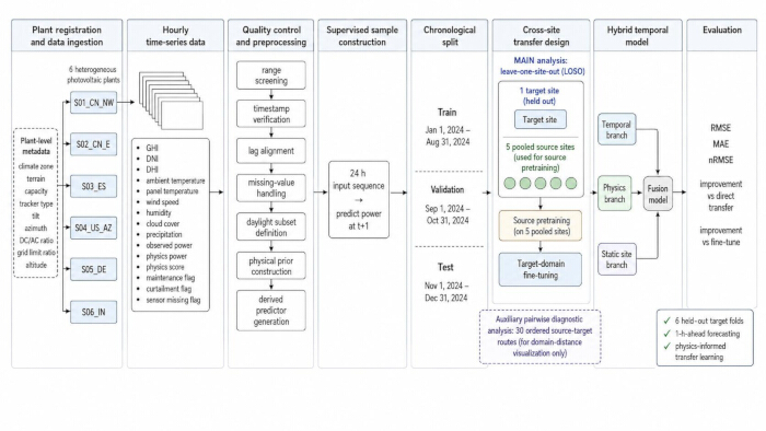
Figure 1: Overall workflow of the cross-site physics-informed transfer-learning framework. The workflow is read from left to right and summarizes six linked stages: plant and data registration; hourly quality control and preprocessing; physics-prior and feature construction; 24 h supervised sequence generation with chronological partitioning; pooled-source leave-one-site-out pretraining and target-site adaptation; and independent target-site evaluation with comparator, ablation, and statistical analyses. One plant is held out as the target in each of six folds, while the other five plants are pooled as the source domain. Abbreviations: PV = photovoltaic; TCN = temporal convolutional network; GRU = gated recurrent unit. Please click here to view a larger version of this figure.

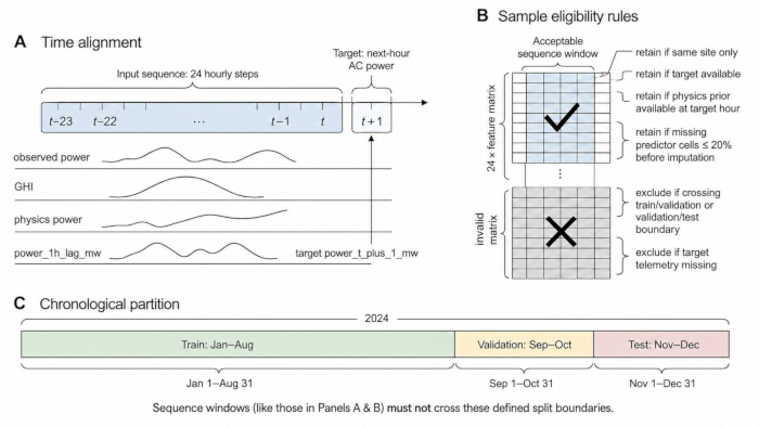
Figure 2: Time alignment, sample eligibility, and chronological segmentation for supervised sequence construction. (A) A 24 h input sequence from (t - 23) to (t) is used to predict next-hour alternating-current (AC) power at (t + 1). (B) Valid supervised samples must satisfy four conditions: site consistency, target availability, physical-prior availability, and missingness constraints. (C) The data are split chronologically into training, validation, and test subsets, and input windows crossing split boundaries are excluded. Abbreviations: AC = alternating current. Please click here to view a larger version of this figure.

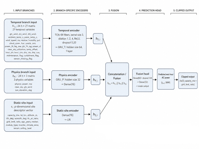
Figure 3: Architecture of the hybrid temporal model with temporal, physics, and static-site branches. The model combines a temporal branch for meteorological and operational sequences, a physics branch for physics-prior-related inputs, and a static-site branch for plant-level descriptors. The branch representations are concatenated and passed through the fusion head to generate the one-hour-ahead AC power prediction, which is constrained within the plant-specific export limit. Abbreviations: TCN = temporal convolutional network; GRU = gated recurrent unit; ReLU = rectified linear unit; GHI = global horizontal irradiance; DC = direct current; AC = alternating current. The temporal branch input is a 24 h × 21 matrix, whereas the physics branch input is a 24 h × 3 matrix; physics_power_mw, clear_sky_ghi_wm2, and sun_elevation_deg are assigned only to the physics branch and are excluded from the temporal branch. Please click here to view a larger version of this figure.

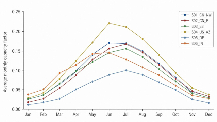
Figure 4: Monthly average capacity factors of the six photovoltaic plants. The figure presents the monthly mean capacity factors for each plant over the 12 calendar months from January through December 2024. The curves illustrate site-specific seasonal generation patterns and show that the six plants differ in both production level and seasonal timing. Please click here to view a larger version of this figure.

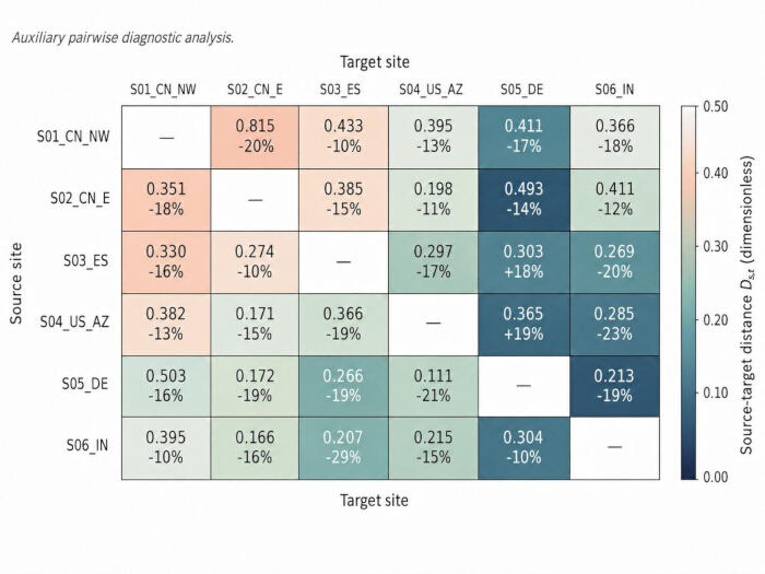
Figure 5: Pairwise source-target distance and relative transfer-improvement matrix. Please click here to view a larger version of this figure.

Each off-diagonal cell represents a single ordered source-to-target diagnostic route. The upper number is the dimensionless source-target distance D_s,t, where smaller values indicate greater similarity. The lower percentage is the relative change in RMSE for the full physics-informed transfer model compared with standard fine-tuning for that route; negative values indicate lower RMSE with the full model. This pairwise matrix is a secondary diagnostic analysis and is distinct from the six pooled-source target-fold results reported in Table 5. The color scale represents source-target distance and is dimensionless; it does not represent RMSE in MW. Abbreviations: RMSE = root mean squared error.

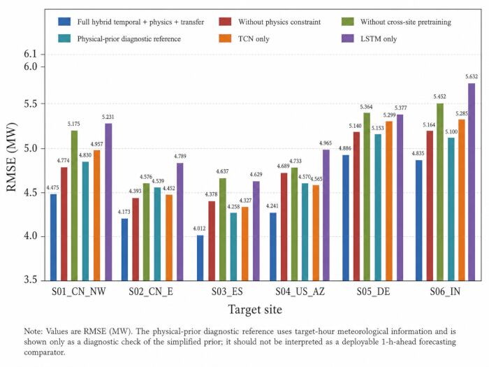
Figure 6: Target-wise ablation performance of the proposed forecasting model. The figure compares root mean squared error (RMSE) across the full model, matched ablation variants, and the physical-prior diagnostic reference for each target plant. The ablation results show the contributions of physics-informed consistency, cross-site pretraining, and the temporal encoder configuration. The physical-prior diagnostic reference uses target-hour meteorological information and is shown only as a diagnostic check of the simplified prior; it is not interpreted as a deployable one-hour-ahead forecasting comparator. Abbreviations: TCN = temporal convolutional network; LSTM = long short-term memory; RMSE = root mean squared error; MW = megawatt. Please click here to view a larger version of this figure.

Table 1: Static characteristics of the six photovoltaic plants included in the cross-site forecasting study. The table reports plant-level descriptors collected during site registration, including country, climate zone, terrain, installed capacity, direct-current/alternating-current ratio, tracker type, tilt, azimuth, geographical location, altitude, module type, inverter type, plant age, soiling level, and grid-limit ratio. These descriptors are used to document cross-site heterogeneity and to construct the static-site input branch. Please click here to download this Table.

Table 2: Variable definitions, units, data types, and preprocessing rules for predictors and labels. The table defines the static, dynamic, derived, and label variables used in the forecasting pipeline. It also specifies each variable’s modeling role and preprocessing rule, including plausibility screening, interpolation eligibility, scaling, encoding, clipping, and exclusion from imputation where applicable. For the 24 dynamic modeling predictors, the modeling role distinguishes 21 temporal-branch variables from the three physics-branch variables: physics_power_mw, clear_sky_ghi_wm2, and sun_elevation_deg. Please click here to download this Table.

Table 3: Training settings, transfer configurations, comparator models, and ablation conditions. The table summarizes the fixed methodological settings used in the six primary pooled-source leave-one-site-out folds and, where applicable, the separate 30-route pairwise diagnostic analysis. It includes forecast horizon, input sequence length, target variable, chronological split, feature scaling, categorical encoding, model architecture, optimizer settings, loss terms, comparator models, ablation variants, and performance metrics. The architecture specification uses a 24 h × 21 temporal input and a 24 h × 3 physics input, with mutually exclusive variable assignment between these two sequence branches. Please click here to download this Table.

Table 4: Site-level data quality and operational profile of the six photovoltaic plants. The table summarizes annual energy output, mean capacity factor, 95th percentile capacity factor, observed-power missingness, global horizontal irradiance missingness, curtailment frequency, maintenance frequency, sensor-flag rate, and the number of daylight test rows for each plant. Abbreviations: CF = capacity factor; p95 = 95th percentile; GHI = global horizontal irradiance; MWh = megawatt-hour. Please click here to download this Table.

Table 5: Target-wise forecasting performance in the six pooled-source leave-one-site-out folds. The table reports one performance summary for each held-out target plant. In each fold, the other five plants were pooled during source-stage pretraining. Metrics include RMSE for local-only, direct-transfer, fine-tuning, and full-model settings, as well as full-model MAE, normalized RMSE, and relative improvement over fine-tuning and direct transfer. Any source-target distance column is a descriptive context based on the five pairwise distances entering that target and is not the basis for averaging the forecasting-performance columns. The physical-prior value, if shown, is a target-hour diagnostic of the simplified prior rather than an operational one-hour-ahead forecasting comparator. Please click here to download this Table.

Table 6: Target-wise ablation results of the proposed forecasting model. The table compares RMSE values for the full hybrid temporal physics-informed transfer model, matched ablation variants, and the physical-prior diagnostic reference at each target plant. The ablation conditions evaluate the effects of removing the physics constraint, cross-site pretraining, and simplifying the temporal encoder. The physical-prior diagnostic reference is reported separately and is not interpreted as an operational one-hour-ahead forecasting comparator. Please click here to download this Table.

Discussion

This study evaluated a cross-site physics-informed transfer-learning framework for one-hour-ahead photovoltaic power forecasting across heterogeneous solar plants. In the primary six-fold leave-one-site-out experiment, the full hybrid temporal model combined pooled-source pretraining, target-site fine-tuning, plant-level static descriptors, and a physics-informed loss component, achieving the lowest forecasting error across all held-out target plants. This finding supports the use of hybrid photovoltaic forecasting models that combine machine-learning-based temporal representations with physically meaningful prior knowledge⁹. Importantly, the method improved cross-site generalization without eliminating inherent differences in forecasting difficulty among plants. S05_DE remained the most difficult target, whereas S04_US_AZ remained the easiest target according to the primary evaluation metrics, suggesting that the framework reduced prediction error while preserving site-specific operating complexity.

The results also showed that transfer learning alone was insufficient for reliable photovoltaic forecasting across sites. Direct transfer performed worse than target-site fine-tuning, indicating that source-domain knowledge required adaptation before it could be reliably applied under different climatic, geographical, or engineering conditions. This pattern is consistent with evidence that photovoltaic power prediction is sensitive to plant configuration, environmental conditions, and site-level operating constraints, even when a unified modeling strategy is applied across multiple locations¹⁰. A model trained at one site may capture transferable temporal features; however, these features may require adjustment when the target plant differs in installed capacity, tracking system, module type, soiling condition, or grid export limit.

The added value of the proposed framework appeared to arise from the joint use of temporal feature extraction, pooled-source transfer, target-site adaptation, and plant-specific physical constraints. Removing the physics-consistency term increased forecasting error, while removing source-domain pretraining resulted in a further loss of performance. The simplified physical prior also showed nontrivial agreement with observed target-hour power, although its direct diagnostic error remained higher than that of the full model. Because the diagnostic prior used target-hour meteorological information and the clear-sky-normalized irradiance ratio could remain high at low solar elevations, it should not be interpreted as a deployable one-hour-ahead forecast. Instead, its role in the proposed framework was to provide a low-weight soft inductive bias. Future studies should prospectively compare this formulation with absolute-irradiance or clear-sky-power-profile priors using forecast-available meteorological inputs.

The framework remained relevant for cross-site adaptation because pooled source-domain pretraining provided an informed initialization prior to target-specific updating. Because the final analysis used the complete eligible target-site training subset rather than prespecified fractional subsets, the present results supported cross-site transfer and target adaptation under the fixed 2024 training period but did not constitute a quantitative few-shot learning curve. Future studies should explicitly compare prespecified target-data fractions and evaluate how transfer gains change as local historical data accumulate.

From a deployment perspective, the proposed network was relatively compact, with approximately 6.67 × 10⁴ trainable parameters per model and a fixed 24-step input. This architecture is materially smaller than contemporary general-purpose time-series foundation models. The compact architecture may therefore be advantageous when plant operators require site adaptation without foundation-model-scale computational resources. However, device-specific inference latency was not archived in the present study; therefore, computational characterization was limited to model size and operation count rather than an exact real-time benchmark. Future deployment studies should report standardized batch-1 inference latency, throughput, memory consumption, and energy use on the intended edge or control-room hardware.

Several limitations should be noted. First, the study covered only one calendar year, and the independent test period was fixed to November and December 2024. The reported performance may therefore partly reflect season-specific irradiance, cloud, and operating conditions, and broader multi-year testing is required before year-round stability can be inferred. Second, the study did not include a target-data-fraction sensitivity analysis and therefore did not quantify how the transfer benefit changed jointly with target sample size and seasonal coverage. Third, the physical prior was deliberately simplified, and its direct diagnostic used target-hour meteorological information; therefore, it should not be interpreted as an operational one-hour-ahead forecast. Alternatives based on forecast-available irradiance or clear-sky power should be evaluated prospectively. Fourth, the physics-consistency and boundary-loss weights were fixed at 0.20 and 0.05, respectively, and a formal sensitivity analysis was not performed. Fifth, complete per-seed dispersion statistics were not retained in the summary outputs; therefore, interquartile ranges and standard deviations could not be reported. Sixth, maintenance/curtailment-filtered and weather-stratified robustness analyses were not included in the final analysis, while source-target mismatch was examined only descriptively through the secondary pairwise diagnostic analysis. Seventh, the comparator set did not include transformer or foundation-model architectures; therefore, the study should not be interpreted as establishing superiority over all contemporary forecasting models. Eighth, although the source records were actual measured plant observations, the de-identified analytical workbook did not retain complete upstream acquisition metadata for every source-record variable; this limits independent verification at the site-owner, sensor-vendor, and platform levels. Ninth, hardware-specific inference latency and the exact original CPU/GPU models were not retained. Finally, although the six plants were deliberately heterogeneous, they were not a probability sample of the global photovoltaic fleet. Validation across additional years, climates, plant sizes, tracking designs, equipment types, and grid-control regimes is therefore needed to strengthen generalizability.

Overall, the findings supported the integration of pooled-source transferable temporal representations, target-site adaptation, site-level descriptors, and physically constrained learning within the six-site, one-year evaluation considered here. The primary evidence was derived from six held-out-target leave-one-site-out folds, while the 30 ordered source-target routes provided a separate diagnostic analysis of transfer heterogeneity. The findings should therefore be interpreted as evidence supporting this integrated strategy under the reported dataset and evaluation design rather than as proof of universal superiority across all photovoltaic forecasting settings.

Materials

List of materials used in this article

Name	Company	Catalog Number	Comments
CUDA-enabled GPU computing environment	NVIDIA Corporation	CUDA-compatible workstation environment	Used to accelerate deep-learning model training and evaluation.
Integrated development environment	Microsoft Corporation	Visual Studio Code	Used for code development and workflow management.
Matplotlib	Matplotlib Development Team	Matplotlib 3.9.2	Used for scientific visualization and figure generation.
NumPy	NumPy Developers	NumPy 1.26.4	Used for numerical computation and array-based data processing.
Pandas	pandas Development Team	pandas 2.2.3	Used for tabular data loading, cleaning, transformation, and dataset preparation.
Python programming language	Python Software Foundation	Python 3.11.9	Used for data preprocessing, model training, evaluation, and reproducibility workflows.
PyTorch deep learning framework	PyTorch Foundation	PyTorch 2.5.1	Used for implementation and training of temporal, physics, and static-site neural network branches.
Scikit-learn	scikit-learn Developers	scikit-learn 1.5.2	Used for preprocessing utilities, scaling, encoding, and statistical evaluation support.
Spreadsheet software	Microsoft Corporation	Microsoft Excel	Used for data organization, table preparation, and manuscript supplementary materials.
Version control system	Git	Git 2.x	Used for code version management and reproducibility.

References

- Di Leo P, Ciocia A, Malgaroli G, Spertino F. Advancements and challenges in photovoltaic power forecasting: a comprehensive review. Energies. 2025;18:2108.
- Husein M, Gago EJ, Balfaqih H, Pegalajar MC. Towards energy efficiency: a comprehensive review of deep learning-based photovoltaic power forecasting strategies. Heliyon. 2024;10:e33419.
- Tang Y, Yang K, Zhang S, Zhang Z. Photovoltaic power forecasting: a hybrid deep learning model incorporating transfer learning strategy. Renew Sustain Energy Rev. 2022;162:112473.
- Luo X, Zhang D, Zhu X. Combining transfer learning and constrained long short-term memory for power generation forecasting of newly-constructed photovoltaic plants. Renew Energy. 2022;185:1062-1077.
- Wen Y, et al. Improving multi-site photovoltaic forecasting with relevance amplification: DeepFEDformer-based approach. Energy. 2024;299:131479.
- Jang SY, Oh BT, Oh E. A deep learning-based solar power generation forecasting method applicable to multiple sites. Sustainability. 2024;16:5240.
- Paletta Q, Nie Y, Saint-Drenan YM, Le Saux B. Improving cross-site generalisability of vision-based solar forecasting models with physics-informed transfer learning. Energy Convers Manag. 2024;309:118398.
- Depoortere J, Driesen J, Suykens J, Kazmi HS. SolNet: open-source deep learning models for photovoltaic power forecasting across the globe. Int J Forecast. 2025;41:1223-1236.
- de Oliveira Santos L, AlSkaif T, Barroso GC, de Carvalho PCM. Photovoltaic power estimation and forecast models integrating physics and machine learning: a review on hybrid techniques. Sol Energy. 2024;284:113044.
- Zhang L, Wilson R, Sumner M, Wu Y. Transfer learning in very-short-term solar forecasting: bridging single site data to diverse geographical applications. Appl Energy. 2025;377:124353.
- Cong Z, Chen Y, Wang Z, Zhang D. Physics-informed day-ahead PV power forecasting with seasonal trend mitigation and clear-sky template integration. Energy 360. 2025;4:100035.
- Liu W, Mao Z. Short-term photovoltaic power forecasting with feature extraction and attention mechanisms. Renew Energy. 2024;226:120437.
- Sarmas E, et al. Transfer learning strategies for solar power forecasting under data scarcity. Sci Rep. 2022;12:14643.
- Lyu C, Eftekharnejad S. Probabilistic solar generation forecasting for rapidly changing weather conditions. IEEE Access. 2024;12:79091-79103.
- Bellagarda A, et al. Effectiveness of neural networks and transfer learning to forecast photovoltaic power production. Appl Soft Comput. 2023;149:110988.
- Miraftabzadeh SM, Colombo CG, Longo M, Foiadelli F. A day-ahead photovoltaic power prediction via transfer learning and deep neural networks. Forecasting. 2023;5:213-228.
- Liao R, et al. Enhanced photovoltaic power generation forecasting for newly-built plants via physics-infused transfer learning with domain adversarial neural networks. Energy Convers Manag. 2024;322:119114.
- Ma T, et al. Short-term photovoltaic power forecasting based on a new hybrid deep learning model incorporating transfer learning strategy. Glob Energy Interconnect. 2024;7:825-835.
- Das A, Kong W, Sen R, Zhou Y. A decoder-only foundation model for time-series forecasting. Proceedings of the 41st International Conference on Machine Learning. 2024;235:10148-10167. https://proceedings.mlr.press/v235/das24c.html
- Goswami M, et al. MOMENT: a family of open time-series foundation models. Proceedings of the 41st International Conference on Machine Learning. 2024;235:16115-16152. https://proceedings.mlr.press/v235/goswami24a.html
- Yousuf KB, et al. A hybrid XGBoost-LSTM model with physics-informed features and uncertainty quantification for solar power forecasting. Energy Rep. 2026;15:109068.