Gated-Slot Linear Attention Graph Neural Networks for Session-based Recommendation

Summary

This paper proposes a novel model, gated-slot linear attention graph neural networks for session-based recommendation, which adopts gated-slot linear attention based on a dual-constructed session graph. It boosts recommendation accuracy and efficiency and outperforms SOTA on three public datasets.

Abstract

Session-based Recommendation (SBR) systems aim to predict the next item which a user is likely to interact with, based on behavior sequence within the current session. Recent approaches leveraging the Transformer attention mechanism (e.g.,GC-SAN) have demonstrated superior performance over traditional methods; however, they suffer from heavily computation workload and space complexity due to the quadratic cost of self-attention. To address these limitations, a novel model termed GSLA4Rec (gated‑slot linear attention graph neural networks for session‑based recommendation) is proposed, which integrates linear attention with a learnable gating mechanism and a slot‑based memory update strategy inspired by gated‑slot attention. Specifically, GSLA4Rec first constructs two graphs: session graph to capture intra-session item transitions and neighbor global graph to encode cross-session collaborative signals, thereby modeling both local and global context information. The proposed approach centers on the gated-slot linear attention mechanism, which (1) employs gating units to suppress noise from irrelevant or redundant interactions in long sessions, (2) utilizes slot units to dynamically store and update compact session representations—reducing memory overhead, and (3) replaces self-attention with linear attention to achieve linear-time complexity. Together, these components significantly enhance the model’s predictive accuracy and efficiency in capturing evolving users’ interests. Extensive experiments on multiple public benchmark datasets, including Diginetica, Tmall, and NowPlaying, demonstrate that GSLA4Rec consistently outperforms SOTA SBR methods in recommendation performance, which validates the effectiveness of GSLA mechanism.

Introduction

With the rapid development of online services (such as e-commerce, short video platforms, and news feeds), the issue of information overload has grown increasingly prominent and severe. Recommender systems^1,2provide personalized and precise information push services by deeply analyzing users’ behavior data. However, in many practical applications characterized by anonymous access, unlogged users, privacy protection, and short interaction durations, traditional recommendation methods such as collaborative filtering³and matrix factorization^4,5 greatly limit the applicability of recommendation algorithms. To address these challenges, SBR^6,7,8,9 has emerged. SBR focuses on the interaction sequence data within users' current session to predict the next potential point of interest. This paradigm not only avoids reliance on long-term users’ history data but also keenly captures short-term dynamic interest changes, thus demonstrating unique application value in scenarios like e-commerce, short videos, music recommendation and so on.

Early methods primarily relied on Markov Chains^5,10,11,12 to model transition probabilities between items in session sequences. Although these methods could capture first-order sequence dependencies, the characterization of complex high-order dependencies and nonlinear dynamics of user interests remains limited, restricting model effectiveness in complex scenarios. With the development of Deep-Learning technology^13,14, neural network-based methods have been widely applied in the SBR. GRU4REC¹⁵was the first to apply recurrent neural networks¹⁴ (RNNs) to session-based recommendation, effectively capturing temporal dependencies in sequences; NARM¹⁶further enhanced the ability to mine core users’ interests by integrating attention mechanisms with RNNs; STAMP¹⁷ utilized multi-layer perceptrons (MLPs) combined with attention mechanisms to focus on capturing short-term users’ interests. While these methods achieved some progress in sequence modeling, they still faced challenges such as difficulty in handling long-term dependencies and sensitivity to noise.

In recent years, Graph Neural Networks (GNNs)^18,19,20,21have brought a new perspective to the SBR task. Models such as SR-GNN²²explicitly model complex transition relationships by constructing session graph (SG), achieving substantial improvements in recommendation accuracy. However, most existing GNN-based methods conduct graph construction and message passing within individual sessions, lacking effective utilization of global item correlation information. To address this issue, GCE-GNN²³integrates global semantics and session graphs with a self-attention mechanism to adaptively weigh item importance by constructing neighbor global graph (NGG), achieving considerable performance improvements. Nevertheless, existing GNNs-based methods still face two major bottlenecks: First, the complexity of the self-attention mechanism grows quadratically with session length, resulting in substantial computational overhead when processing long sessions; Second, traditional GNNs lack the ability to dynamically regulate item importance during information aggregation, making it difficult to distinguish between noise and critical behaviors, which affects representation quality.

To address these challenges, this paper proposes a gated-slot linear attention graph neural network for session-based recommendation (GSLA4Rec): (1) Designing a gated-slot mechanism that filters noise via gating and stores key semantic information in session slots, enhancing the model's robustness and reducing storage overhead; (2) Introducing the linear attention mechanism that reduces computational complexity from O(N²) to O(N) where N is the session length), while maintaining the ability to model long-distance dependencies; (3) Conducting extensive experiments on three public benchmark datasets (Diginetica, Tmall, and NowPlaying), showing that GSLA4Rec significantly outperforms existing SOTA methods, especially demonstrating clear advantages in long-session and sparse scenarios.

Protocol

Experiencing session-based recommendation

Session‑based recommendation could be examined from three perspectives: SBR, global context learning, and GSLA (refer to Table of Materials). No human participants or animals were involved in this study. All experimental datasets used in this work are publicly available and submitted as Supplementary File: GSLA4Rec. zip.

Session-based recommendation

The session-based recommendation (SBR) was an artificial intelligence system that interacted with users through multi-turn natural language dialogues to dynamically understand users’ preferences and provide personalized recommendations. SBR evolved from traditional methods to deep learning-based and hybrid approaches, and then advanced towards Large Language Model (LLM)-based solutions.

Traditional session-based recommendation

Traditional SBR was typically represented by Markov Chain-based methods and Collaborative Filtering. The former generated recommendations by decomposing user-specific probabilistic transition matrices. For instance, Guy Shani²⁴ proposed a Markov Decision Process-based recommendation method that produced recommendations by decomposing corresponding matrices; Wanrong Gu²⁵ enhanced recommendation performance by integrating Markov Chains with purchase time intervals. The latter generated recommendations by extracting hidden sequential relationships between adjacent interactive items through matrix factorization. For example, Sarwar B¹ calculated item-to-item similarity based on users’ historical behaviors (such as score and clicks) to recommend items that match users’ past preferences. If user A liked item a, and item c was highly similar to a, the system recommends c to A; Rendle S⁵ proposed FPMC, a sequence recommendation model combining matrix factorization with Markov Chains, to capture hidden sequential relationships between adjacent interactive items. However, such traditional SBR focused on sequential relationships between adjacent items, making it difficult to model complex dependency relationships.

Deep-learning session-based recommendation

Deep-Learning session-based recommendation had evolved through stages involving Convolutional Neural Networks (CNNs)^26,27,28,29, RNNs, and GNNs. CNN-based SBR utilized operations such as convolution and pooling to learn representations of each session context, which then used for subsequent recommendations. Caser³⁰ converted the L most recent items that a user had interacted with into d-dimensional vectors via an embedding layer, forming an embedding matrix treated as an "image" mapped in time and latent space. It then used three sequence pattern convolutional filters—point-level, union-level with no skip, and union-level with skip once—to learn sequential patterns for better SBR performance. Tuan et al.³¹ uniformly modelled session click streams and content features via 3D convolution kernels to form spatio-temporal-content joint representations.

RNNs were a class of neural network architectures specifically designed to process sequential data. The core idea was to capture temporal dependencies through recurrent structures such as long short-term memory networks (LSTM)¹³ and gated recurrent units (GRUs)³², and they were widely used in fields such as natural language processing (NLP)³³, speech recognition³⁴, text translation³⁵, travel^36,37, crime³⁸, and future trend prediction³⁹ (e.g., traffic⁴⁰, stock markets^41,42, and meteorology⁴³). GRU4Rec, proposed by Hidasi et al., was a milestone in SBR research, and it first introduced RNNs into SBR and captured users' sequential behavioral patterns via GRU for achieving personalized recommendations.

GNNs⁴⁴ demonstrated strong expressive power in modeling complex relationships within graph-structured data, and some researchers introduced GNNs to model complex transitions within or between sessions. Depending on different GNNs model architectures, GNNs-based methods for SBR were generally categorized into gated graph neural networks (GGNNs)⁴⁵, graph convolutional networks (GCNs)⁴⁶, and graph attention networks (GATs)⁴⁷. SR-GNN was the first to apply GNNs to SBR by representing session sequences as directed graphs and utilizing GGNNs to capture complex item transition relationships within sessions, combined with attention mechanisms to obtain the final session embedding, thereby improving recommendation performance. Chen L⁴⁸ proposed a multi view GNNs framework that combines structured attributes and unstructured keywords to model multi-dimensional product associations, improving the accuracy of SBR. Driss E⁴⁹ designed an innovative session recommendation system adopting capsule graph neural networks to capture complex item features and enhance prediction accuracy for SBR.

The aforementioned deep-learning techniques had enriched the research scope of SBR and effectively improved performance, yet they still had certain limitations, mainly manifested in: 1) For newly emerging items or very sparse sessions, it was difficult for the models to make accurate predictions due to the lack of global context; 2) They couldn't leverage the global patterns contained in all historical sessions.

Hybrid session-based recommendation

Hybrid session-based recommendation integrated the strengths of different techniques, such as collaborative filtering, Deep-Learning, and attention mechanisms, to improve SBR performance. GC-SAN⁵⁰ incorporated a self-attention mechanism based on SR-GNN to better capture interaction information of important items within a session. FGNN⁵¹ further aggregated information from neighboring items through a multi-head attention mechanism to learn multiple relationships of the target item. SR-HetGNN⁵² belonged to SBR with heterogeneous graphs; by introducing multi-type items (user, item, session) and multi-relational edges (click, purchase, co-occurrence, attribute association), it constructed a global knowledge network, breaking through the limitation of single item sequences, and was an important method for modeling anonymous users’ behavior and cross-session interest associations in recent years. KGSR-SAP⁵³ constructed a knowledge graph by connecting items with edges of multiple relationships to describe various user-item interactions, solving the information loss problem where the global graph only contains edges of one type (user-item interaction). Wang ZH⁵⁴ proposed DiffSBR, a diffusion-based session recommendation model. It generates reliable next-item preferences by simulating noise denoising, improving modeling of dynamic user click sequences. Qiao ST⁵⁵ builded a SBR framework combining multi-view intent learning and LLM alignment. It mined user implicit intent from diverse perspectives and leveraged language models to align semantic features for better improving recommendation performance.

Global context

To overcome the shortcoming of "viewing sessions in isolation", researchers realized that global information could be used to enhance the representation capability of the current session, so as to solve problems such as data sparsity, cold start, and semantic gap in traditional SBR. Meanwhile, when constructing global context, integrating global information into a single session while minimizing noise interference was required. CSRM⁵⁶ optimized session-level representation by integrating collaborative information between the current session and neighboring sessions, using an outer memory encoder (OME) to extract collaborative intent from the collaborative information. CA-TCN⁵⁷ proposed a cross-session aware temporal convolutional network model, constructing global graphs and session context graphs to simulate the impact of cross-session on items and sessions, while the temporal convolutional network (TCN) expands the receptive field through dilated convolutions, with the number of layers covering sequences of exponential length (receptive field = ), solving the gradient vanishing problem of RNNs. Chen⁵⁸ proposed a SBR method based on hypergraph neural networks (SR-HGNNs), which integrates mixed-order (low-order and high-order) propagation and attention mechanisms to solve the over-smoothing problem of traditional GNNs in short sessions and distinguish the importance of different propagation orders, and could more accurately capture dependencies and avoid noise interference. GCE-GNN used multi-order co-occurring item pairs to construct an undirected weighted graph, counting item co-occurrence frequencies to reflect the importance of items in the session; AGNN-GC⁵⁹ used cross-session item transition relationships to construct a global collaborative graph, calculating item transition probabilities in the global graph to reflect interest changes in the session; DA-GCN⁶⁰ used the shortest path to update the adjacency matrix to construct a dynamic weighted graph, calculating global graph co-occurrence frequency and path distance between items. Inspired by the above literature, this paper proposed constructing a global graph through a neighbor-based method, i.e., using the Jaccard similarity coefficient to calculate similar sessions, which not only utilized global information but also filtered noise (filtering out irrelevant items), achieving the purpose of accurately constructing global context and laying a solid foundation for the subsequent SBR algorithm.

Gated-slot linear attention

Traditional transformers⁶¹ incured high spatiotemporal complexity due to the need for fully connected attention operations across the entire sequence as follows:

(1)

Where Q, K, V ∈ R^N×d were linear transformations of the input items, M = {M_ij = 1 if i ≥ j, o.w. −∞ } was the causal mask to prevent future information leakage, ⊙ denoted element-wise production, and f denoted the activation function softmax.

To achieve linear attention⁶², the most direct idea was to remove the activation function softmax. However, if the activation function softmax was directly removed, linear attention would definitely lead to some potential problems: Losing the powerful expressive power of neural networks and being unable to solve complex real-world problems.

Slot linear attention with bounded-memory control

Assuming the activation function softmax needed to be retained, K and V were compressed separately into K̃, Ṽ ∈ R^m×d. From the perspective of memory network, K̃ and Ṽ had memory slots whose length increases with the sequence, that is, the number of slots m = N. If m was fixed, linearization was obviously possible. Inspired by Bounded-memory Control⁶³, each token in the input items with a length of N was required to be competitively written into m slots.

,, (2)

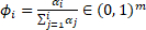
Where f was the activation function softmax and φ_i was vector to control effective input for controlling key value k_i as follows.

, (3)

Here, (φ_i)_j represented the writing intensity of the ith token to the jth slot, was obtained using a cumulative softmax function.

To achieve efficient linear computation, formula (2) was rewritten as formula (4), which computed ο_i from q_i, k_i, and v_i (Eq. 4) by {ο_i|_i=1^T, q_i, k_i, v_i)|_i=1^T} and adopted two-pass sequential computation:

, (4)

Hence SLA operations could be derived:

,  (5)

Where o_i′ ∈ ℝ^m, ο_i ∈ ℝ^d. Therefore, SLA could acquire hardware-efficient linear-time chunk-wise training⁶⁴.

Gated-slot linear attention

Slot linear attention with bounded-memory control could reduce computational and spatial complexity. However, the accumulation of information could also bring noise information into session interaction, so data-dependent decay was very important for selectively retaining and forgetting information, and this selective mechanism had been revisited in recent selective state-space models⁶⁵. GSLA with data-dependent could be expressed as:

,  (6)

Here decay gates were parameterized by an outer product form G_i = α_i ⊗ β_i, α_i, β_i ∈ [0,1]^d. In what follows, GSLA could also be written in the following equivalent form by typically setting β_t = 1 and matrix multiplication as in⁶⁴:

(7)

Where α_i and k_i separately denoted forget gate and input gate, the two gates could be coupled as k_i = 1 − α_i, inspired by the literature on gated RNNs. It was evident that GSLA could be formulated with two‑pass sequential computation as shown in Equation (8). The second-order structure supported block parallel training to improve training efficiency, and the insertion of softmax operation in the middle of the second-order structure enhanced the modeling ability of finite slot memory.

,
(8)

Transforming session data

Problem definition

Let the given session sequence be S = {v₁^s, v₂^s, ⋯, v_n^s}, where v_i^s denoted the ith clicked item. By analyzing the user's click behavior within this sequence, the system predicted the next item the user may be interested v_n+1^s.

Graph construction

Session graph construction

For a session S = {v₁^s, v₂^s, ⋯, v_n^s}, a directed graph G_s = (V_s, ε_s) was constructed, where V_s was the item set of the given session S, and ε_s = {e_ij^local|v_i, v_j, v_i, v_j ∈ V_s} was the edge set of the given session S. ε_{(vi-1^s, vi^s)} represented the consecutive clicked items in this session. The edge e_ij^local could be divided into four types: e_in, e_out, e_in-out, e_self. Since the same item might appear repeatedly in the sequence, the weighted value for each edge was counted.

The current session s = [v₁, v₂, v₄, v₂, v₃] was converted into an SG, as shown in Figure 1A.

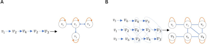
Figure 1: Transform interactive items into graph structures. (A) Illustration of session graph (SG) construction by transforming a session into a graph. (B) Illustration of neighbor global graph (NGG) construction by combining many sessions into a graph. This figure was self-drawn via Visio with fully customized elements. No copyrighted external graphic resources were used, hence no additional third-party copyright licensing was needed. Figure copyright was owned by the authors and would comply with the journal's copyright rules upon acceptance. Please click here to view a larger version of this figure.

Neighbor global graph construction

Based on the current session S, the corresponding NGG G_g = (V_g, ε_g) was constructed to enrich the representation learning of the current session in a cross-session manner. V_g was the item set containing all items in G_g, and ε_g = {e_ij^global|v_i, v_j, v_i, v_j ∈ V_g} was the edge set of G_g. ε_{(vi-1^g, vi^g)} represented the directly interacting items v_i-1^g and v_i^g in the NGG G_g. This process consisted of two steps: neighbor session acquisition and NGG construction.

Neighbor session acquisition

Across the entire dataset, sessions with the maximum number of co-occurring items with the current session were searched. The top-N sessions with the highest co-occurrence counts were selected to construct a candidate neighbor session set S. Subsequently, the Jaccard similarity coefficient was employed to calculate the similarity between the current session c_u and a session S_r ∈ S from the candidate set S, as shown in Equation (9).

(9)

Here, co(S_c^u, S_r) denoted the number of items co-occurring in both S_c^u and S_r, while l(S_c^u) and l(S_r) respectively represented the lengths of S_c^u and S_r, and S_c^u and S_r denoted current session and a neighbor session. Sessions with similarity below a certain threshold (which could be set as a hyperparameter) were filtered out, and the remaining sessions constituted the neighbor session set N_s for the current session.

Neighbor global graph construction

Based on the neighbor session set N_s, the NGG was constructed, as illustrated in Figure 1B. During the adjacency matrix construction, if two items (v_i, v_j) had an interaction, the corresponding entry A_ij was set to 1, otherwise, it was set to 0. Additionally, the interactions between items were processed as undirected and were equipped with self-loops, followed by normalization, as shown in Table 1.

	1	2	3	4	5	6
1	1/2	1/2	0	0	0	0
2	0	1/4	1/4	1/2	0	0
3	0	0	1	0	0	0
4	0	1/4	1/2	1/4	0	0
5	0	0	0	0	1/3	2/3
6	0	1/3	0	1/3	0	1/3

Table 1: Normalized adjacency matrix of the neighbor global graph. The table presents the normalized adjacency matrix describing the weighted connections among nodes in the constructed neighbor global graph.

Designing session-based recommendation algorithm

This section elaborates on the proposed innovative model GSLA4Rec, which enhanced SBR performance by introducing the GSLA mechanism over the joint feature representation of SG and NGG.

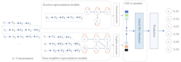
Figure 2: GSLA4Rec framework. This framework integrated session graph and neighbor global graph structure learning, filtered interaction noise with a gating mechanism, balanced storage and efficiency with a memory slots mechanism, and captured item relevance with a linear attention mechanism to predict the user's next click preference. This figure was self-drawn via Visio with fully customized elements. No copyrighted external graphic resources were used, hence no additional third-party copyright licensing was needed. Figure copyright was owned by the authors and would comply with the journal's copyright rules upon acceptance. GSLA4Rec represented gated-slot linear attention graph neural networks for SBR. Please click here to view a larger version of this figure.

Figure 2 presented the framework of GSLA4Rec, which comprised four main components: 1) Session-level item representation. It employed a GNNs model on SG to learn session-level item embeddings within the current session; 2) Neighbor global-level item representation. It learned global-level item embeddings over all sessions by employing a GRU to recursively incorporate the neighbor embeddings of each item based on the NGG; 3) GSLA. It modelled the users’ preference of the current session by aggregating the learnt item representations at both session-level and global-level; 4) Prediction layer. It outputed the predicted probabilities over candidate items. The four components were presented in detail in the following.

Session representation

In SBR, understanding users’ interaction behaviors was crucial. To this end, a SG and a NGG were constructed for session representation learning, aiming to comprehensively understand users’ interaction behaviors and thereby capture the users’ more authentic intent.

Session-level item representation

Based on the SG in Figure 1A, a Weighted Bidirectional Graph Attention (WBGAT) method was employed to extract features of the SG. This method introduced edge weights and item directionality (In-neighbor and Out-neighbor) based on the standard GAT mechanism, achieved the effect of strengthening important edges and capturing bidirectional dependencies, thereby addressed the shortcomings of traditional GAT regarding asymmetric item relationships and interaction strength. The calculation process was as follows:

First, calculation of item in-degree normalization weights.

(10)

where e_ij indicated the first-order in-neighbor weight of item j’s features to item i,  was the relation between item i and item j, β^* ∈ ℝ^d was weight vectors, h_i and h_j was respectively representation of item i and j, W_i⁽ⁱⁿ⁾ ∈ ℝ^d*d and W_j⁽ⁱⁿ⁾ ∈ ℝ^d*d were trainable parameters, || represented concatenation operation. To distinguish different in-degree relations, two weight vectors, namely r_in and r_in-self, were trained. LeakyReLU was adopted as the activation function.

(11)

To make coefficients comparable across different items, the attention weights were normalized via the softmax function. Where N_i⁽ⁱⁿ⁾ was the first-order in-neighbor set of item i,  was the in-neighbor weight of directed edge (i←j) in SG, this method enabled the model to learn item feature correlations while retaining the inherent connection strength information of the graph structure by taking the logarithm of the edge weights and adding them to the original attention score e_ij.

Second, calculation of item out-degree normalization weights.

(12)

where ẽ_ij indicated the first-order out-neighbor weight of item j’s features to item i,  was the relation between item i and j, two weight vectors, namely r_out and r_out-self, were trained.

(13)

Where N_i^(out) was the first-order out-neighbor set of item i, was the out-neighbor weight of directed edge (i→j) in SG.

Third, information aggregation. The updated embedding of item could be obtained after weighting and summing the first-order in-degree and out-degree embeddings of item i.

(14)

Where  and α̃_ij respectively denoted in-degree and out-degree weights of item i, denoted the updated representation of item i.

Neighbor global-level item representation

Recent research consistently agreed that constructing a global graph could enhance data representation and thereby improve SBR performance, this was beyond doubt. However, globally enhancing data might also introduce irrelevant information such as noise. In the proposed model, to achieve global data augmentation while minimizing noise to the greatest extent possible, a near-neighbor global graph was constructed.

Based on the NGG in Figure 1B and the normalized adjacency matrix in Table 1, the current session and its neighbor sessions were transformed into an NGG, and a GGNNs⁴⁵ method was applied to extract features of the NGG. The learning process of item vectors in the NGG was shown in Equation (15).

(15)

W ∈ ℝ^d×2d denoted control weights, z_g,i and r_g,i represented the update gate and reset gate, respectively. [h₁^t-1, ⋯, h_n^t-1] represented the list of all item vectors in session s. σ(x) = 1/(1 + e^-x) was the logistic sigmoid function, ⊙ denoted element-wise multiplication, and h_i ∈ ℝ^d represented the vector after gated updating. The adjacency matrix A_s ∈ ℝ^n×n indicated the connectivity between items in neighboring sessions, and A_s,i: ∈ ℝ^1×n represented a column block A_s corresponding to item v_s,i in the adjacency matrix. For the current session s = [v₁, v₂, v₄, v₂, v₃], the NGG and the normalized adjacency matrix were shown in Figure 1B and Table 1, respectively.

Item representation

The item representation was obtained by summing the session-level item vector and the neighbor global-level item vector, as shown in Equation (16):

(16)

Where dropout was utilized on global-level neighbor item representations to alleviate overfitting.

Gated-slot linear attention

The gated-slot linear attention (GSLA) in this paper integrated linear attention with bounded-memory control and a data-dependent gating mechanism. On one hand, it inherited the finite memory slot mechanism of the attention-based controller (ABC) model, compressed key-value pairs that originally grew with sequence length into a fixed number of slots, and each slot was updated via competitive writing, addressing the computational complexity issue of transformer global attention. On the other hand, it introduced a fine-grained gating mechanism similar to GLA, where input data dynamically adjusted the retention ratio of historical information through a forget gate α_i, resolving the noise problem caused by the lack of a forgetting mechanism in ABC.

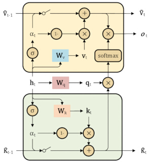
Figure 3: Schematic diagram of GSLA. The input vector was mapped to the query vector, keyword vector, and value vector, respectively, and then processed by linear attention with bounded-memory control and a data-dependent gating mechanism to obtain the updated query vector, keyword vector, value vector, and output vector. This figure was self-drawn via Visio with fully customized elements. No copyrighted external graphic resources were used, hence no additional third-party copyright licensing was needed. Figure copyright was owned by the authors and would comply with the journal's copyright rules upon acceptance. GSLA represented gated-slot linear attention. Please click here to view a larger version of this figure.

As specifically implemented in Figure 3, the input vector was separately mapped into the query vector, key vector, and value vector⁶⁴:

(17)

Where W_q, W_k, W_v ∈ ℝ^d×d represented the transformation weight matrices respectively corresponding to the query, key, and value, and h_t denoted the embedding vector at the tth time step in the session input sequence. The Swish function was defined as Swish(x) = x · σ(x) and was a self-gated activation function, where σ was the Sigmoid function, it outperformed the traditional ReLU activation function in multiple Deep-Learning tasks.

GSLA utilized a forget gate α_i and an input gate 1 − α_i, depending on input data, to dynamically update the information in the ith memory slot. The process was as follows⁶⁴:

(18)

(19)

Here, K̃_t and Ṽ_t represented the key vector slots and value vector slots at time step t, while K̃_t-1 and Ṽ_t-1 represented the key vector slots and value vector slots at time step t−1. The forget gate α_i = σ(W_αh_t)^1/τ, where W_α ∈ ℝ^d was the transformation weight matrix, σ was the Sigmoid function, and τ was the damping coefficient (typically set to 8), used to control the softness of the forget gate. This allowed GSLA to smoothly adjust the forgetting rate of historical information: the larger the α_i, the more GSLA relied on historical information, the smaller the α_i, the more GSLA focused on the current input.

The key vector slots K̃_t and value vector slots Ṽ_t of the slots at the tth step were written in matrix form, as shown⁶⁵ in Equations (20) and (21):

(20)

(21)

Then, the GSLA with second-order properties (refer to Equation (8)) was utilized to calculate the output o_i |_i=1^T for each time step i ∈ [1, …, T]. A linear transformation was applied to the output of each time step to obtain the result h̃_t. Finally, the average value of the representations of all items in the session sequence was computed to generate the session embedding S̃_e with dynamic memory updates:

(22)

(23)

Here, o_t represented the output of Gated-Slot at time step t, h̃_t denoted the result of implementing linear transformation on o_t. S̃_e denoted the average value of h̃_t at all time steps.

Prediction layer

Based on the obtained session representation S̃_e and the initial embedding of item i, a dot product operation was performed to calculate the score for each candidate item h_i. Subsequently, the softmax function was used to obtain the recommendation probabilities of candidate item i:

(24)

Here, ỹ represented the recommendation probabilities of the candidate item, h_i denoted vector of candidate item, and the cross-entropy loss function was employed for model training.

(25)

Here, y was the one-hot encoded representation of the ground truth.

Results

Datasets and preprocessing

In the experiments, three public SBR datasets derived from real transaction data in practical application scenarios were selected to evaluate model performance: Diginetica which was extracted from the CIKM Cup 2016 competition, contains users’ transaction and click records, Tmall which was about user logs from the Tmall platform, records users’ browsing and purchasing behaviors, and Nowplaying contained music records about the users’ playback history on music platforms. These datasets were widely used in SBR research and could comprehensively evaluate the effectiveness and applicability of the model.

In the data preprocessing stage, the datasets were standardized to ensure consistency in data quality. Specifically, all sessions with a length of less than 2 were filtered out, and items appearing fewer than 5 times were removed. Furthermore, for each session S = {v₁, v₂, ..., v_n}, multiple subsequences were generated for model training and testing. These subsequences took the form: ([v₁]|v₂), ([v₁, v₂]|v₃), ..., ([v₁, v₂, ..., v_n-1]|v_n). After completing the aforementioned preprocessing, statistical analyses were conducted on the datasets, detailed information was presented in Table 2.

Dataset	Diginetica	Tmall	Nowplaying
click	982961	818479	1367963
train	719470	351268	825304
test	60858	25898	60417
items	43097	40728	60417
avg.len	5.12	6.69	7.42

Table 2: Dataset description. The table summarizes the statistics of the Diginetica, Tmall, and Nowplaying datasets, including the numbers of clicks, training and test samples, items, and average session length.

Experimental settings

Parameter setup

To ensure the fairness of the experiment, preprocessing methods were adopted to process three datasets, while presetting the parameters of the GSLA4Rec model. For the Diginetica and Nowlaying datasets, the batch size was set to 150, and 300 for the Tmall dataset. The parameters of this model were initialized using Gaussian distribution with mean 0 and standard deviation 0.1 and the dimension was set to 100, the optimizer used Adam with an initial learning rate set to 0.001, the learning rate was multiplied by 0.1 every 3 epochs, training was conducted for a total of 30 epochs on the NVIDIA TITAN V GPU and PyTorch 1.11.0 with cu113 (refer to Table of Materials) for taking the best value, the threshold for filtering neighbor sessions was set to 0.5, L₂ regularization was applied in the experiment. For each dataset, the last 10% of data sorted by trading time was selected as the test set, and the remaining 10% and 80% were randomly selected as the validation and training sets, respectively. The number of memory slots in GSLA was set to a value in {0, 1, 2, 3, 4, 5}.

Evaluation metrics

This paper adopted P@N (Precision@N, N = 10/20) and MRR@N (Mean Reciprocal Rank@N, N = 10/20). P@N was used to measure the proportion of correct recommendations among the first N recommendation results, MRR@N was used to calculate the average reciprocal ranking of correct projects, the higher the MRR value, the better the sorting performance.

Analyzing performance

The effectiveness of the GSLA4Rec model was evaluated against baselines representing different stages of technological development. In the early, machine learning methods were used for SBR, e.g. FPMC⁵ was used to predict sequential effect based on Markov chain. Then, deep learning were widely applied for SBR with the development of artificial intelligence, for example, GRU4Rec¹⁰ was based on RNNs which model the SBR by stacking multiple layers of GRUs and designed specialized loss functions to optimize SBR, NARM¹⁶ introduced AM to capture the users’ main interests, and generated an ultimate embedding representation of the next possible recommendation item, STAMP¹⁷ employed AM-enhanced multi-layer perceptrons for simultaneously capturing the users’ general interest and immediate interest. In recent years, graph neural networks have also been widely used in SBR due to their powerful non-Euclidean data learning ability. For instance, SR-GNN²² applied GNNs to the SBR for the first time, getting complicated item-transition relationships through GGNNs and focusing on the users’ immediate interests in conjunction with AM, GCE-GNN²³ utilized GATs to get item-transfer relationships in the local and global contexts, and generated session representations through RPE and soft-AM, S²-DHCN⁶⁶ transformed the session data into hypergraph and line-graph and leveraged self-supervised learning to enhance SBR.

Recently, a comprehensive approach had been adopted to enhance the performance of SBR. For example, GC-SAN⁵⁰ combined GNNs with multilayer self-attention networks to promote recommendation performance by modeling short-term and long-term dependencies, TASRec⁶⁷ incorporated temporal information via constructing a sequence of dynamic graph snapshots at different timestamps, CT-GNN⁶⁸ adopted GNNs with combined temporal information to learn the extra temporal association information between items, CORE⁶⁹ fused the co-occurrence information and temporal information of the items to obtain final session representation, RESTC⁷⁰ proposed spatio-temporal interaction patterns inspired by the uniformity and alignment properties of contrastive learning, COTRec^66,71 adopted self-supervised learning on two session graph views and co-training to solve data sparsity of SBR, RAIN⁷¹ leveraged edge masking and structural reconstruction, and jointly trained an edge indicator to explicitly identify and eliminate noisy edges, which significantly enhanced the accuracy and robustness of SBR.

	Datasets	Diginetica				Tmall				Nowplaying
Method class- ification	Metrices	P@10	P@20	MRR@10	MRR@20	P@10	P@20	MRR@10	MRR@20	P@10	P@20	MRR@10	MRR@20
Machine-Learning	FPMC	15.42	22.10	6.20	6.66	13.12	16.05	7.10	7.30	5.28	7.35	2.66	2.82
Deep-Learning	GRU4REC	17.92	30.80	7.73	8.20	9.47	10.93	5.78	5.89	6.74	7.92	4.40	4.48
Deep-Learning	NARM	35.44	48.32	15.12	16.00	19.16	23.30	10.40	10.70	13.60	18.59	6.62	6.92
Deep-Learning	STAMP	33.97	46.62	14.26	15.13	22.63	26.47	13.10	13.35	13.20	17.65	6.57	6.88
GNNs	SR-GNN	38.42	51.26	16.89	17.76	23.41	27.57	13.46	13.72	14.17	18.86	7.15	7.47
GNNs	S2 -DHCN	40.21	53.66	17.59	18.51	26.22	31.42	14.60	15.05	17.35	23.50	7.87	8.18
GNNs	GCE-GNN	41.16	54.22	18.15	19.04	28.01	33.42	15.08	15.42	16.94	22.37	8.03	8.40
GNNs+Att	TASRec	39.85	52.53	17.19	18.22	25.72	29.58	14.22	14.51	16.35	20.52	7.30	7.78
GNNs+Att	GC-SAN	38.40	51.30	16.80	17.80	23.50	27.60	13.50	13.80	14.20	18.90	7.20	7.50
GNNs+Tem	CT-GNN	39.40	52.71	17.50	18.56	25.95	31.42	14.52	15.00	16.55	22.28	7.75	8.06
GNNs+Tem	CORE	41.03	52.84	17.95	18.47	32.97	39.16	18.72	19.16	17.65	21.81	7.92	7.35
GNNs+Tem	RESTC	42.35	55.93	18.75	19.65	35.57	42.47	18.05	18.52	18.39	24.79	8.31	8.72
GNNs+COT	COTRec	39.87	54.18	17.53	19.07	30.62	36.35	17.65	18.04	-	-	-	-
GNNs+ReStr	RAIN	-	55.50	-	19.20	-	38.73	-	19.12	-	24.17	-	8.47
GNNs+Gated-Slot	GSLA4Rec	43.35	56.47	19.38	19.98	36.56	43.60	19.46	19.96	19.80	27.10	8.86	9.32
	SD	±0.0009	±0.0011	±0.0008	±0.0009	±0.0018	±0.0021	±0.0016	±0.0018	±0.0028	±0.0031	±0.0024	±0.0026
	p-value	<0.001	<0.001	<0.001	<0.001	<0.001	<0.001	<0.001	<0.001	<0.001	<0.001	<0.001	<0.01
	Tinference	0.294	0.296	0.295	0.297	0.168	0.169	0.169	0.171	0.472	0.478	0.475	0.479

Table 3: Performance comparison on three datasets. The table compares GSLA4Rec with machine-learning, deep-learning, GNN-based, attention-based, temporal, and other recommendation methods on the Diginetica, Tmall, and Nowplaying datasets using P@10, P@20, MRR@10, and MRR@20. SD and p-values are also reported for GSLA4Rec.

In order to verify the performance of the GSLA4Rec model and eliminate the randomness of performance improvement caused by random factors, multiple grouping experiments and statistical analysis were conducted on the test set. Specifically, the test set was divided into groups of 150 sessions per batch, and repeated 30 times using the random seed method. The average results and time consumption of all grouped experiments were calculated as the performance and inference time of the GSLA4Rec model, respectively. The standard deviation (SD) and statistical significance t-test of the GSLA4Rec model were calculated to further verify the stability and certainty of the performance improvement of the GSLA4Rec model. Table 3 presented the performance, SD, p-value and T_inference of the proposed recommendation model, GSLA4Rec, compared with baselines on the three datasets. The underlined numbers indicated the best baseline method, and the best performance model corresponding to each evaluation metric was marked in bold black.

Machine-learning recommendation methods: In SBR tasks, the traditional FPMC method exhibited the worst performance, primarily because Markov chain models failed to capture complex transition patterns between items. 2) Deep-learning recommendation methods: Models such as GRU4REC, NARM, and STAMP employed sequence modeling approaches and achieved certain performance improvements. Among them, NARM and STAMP demonstrated better recommendation results than GRU4REC, primarily because NARM introduced an attention mechanism to capture users' primary interests. 3) GNNs recommendation methods: The adoption of GNNs in SBR brought prominent performance improvements. For instance, SR-GNN, which pioneered the conversion of session sequences into graph structures to capture item spatial structural information, outperformed Deep-Learning methods represented by STAMP with an improvement of 0.36–4.64%, demonstrating the spatial advantage of graph structures in processing sequential data. S²-DHCN adopted dual-channel hypergraph convolution to capture high-order dependencies between items and matched self-supervised contrastive learning to enhance representations, addressing the limitation of traditional GNNs in modeling only pairwise relations and insufficient information, its performance surpassed Deep-Learning methods represented by STAMP by 1.30–7.04%. GCE-GNN, by effectively integrating single-session and global session information, outperformed Deep-Learning methods represented by STAMP by 1.46–7.60% and surpassed SR-GNN by 0.88–5.85%, indicating that graph structure methods incorporating global contextual information can significantly enhance SBR performance. 4) GNNs + attention mechanism recommendation methods: TASRec aimed to more precisely capture short-term and long-term preferences in users’ behavior sequences by introducing a time-aware mechanism, its performance surpassed Deep-Learning methods by 0.73–5.91% and the SR-GNN model by 0.30–2.31%, but it fell short of the GCE-GNN model by 0.59–3.84%. GC-SAN combined graph structures converted from session sequences with multi-head self-attention mechanisms to successfully capture local and long-term dependencies within sessions, its performance was comparable to or slightly stronger than the SR-GNN model but was inferior to both the TASRec and GCE-GNN models. This suggested that introducing attention mechanisms could effectively improve SBR performance, yet the improvement was less significant than that achieved by global information, reaffirming the importance of global contextual information. 5) GNNs + time encoding recommendation methods: CT-GNN was the first to combine graph structures with temporal encoding to simultaneously capture "spatial structure" and "temporal dynamics", outperforming the GC-SAN model by 0.55–3.82%. CORE captured long-term preferences and short-term intentions by statistically analyzing item co-occurrence frequencies from global sessions and designing temporal position weighting for current sessions, respectively, and fused this co-occurrence and temporal information to obtain the final session representation, its performance surpassed the TASRec model by 0.25–9.58% and the GC-SAN model by 0.67–11.56%, showing a significant improvement by 3.64–5.74% over the GCE-GNN model on the Tmall dataset. RESTC introduced a contrastive learning model based on spatio-temporal GNNs to address issues in traditional GNNs, such as focusing solely on spatial graph structures, ignoring temporal information, and insufficient spatio-temporal fusion, its performance surpassed the CORE model by 0.39–3.31% and the GCE-GNN model by 0.28–7.56%, indicating that both temporal encoding and contrastive learning effectively enhance SBR performance. RAIN utilized edge masking and structural reconstruction techniques to jointly train an edge indicator for explicitly identifying and eliminating noisy edges, achieving performance close to that of the RESTC model.

The proposed model, GSLA4Rec, integrated global contextual information and a gated-slot linear attention mechanism to effectively capture users’ contextual information while filtering noise and reducing computational complexity. It demonstrated performance improvements across all datasets, surpassing the two best-performing baselines—the RESTC model by 0.54–2.31% and the GCE-GNN model by 0.83–10.18%. This was particularly prominent in handling sequential dependencies in long-session scenarios in SBR (specifically, improvements of 10.18% and 4.73% compared to GCE-GNN and of 1.44% and 2.31% compared to RESTC on the Tmall and Nowplaying datasets, respectively). Briefly, the proposed GSLA4Rec model incorporated efficient graph construction to capture user contexts and filter noise; its performance consistently outperformed SOTA across all datasets.

Analyzing efficiency

As shown in Figure 4, experimental results on the Diginetica dataset showed that the proposed GSLA4Rec achieved faster training speed than baselines in terms of training time per epoch, with all experiments running on an NVIDIA TITAN V GPU and consuming approximately 9300MB of memory. Deep-learning-based models including STAMP, NARM and GRU4Rec ran efficiently yet deliver the weakest performance, TASRec and GC-SAN models based on GNNs and Self-Attention mechanism improved performance, yet they suffered from significant time-consuming. Although S²-DHCN and CORE based on GNNs brought a slight rise in computation time, overall performance obtained remarkable improvement, particularly the proposed GSLA4Rec model, which exhibited substantial improvement in performance. The main reason was that the GSLA4Rec model spent less time on graph construction than the baselines, what’s more, it employed a two-pass gated linear attention mechanism with fixed memory slots m, resulting in linear time complexity O(Ldm). This design was significantly more efficient than standard self-attention O(L²d) while preserving strong memory capacity through softmax-enhanced slot reading. Conducting performance testing experiments on the test set to synchronize statistical inference time, as shown in the last row of Table 3, demonstrated the efficiency advantage of the GSLA4Rec model, avoiding "false high accuracy but unavailable" and truly achieving a trade-off between effectiveness and efficiency.

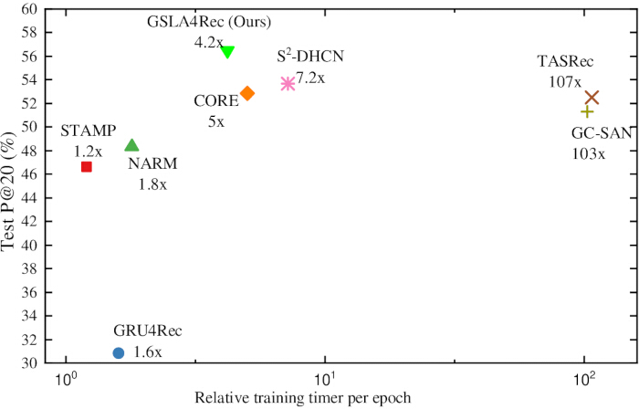
Figure 4: Performance over runtime of GSLA4Rec on Diginetica. The figure showed that our proposed GSLA4Rec and baseline models run on NVIDIA TITAN V GPU using Diginetica for the relative training time per epoch, and GSLA4Rec achieved faster training speed than the baseline models. This figure was self-drawn via OriginPro with fully customized elements. No copyrighted external graphic resources were used, hence no additional third-party copyright licensing was needed. Figure copyright was owned by the authors and would comply with the journal's copyright rules upon acceptance. GSLA4Rec represented gated-slot linear attention graph neural networks for SBR. Please click here to view a larger version of this figure.

To sum up, the efficiency of the proposed GSLA4Rec model with linear-complexity gated-slot attention consistently outperformd SOTA across all datasets. In particular, GSLA4Rec achieved significant performance gains in long-session recommendation scenarios on the Tmall and Nowplaying datasets, and showed superior sequential dependency modeling capability.

Analyzing ablation experiments

Impact of SG and NGG and GSLA

To evaluate the impact of the SG, the NGG, gating mechanism, memory slots and linear attention on the current SBR, ablation studies were performed on the Diginetica, Tmall, and Nowplaying datasets. GSLA4Rec‑NotSG excluded the SG feature encoding while preserving the NGG encoding, GSLA4Rec‑NotNGG discarded the NGG encoding and performed feature extraction solely based on SG, GSLA4Rec‑NotGM removed only the gating mechanism within GSLA, GSLA4Rec‑NotMS eliminated merely the memory slots of GSLA, and GSLA4Rec‑NotLA omited only the linear attention module in GSLA.

Dataset	Diginetica		Tmall		Nowplaying
Measures	P@20	MRR@20	P@20	MRR@20	P@20	MRR@20
GSLA4Recs-NotSG	54.28	18.87	31.40	15.11	22.48	7.45
GSLA4Recs-NotNGG	52.65	17.67	28.90	14.61	20.17	7.74
GSLA4Rec-NotGM	53.82	18.21	39.26	16.52	23.14	7.62
GSLA4Rec-NotMS	53.40	17.60	38.05	15.65	22.55	7.40
GSLA4Rec-NotLA	51.86	16.92	29.12	13.96	20.82	7.28

Table 4: Performance of GSLA4Rec ablation experiments. The table reports the ablation performance of GSLA4Rec after removing individual model components on the Diginetica, Tmall, and Nowplaying datasets, evaluated using P@20 and MRR@20.

Table 4 showed the results of the ablation study on different datasets, all performance metrics decreased compared to the full model. The decrease in performance when removing the near-neighbor global session graph encoding (GSLA4Rec-NotNGG) was stronger than when removing the session graph feature encoding (GSLA4Rec-NotSG). Deleting any submodule in GSLA would result in performance degradation, the performance degradation was ranked from high to low by linear attention, memory slots, and gating mechanism. The reason was that the importance of each item in SBR was definitely different, and there was a need for associative memory between items. It could be seen that GSLA was a key part of this paper's model.

Impact of different aggregation methods

To evaluate the impact of different information aggregation methods on the performance of the GSLA4Rec model, the following three classic information aggregation methods were investigated: 1) Average Pooling: performing an average pooling operation on the vectors generated by the SG and the NGG; 2) Vector Concatenation: concatenating the vectors generated by SG and NGG; 3) Vector Summation: summing the vectors generated by SG and NGG. The results were shown in Table 5. GSLA4Rec with Vec-Sum achieved the best performance on Diginetica, Tmall, and Nowplaying. By contrast, Mean-pooling yielded poor results across all datasets. The inferior performance of mean aggregation and concatenation aggregation might stem from overfitting caused by excessive parameters, which degraded the overall model performance.

Dataset	Diginetica		Tmall		Nowplaying
Measures	P@20	MRR@20	P@20	MRR@20	P@20	MRR@20
Mean-Pooling	45.26	15.63	38.84	16.3	23.56	7.55
Vec-Concating	51.77	17.24	39.83	18.24	24.06	8.88
Vec-Sum	56.47	19.98	43.6	19.96	27.1	9.32

Table 5: Effects of different aggregation methods. The table compares the effects of mean pooling, vector concatenation, and vector summation on GSLA4Rec performance across the Diginetica, Tmall, and Nowplaying datasets using P@20 and MRR@20.

Analyzing hyper-parameter settings

Effects of different memory slot sizes

Memory slots stored information from previous time steps, which was particularly important for tasks with temporal dependencies. This section investigated the impact of memory slot sizes m = [0, 1, 2, 3, 4, 5] on SBR performance. Experimental results, shown in Table 6, indicated that when the memory slots sizes m was set to 3, the metrics P@20 and MRR@20 performed optimally across the three datasets. This suggested that a moderate memory slots sizes effectively improved the model's recommendation accuracy and ranking quality, smaller memory slots struggle to memorize sufficient historical information and focued more on short-term users’ interests, whereas when the memory slots sizes increased to 4 or more, the model stores excessive historical information, causing it to over-rely on historical interests while neglecting more critical current input information, thereby degrading recommendation performance.

Dataset	Diginetica		Tmall		Nowplaying
Measures	P@20	MRR@20	P@20	MRR@20	P@20	MRR@20
GSLA4Rec-m0	53.40	17.60	38.05	15.65	22.55	7.40
GSLA4Rec-m1	55.43	18.92	41.55	17.12	25.60	8.43
GSLA4Rec-m2	56.02	19.35	42.90	18.25	26.62	8.95
GSLA4Rec-m3	56.47	19.98	43.60	19.96	27.10	9.32
GSLA4Rec-m4	53.96	19.25	43.06	19.09	26.34	8.35
GSLA4Rec-m5	52.18	18.03	42.12	17.56	24.86	8.85

Table 6: Effects of different memory slot sizes. The table reports the performance of GSLA4Rec with different memory slot configurations (m0–m5) on the Diginetica, Tmall, and Nowplaying datasets using P@20 and MRR@20.

Effects of different dropout ratios

To prevent overfitting, dropout regularization was introduced. Before summing the session-level item vector and the neighbor global-level item vector, the outputs of neurons were randomly dropped in the neighbor global-level item vector h_i^ngg,(k) to enhance the robustness and generalization ability of the GSLA4Rec model.

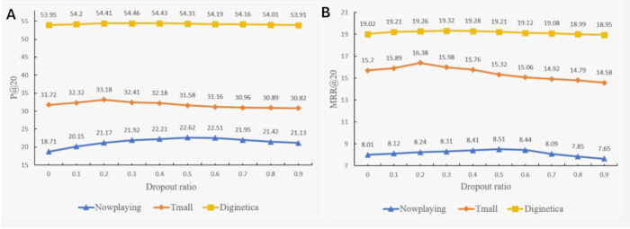
Figure 5: Performance of GSLA4Rec under different dropout ratios. (A) P@20 and (B) MRR@20 of GSLA4Rec under different dropout ratios on the Nowplaying, Tmall, and Diginetica datasets. The performance initially increased and subsequently decreased as the dropout ratio increased, demonstrating the robustness and generalization ability of the model. GSLA4Rec, gated-slot linear attention graph neural networks for session-based recommendation (SBR). This figure was self-drawn using OriginPro with fully customized elements. No copyrighted external graphic resources were used; therefore, no additional third-party copyright licensing was required. Figure copyright was owned by the authors and would comply with the journal's copyright rules upon acceptance. Please click here to view a larger version of this figure.

Figure 5A–B showed the impact of different dropout ratio in Equation (16) on model performance. Experimental results indicated that the model performs poorly when the dropout ratio was low, however, as the dropout ratio increased, model’s performance gradually improved until it reached an optimal level. Specifically, the optimal dropout ratio was 0.3 on the Diginetica dataset, 0.2 on the Tmall dataset, and 0.5 on the Nowplaying dataset. When the dropout ratio exceeded these optimal values, model’s performance began to decline, primarily because excessive neuron dropout prevented the model from effectively learning important features from the session data.

Effects of different embedding size

To minimize computational overhead as much as possible while maintaining optimal model performance, the impact of different embedding dimensions d was investigated on the performance of the GSLA4Rec model. As shown in Figure 6A–B, on three public datasets Diginetica, Tmall, and Nowplaying, the GSLA4Rec model performed poorly when the embedding dimension d was 10–40, however, model’s performance rapidly rose as the value of d increased, the performance metrics tended to stabilize when the value of d was within the range of 80 to 120, then, performance actually declined as d increased continuously possibly due to overfitting caused by a large embedding dimension. Therefore, the dimension of the item embedding vector was finally set to 100.

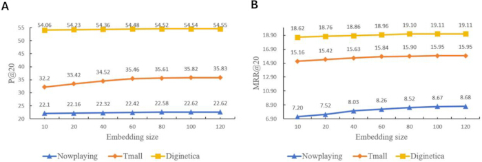
Figure 6: Performance of GSLA4Rec under different embedding sizes. (A) P@20 and (B) MRR@20 of GSLA4Rec under different embedding sizes on the Nowplaying, Tmall, and Diginetica datasets. Model performance progressively increased with increasing embedding size and eventually reached a plateau. GSLA4Rec, gated-slot linear attention graph neural networks for session-based recommendation (SBR). This figure was self-drawn using OriginPro with fully customized elements. No copyrighted external graphic resources were used; therefore, no additional third-party copyright licensing was required. Figure copyright was owned by the authors and would comply with the journal's copyright rules upon acceptance. Please click here to view a larger version of this figure.

Effects of different session lengths

It was well known that the length of each session varies across the three real-world SBR datasets (Diginetica, Tmall, and Nowplaying). To verify the robustness of the GSLA4Rec model compared with baselines on different lengths of sessions, all the sessions in Diginetica and Tmall were divided into three groups, short group (S), medium group (M) and long group (L) respectively from 1 to 6, 7 to 12, greater than 12. MRR@20 was adopted to verify performance of the methods instead of P@20 since the MRR can better reflect the ranking quality of correct results. Figure 7A–B indicated that the GSLA4Rec model outperformed the sequence-based baseline NARM, the GNNs-based baseline SR-GNN, the contrastive learning augmented GNNs baseline S²-DHCN, and the spatio-temporal baseline RESTC with different lengths of sessions. Meanwhile, It was also observed that the performance of all methods decreased with increasing sequence length since long‑range item transitions made it difficult to capture users’ preferences, but the proposed the GSLA4Rec model had the slowest descent speed compared with baselines since Gated-slot mechanism could filter out irrelevant items, the performance of GSLA4Rec respectively surpassed that of the NARM model by 6.3 and 8.85 in the long groups of Diginetica and Tmall.

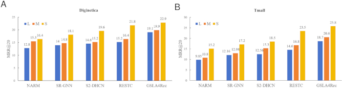
Figure 7: Performance of GSLA4Rec under different session lengths. Performance of GSLA4Rec and baseline models under different session-length groups on the (A) Diginetica and (B) Tmall datasets, evaluated using MRR@20. The session-length groups are denoted as L, M, and S. GSLA4Rec, gated-slot linear attention graph neural networks for session-based recommendation (SBR). This figure was self-drawn using OriginPro with fully customized elements. No copyrighted external graphic resources were used; therefore, no additional third-party copyright licensing was required. Figure copyright was owned by the authors and would comply with the journal's copyright rules upon acceptance. Please click here to view a larger version of this figure.

Conclusion

This paper proposes a global context gated-slot linear attention network for SBR. By combining SG and NGG, and introducing a gated-slot linear attention mechanism, this method enables it to focus on key items in the session sequence, capture long- and short-term dependencies, effectively reduce noise, and decrease computational complexity. Experimental results confirm that this method exhibits excellent recommendation accuracy and efficiency on three public datasets, particularly excelling in long-term dependency modeling tasks.

DATA AVAILABILITY:

Three common public datasets (Diginetica, Tmall, and Nowplaying, URLs can be found in the Table of Materials) that support the findings of this study is openly available on the Internet. At the same time, three widely‑used public datasets and the source code for this work are submitted as Supplementary Folder: GSLA4Rec.zip. Please click here to download this File.

Discussion

Compared with baselines, the GSLA4Rec model achieves dual improvements in performance and efficiency for three core reasons. First, applying gating mechanisms to NGG alleviates data sparsity and filters noise effectively. Second, the memory slots mechanism balances storage capacity and efficiency via hyperparameter m adjustment. Third, the linear attention mechanism computes item correlations at an O(N) complexity, far lower than the O(N²)⁶¹. The GSLA4Rec model overly relies on users' interaction sequences and ignores the multimodal properties of items⁴⁸. Meanwhile, the NGG construction uses a fixed Jaccard threshold without dynamic adjustment function, and the memory slots m cannot achieve adaptive adjustability⁶⁵.

The GSLA4Rec model, which builds SG&NGG and adopts gated-slot linear attention, especially fits anonymous session recommendation³⁹ across e-commerce and online streaming platforms. In e-commerce platforms, this model recommends matching products to users by capturing their browsing, clicking, or adding behaviors to their shopping cart, without relying on user characteristic attributes. The datasets Diginetica and Tmall used in this paper are e-commerce recommendation datasets. For short-video and music streaming platforms, this method analyzes users' playback sequences to infer their implicit preferences, updates content summaries to retain users, and extends viewing time. The dataset Nowplaying used in this paper is the music recommendation dataset.

There are alternative solutions that can replace the gated slot linear attention architecture. The emerging Mamba⁶⁵ based state space model, as an alternative, has the characteristics of selective state storage space and linear computational complexity, balancing linear complexity and long sequence fitting ability, and combined with the LLM⁵⁵ enhancement framework, it extracts the users' implicit intent from the original interaction log, thereby achieving good recommendation performance and efficiency. Future work can optimize GSLA4Rec from multiple perspectives: building dynamic NGG to replace fixed Jaccard filtering, implementing variable memory slots to automatically match sessions of different lengths, and incorporating user multimodal information to improve recommendation accuracy. In addition, with the help of LLM-augmented models⁵⁵, users' implicit intentions can be mined from interaction sequences, and noisy conversation data can be filtered more accurately⁷².

Materials

List of materials used in this article

Name	Company	Catalog Number	Comments
CUDA 11.3	NVIDIA	NONE	CUDA 11.3 is a parallel computing platform and programming model version released by NVIDIA in 2021, aimed at enhancing the performance and development flexibility of GPU accelerated applications.
Diginetica	Diginetica	NONE	Diginetica is the official competition dataset of the 2016 CIKM (International Information Retrieval Conference) Cup, which was used in the CIKM algorithm competition to solve the problem of personalized product retrieval in e-commerce with search context. It has now become the most mainstream standard e-commerce benchmark dataset in the field of Session based Recommendation (SBR).
Nowplaying	Zenodo	NONE	It is a large-scale music listening behavior dataset constructed based on the "# nowplaying" tag tweet mining, with the core used for music conversation recommendation, context aware recommendation, and sentiment correlation analysis research.
OriginPro 2024 (64-bit) SR1	OriginLab Corporation	NONE	OriginPro is a commercial professional scientific drawing and data analysis software developed by OriginLab Corporation, commonly used for drawing paper level charts, data statistics, curve fitting, signal processing, etc. This article uses OriginPro to draw experimental comparison charts, line charts, and bar charts.
PyTorch 1.11.0	PyTorch Foundation	NONE	PyTorch is an open-source deep learning framework for machine learning and deep learning, released by Facebook in 2016. It primarily implements automatic differentiation and introduces dynamic computation graphs to make model building more flexible.
TITAN V GPU	NVIDIA	NONE	NVIDIA TITAN V is a flagship graphics card launched by NVIDIA at the end of 2017, mainly aimed at high-performance computing and artificial intelligence fields.
Tmall	Tmall	NONE	From IJCAI 2015 Alibaba Tmall Recommendation Competition, Alibaba Tianchi publicly released desensitized real Tmall online logs. It is one of the three standard datasets in the SBR field (Diginetica, Yoocoose, Tmall) and the preferred evaluation set for Chinese e-commerce scenarios.
visio 2021	Microsoft	NONE	Visio is a vector drawing software developed by Microsoft, used  to draw model structure diagrams, flowcharts, framework diagrams, network topology diagrams in scientific research papers, and output vector diagrams for paper illustrations

References

- Sarwar B, Karypis G, Konstan J, Riedl J. Item-based collaborative filtering recommendation algorithms. In: Proceedings of the 10th International Conference on World Wide Web; 2001 May 1–5; Hong Kong, China. ACM; 2001.p.285-295.
- Zhao ZD, Shang MS. User-based collaborative-filtering recommendation algorithms on hadoop. In: 2010 Third International Conference on Knowledge Discovery and Data Mining; 2010 Jan 9–10; Washington, DC, USA. IEEE; 2010.p.478-481.
- Koren Y, Rendle S, Bell R. Recommender Systems Handbook. Berlin: Springer; 2022.
- Koren Y, Bell R, Volinsky C. Matrix factorization techniques for recommender systems. Computer. 2009;42(8):30-37.
- Rendle S, Freudenthaler C, Schmidt-Thieme L. Factorizing personalized markov chains for next-basket recommendation. In: Proceedings of the 19th International Conference on World Wide Web; 2010 Apr 26–30; Raleigh, North Carolina, USA. ACM; 2010.p.811-820.
- Wang S et al. A survey on session-based recommender systems. ACM Comput Surv. 2021; 54(7): 1-38.
- Ninichuk M, Namiot D. Survey On Methods For Building Session-Based Recommender Systems. Int J Open Inf Technol. 2023;11(5):22-32.
- Saxena A. A Survey of Session-Based Recommender Systems. In: 2023 5th International Conference on Advances in Computing, Communication Control and Networking. IEEE, 2023.
- Ravanmehr R, Mohamadrezaei R. Session-Based Recommender Systems Using Deep Learning. Berlin: Springer; 2023.
- He R, McAuley J. Fusing similarity models with markov chains for sparse sequential recommendation. In: 2016 IEEE 16th International Conference on Data Mining; 2016 Dec 12–15; Barcelona, Spain. IEEE; 2016.p.191-200.
- Chen R, Fan J, Wu M. MC-RGN: Residual graph neural networks based on Markov chain for sequential recommendation. Inf Process Manag. 2023;60(6):103519.
- Ni S, Hu S, Li L. An intention-aware markov chain based method for top-k recommendation. IEEE Trans Autom Sci Eng. 2022;21(1):581-592.
- Yu Y, Si X, Hu C, Zhang J. A review of recurrent neural networks: LSTM cells and network architectures. Neural Comput. 2019;31(7):1235-1270.
- Mienye ID, Swart TG, Obaido G. Recurrent neural networks: A comprehensive review of architectures, variants, and applications. Information. 2024;15(9):517.
- Hidasi B, Karatzoglou A, Baltrunas L, Tikk D. Session-based recommendations with recurrent neural networks. In: Bengio Y, LeCun Y, editors. Proceedings of International Conference on Learning Representations; 2016 May 2–4; San Juan, Puerto Rico.
- Li J et al. Neural attentive session-based recommendation. In: Proceedings of the 2017 ACM Conference on Information and Knowledge Management; 2017 Nov 6–10; Singapore. ACM; 2017. p.1419-1428.
- Liu Q, Zeng Y, Mokhosi R, Zhang H. STAMP: short-term attention/memory priority model for session-based recommendation. In: Proceedings of the 24th ACM SIGKDD International Conference on Knowledge Discovery & Data Mining; 2018 Aug 19–23; London, United Kingdom. ACM; 2018.p.1831-1839.
- Zhou J et al. Graph neural networks: A review of methods and applications. AI open. 2020;1:57-81.
- Scarselli F, Gori M, Tsoi AC, Hagenbuchner M, Monfardini G. The graph neural network model. IEEE Trans Neural Netw. 2009;20(1):61‑80.
- Corso G, Stark H, Jegelka S, Jaakkola T, Barzilay R. Graph neural networks. Nat Rev Methods Primers. 2024;4(1):17.
- Zheng Y, Yi L, Wei Z. A survey of dynamic graph neural networks. Front Comput Sci. 2025;19(6):196323.
- Wu S et al. Session-based recommendation with graph neural networks. In: Proceedings of the AAAI Conference on Artificial Intelligence; 2019 Jan 27‑Feb 1; Honolulu, USA. AAAI Press; 2019.p.346-353.
- Wang Z et al. Global context enhanced graph neural networks for session‑based recommendation. In: Proceedings of the 43rd International ACM SIGIR Conference on Research and Development in Information Retrieval; 2020 Jul 25‑30; Virtual conference. ACM; 2020.p.169‑178.
- Shani G, Heckerman D, Brafman RI. An MDP‑based recommender system. J Mach Learn Res. 2005;6:1265‑1295.
- Gu W, Dong S, Zeng Z. Increasing recommended effectiveness with Markov chains and purchase intervals. Neural Comput Appl. 2014;25(5):1153‑1162.
- O'shea K, Nash R. An introduction to convolutional neural networks. arXiv preprint arXiv:1511.08458, 2015.
- Wu J. Introduction to convolutional neural networks. Nanjing: National Key Lab for Novel Software Technology, Nanjing University; 2017.
- Li Z, Yang W, Peng S, Liu F. A survey of convolutional neural networks: analysis, applications, and prospects. IEEE Trans Neural Netw Learn Syst. 2021;33(12):6999‑7019.
- Krichen M. Convolutional neural networks: A survey. Computers. 2023;12(8):151.
- Tang J, Wang K. Personalized top-n sequential recommendation via convolutional sequence embedding. In: Proceedings of the 11th ACM International Conference on Web Search and Data Mining; 2018 Feb 5–9; Marina Del Rey, California, USA. ACM; 2018.p.565-573.
- Tuan T, Phuong T. 3D convolutional networks for session-based recommendation with content features. In: Proceedings of the 11th ACM Conference on Recommender Systems; 2017 Aug 27–31; Como, Italy. ACM; 2017.p.138-146.
- Graves A. Generating sequences with recurrent neural networks. arxiv preprint arxiv: 1308.0850, 2013.
- Tang D, Qin B, Liu T. Document modeling with gated recurrent neural network for sentiment classification. In: Proceedings of the 2015 Conference on Empirical Methods in Natural Language Processing; 2015 Sep 17‑21; Lisbon, Portugal. Association for Computational Linguistics; 2015.p.1422‑1432.
- Chan W, Jaitly N, Le Q, Vinyals O. Listen, attend and spell: a neural network for large vocabulary conversational speech recognition. In: 2016 IEEE International Conference on Acoustics, Speech and Signal Processing; 2016 Mar 20‑25; Shanghai, China. IEEE; 2016.p. 4960‑4964.
- Sutskever I, Vinyals O, Le QV. Sequence to sequence learning with neural networks. In: Advances in Neural Information Processing Systems 27; 2014 Dec 8‑13; Montreal, Canada.
- Xiao C, Li Z, Tang J, Lee J. United prediction of travel modes and purposes in travel chains based on multitask learning deep neural networks. Mathematics. 2025;13(9):1528.
- Chmielewski J, Wójcik M. The use of deep neural networks (DNN) in travel demand modelling. Appl Sci. 2025;15(20):11290.
- Shahmoradi N, Alesheikh AA, Jafari A, Lotfata A. Hybrid ST-ResNet and LSTM approach for precise crime hotspot prediction. Sci Rep. 2025;15:18672.
- Park J, Yi D, Ji SM. Analysis of recurrent neural network and predictions. Symmetry.2020;12(4): 615.
- Ramakrishnan N, Soni T. Network traffic prediction using recurrent neural networks. In: 2018 17th IEEE International Conference on Machine Learning and Applications; 2018 Dec 17‑20; Orlando, Florida, USA. IEEE; 2018.p.187‑193.
- Yu P, Yan X. Stock price prediction based on deep neural networks. Neural Comput Appl. 2020;32(6):1609‑1628.
- Zhao J, Zeng D, Liang S, Kang H, Liu Q. Prediction model for stock price trend based on recurrent neural network. J Ambient Intell Humaniz Comput. 2021;12:745‑753.
- Zaytar MA, Chaker EA. Sequence to sequence weather forecasting with long short-term memory recurrent neural networks. Int J Comput Appl. 2016;143(11):7-11.
- Xu L, Peng J, Jiang X, Chen E, Luo B. Graph neural network based on graph kernel: a survey. Pattern Recognit. 2025;161:111307.
- Li Y, Tarlow D, Brockschmidt M, Zemel R. Gated graph sequence neural networks. arxiv preprint arxiv: 1511.05493, 2015.
- Kipf TN, Welling M. Semi-supervised classification with graph convolutional networks. arXiv preprint arXiv:1609.02907;2016.
- Veličković P et al. Graph attention networks. arXiv preprint arXiv:1710.10903;2017.
- Chen L, Zhu X, Zhu G. Exploiting attributes and keywords for session-based recommendation with multi-view graph neural network. Expert Syst Appl. 2025;128990.
- Driss El Alaoui et al. A novel session-based recommendation system using capsule graph neural network. Neural Netw. 2025;185:107176.
- Xu C et al. Graph contextualized self‑attention network for session‑based recommendation. In: Proceedings of the 28th International Joint Conference on Artificial Intelligence; 2019 Aug 10‑16; Macao, China. 2019.p.3940‑3946.
- Qiu R, Huang Z, Li J, Chen H. Rethinking the item order in session‑based recommendation with graph neural networks. In: Proceedings of the 28th ACM International Conference on Information and Knowledge Management; 2019 Nov 3‑7; Beijing, China. ACM; 2019.p.579‑588.
- Chen J, Ji J, Li H, Zhang X. SR‑HetGNN: session‑based recommendation with heterogeneous graph neural network. Knowl Inf Syst. 2024;66(2):1111‑1134.
- Wang Y et al. Knowledge graph‑based session recommendation with session‑adaptive propagation. In: Companion Proceedings of the ACM Web Conference 2024; 2024 May 13‑17; Singapore. ACM; 2024.p.264‑273.
- Wang Z, Jin B. DiffSBR: a diffusion model for session-based recommendation. Inf. Process. Manag. 2026;63(1):104284.
- Qiao S et al. Multi-view intent learning and alignment with large language models for session-based recommendation. ACM Trans. Inf. Syst. 2025;43(4):91.
- Wang M et al. A collaborative session‑based recommendation approach with parallel memory modules. In: Proceedings of the 42nd International ACM SIGIR Conference on Research and Development in Information Retrieval; 2019 Jul 21‑25; Paris, France. ACM; 2019. p.345‑354.
- Ye R, Zhang Q, Luo H. Cross-session aware temporal convolutional network for session-based recommendation. In: 2020 International Conference on Data Mining Workshops; 2020 Nov 16–19; Sorrento, Italy. IEEE Computer Society; 2020.p.220-226.
- Chen Y, Huang L, Wang C, Lai J. Hybrid-order gated graph neural network for session-based recommendation. IEEE Trans Ind Inform. 2021;18(3):1458‑1467.
- Chen Y, Tang Y, Yuan Y. Attention-enhanced graph neural networks with global context for session-based recommendation. IEEE Access. 2023;11:26237-26246.
- Tang L, Wang X, Wang H, Shi C, Song L. DA‑GCN: a domain‑aware attentive graph convolution network for shared‑account cross‑domain sequential recommendation. In: Proceedings of the 30th International Joint Conference on Artificial Intelligence; 2021 Aug 19‑27; Montreal, Canada.
- Vaswani A et al. Attention is all you need. In: Advances in Neural Information Processing Systems 30; 2017 Dec 4‑9; Long Beach, USA.
- Lu Y, Letey M, Zavatone‑Veth JA, Maiti A, Pehlevan C. Asymptotic theory of in‑context learning by linear attention. Proc. Natl. Acad. Sci. U.S.A. 2025;122(28):e2502599122.
- Peng H, Pappas N, Yogatama D, Kong L. ABC: attention with bounded‑memory control. In: Proceedings of the 60th Annual Meeting of the Association for Computational Linguistics; 2022 May 22‑27; Dublin, Ireland. Association for Computational Linguistics; 2022.p.7469‑7483.
- Yang S et al. Gated linear attention transformers with hardware‑efficient training. In: Proceedings of the 41st International Conference on Machine Learning; 2024 Jul 21‑27; Vienna, Austria. PMLR; 2024.
- Yuan H et al. DG‑mamba: robust and efficient dynamic graph structure learning with selective state space models. In: Proceedings of the 39th AAAI Conference on Artificial Intelligence; 2025 Feb 25‑Mar 4; Philadelphia, Pennsylvania, USA. AAAI Press; 2025.p.22272‑22280.
- Xia X et al. Self‑supervised graph co‑training for session‑based recommendation. In: Proceedings of the 30th ACM International Conference on Information and Knowledge Management; 2021 Oct 25‑29; Virtual Event. ACM; 2021.p.2180‑2190.
- Zhou H, Zhang D, Song M, Han W. Temporal augmented graph neural networks for session‑based recommendations. In: Proceedings of the 44th International ACM SIGIR Conference on Research and Development in Information Retrieval; 2021 Jul 11‑15; Montreal, Canada. ACM; 2021. p. 1798‑1802.
- Chen Q, Jiang F, Wang Y, Li Y, Zhang Y. Combine temporal information in session‑based recommendation with graph neural networks. Expert Syst Appl. 2024;238:121969.
- Hou Y, Hu B, Zhang Z, Zhao W. Core: simple and effective session‑based recommendation within consistent representation space. In: Proceedings of the 45th International ACM SIGIR Conference on Research and Development in Information Retrieval; 2022 Jul 11‑15; Madrid, Spain. ACM; 2022.p.1796‑1801.
- Wan Z et al. Spatio‑temporal contrastive learning‑enhanced GNNs for session‑based recommendation. ACM Trans. Inf. Syst. 2023;42(2):1‑26.
- Zeng X et al. RAIN: reconstructed‑aware in‑context enhancement with graph denoising for session‑based recommendation. Neural Netw. 2025;184:107056.
- Zhan H et al. Capturing dynamic interests with deformable attention mechanism for session-based recommendation. Int J Mach Learn Cybern. 2026;17:375.