Optimized Methods of Investigating Developmental Protein and Transcript Expression in Whole-mount Mouse Embryos

Summary

Mouse models are instrumental in advancing our understanding of embryonic development. Here, we describe a protocol to stain proteins and transcripts in whole-fixed mouse embryos, and how to quantitatively analyze the resulting staining in three dimensions. These techniques allow visualization and analysis of key developmental cell types and processes.

Abstract

Mouse models have been instrumental in advancing our understanding of embryonic development. Analyzing the expression and localization of proteins and transcripts within embryos is critical for elucidating cellular and molecular mechanisms underlying development and disease. However, traditional techniques used to analyze transcripts and proteins in mouse embryos are limited. RNA in situ hybridization permits whole-mount staining of transcripts but lacks multiplexing capability. By contrast, sectioning of embryos allows for multiplexed target staining, but only in two-dimensions (2D). More recently, techniques such as RNAscope and immunofluorescence staining have been applied to whole-mount embryos, allowing multiplexing of targets in three-dimensions (3D). These methods enable mapping of key interactions, pathways, and cell types necessary for embryonic development without the limitations of traditional techniques.

Here we describe optimized methods for whole-mount staining of fixed embryonic day (E) 8.5 and E9.5 mouse embryos using either RNAscope or immunofluorescence. Both enable multiplexed detection of up to 4 targets simultaneously in a single embryo. We also provide a method to combine immunofluorescence staining with RNAscope in the same embryo to visualize the interplay between proteins and transcripts during development. Furthermore, we describe a pipeline of confocal imaging and 3D analysis of target expression across the whole embryo and within defined developmental cell types using Zeiss Arivis Pro software. Together, these methods allow comprehensive analysis of multiplexed protein and transcript targets in 3D, providing a powerful system for dissecting cellular and molecular interactions in early to mid-embryogenesis.

Introduction

Mouse models have been instrumental for advancing progress in developmental biology, by allowing the understanding of human-relevant developmental processes in vivo due to the homology between mouse and human development and the ability to modulate gene expression by use of key techniques such as Cre-LoxP or CRISPR/Cas9^1,2. Around 90% of genomic regions are conserved between mice and humans³, and mice and humans share many developmental processes. For example, both mice and humans follow a similar timeline of embryogenesis, including the formation of a zygote that progresses to a blastocyst, followed by implantation and gastrulation⁴. Furthermore, the development of most organs is similar between mice and humans. For example, both the human and mouse heart follow a similar sequence of cardiac looping, septation of the atria and ventricles, valve formation, and outflow tract formation to form a four-chambered heart⁵. Thus, both developing and fully developed mouse and human hearts have significant structural similarity^6,7.

In order to investigate the processes that occur in normal and pathological development, multiple techniques have been developed, allowing for the visualization of key proteins and transcripts spatially. Such techniques include immunofluorescence staining and RNA in situ hybridization.

RNA in situ hybridization was first described by Gall and Pardue⁸ and John, Brinstall, and Jones, in 1969⁹, and Buongiorno-Nardelli and Amaldi¹⁰ in 1970. It is used to look at transcript expression in tissue⁸. Briefly, probes containing a complementary sequence of RNA to the desired target are selected and labeled with markers for detection. Such labels include radioactive labels, biotin, or digoxigenin. Fixed samples are permeabilized to allow probe penetration, and then the probe is hybridized to the tissue. Tissues can then either be directly imaged if radioactively labeled, or labels visualized using antibodies conjugated to alkaline phosphatase or a fluorescent dye. RNA in situ hybridization has the benefit of being able to stain whole-mount samples for 3D localization¹¹. However, it is usually limited by its lack of multiplexing capacity of greater than 2 targets, unless optimized techniques with very specific applications are used, or DNA hybridization is used, such as M-FISH, which is used for fluorescent labeling of chromosomes^12,13.

Immunofluorescence, first developed in 1941 by Coons et al.^14,15, is a method of target protein detection in fixed or frozen samples. Briefly, samples are blocked to reduce non-specific binding to non-target areas of tissue. Then, a primary antibody specific to a target antigen is incubated with the samples. Primary antibodies can be directly conjugated to a fluorescent dye or protein or can be themselves targeted using a fluorescently conjugated secondary antibody targeting the species in which the primary antibody was raised. The benefit of using secondary antibodies over directly conjugated primary antibodies is that the signal is amplified, leading to greater sensitivity. Multiple primary antibodies raised in different species can be used to multiplex target detection, using directly conjugated or secondary antibodies conjugated to fluorophores with different excitation and emission spectra.

Traditional techniques such as RNA in situ hybridization and immunofluorescence are limited. Typically, RNA in situ hybridization only allows for the detection of a single target in a sample, so interaction between different cell types and pathways is extremely limited. Furthermore, immunofluorescence is traditionally performed in tissue sections rather than in whole-mount, limiting spatial resolution to 2D. More recent techniques have focused on multiplexing target detection in 3D systems. Optimization of immunofluorescence protocols has allowed for the use of the technique in whole-mount¹⁶. Furthermore, techniques have been developed to be able to multiplex transcript detection by using fluorescently labeled probes, in a similar manner to immunofluorescence.

RNAscope was first described in 2012 by Wang et al. It is based on RNA in situ hybridization technology¹⁷, which allows for spatial identification of transcripts in fixed samples. Briefly, fixed samples are permeabilized, allowing for infiltration of target probes that bind to complementary transcript sequences. RNAscope probes have a ‘double-Z design’ consisting of a region that is specific to an 18–25 base pair region of target RNA, a tail region containing 14 base pairs, and a spacer region that links two ‘Z probes’ together. The two tail regions together form a 28bp region that is bound by a pre-amplifier. Bound Z probe pairs are then amplified through the binding of a sequence of amplifiers that bind to sites on the pre-amplifier. Amplifiers can be specifically targeted using labelled probes tagged with fluorescent markers or horseradish peroxidase (HRP). The idea of the double Z design of the probes is to prevent amplification of unbound probes, reducing non-specific amplification, whereas the use of multiple amplifiers is to enhance sensitivity. The benefit of RNAscope over RNA in situ hybridization is the ability to multiplex transcript detection in a single sample by the use of distinct fluorescent markers for each target. RNAscope has been widely used in formalin-fixed paraffin-embedded sections of samples, allowing spatial transcript detection in 2D¹⁸. More recent studies have described whole-mount RNAscope staining in mouse embryos, allowing 3D analysis of key developmental processes¹⁹.

Here, we describe optimized methods of staining fixed E8.5 and E9.5 mouse embryos in whole-mount using both RNAscope in situ hybridization and immunofluorescence. This protocol describes a revised method of combining immunofluorescence and RNAscope that is successful for whole-mount E8.5/E9.5 embryos, allows for adding a further channel to whole-mount RNAscope staining by incorporating staining using a fourth RNAscope probe combined with the Opal 780 fluorophore, and details a widely applicable method for analysis of stained embryos. These methods can be used to further advance knowledge of key developmental processes such as cell migration and signaling pathways by allowing multiplexed visualization of up to 4 protein and transcript targets by immunofluorescence staining and RNAscope, and quantitative 3D analysis in wholemount E8.5/E9.5 mouse embryos during development.

Protocol

All animal experiments were performed in compliance with the UK Animals (Scientific Procedures) Act 1986 and approved by the University of Oxford animal welfare review board and the Home Office (Project license PP7967396).

1. Dissection, dehydration, and storage of E8.5 and E9.5 mouse embryos

1. Cull pregnant females using an approved method at E8.5 or E9.5 gestation.
   NOTE: Mice in this study were culled using cervical dislocation followed by confirmation of death by exsanguination. Exsanguination is performed by making an incision in the ventricles, facilitating bleeding. Other methods, such as CO2 inhalation, may be used, but were not tested in this protocol.
2. Open the abdomen first by cutting through the skin, then the abdominal wall.
   NOTE: Swab mice with 70% ethanol to reduce dander and bacterial contamination. When opening the abdominal wall, it is important to pull the wall away from the abdomen, then make a small incision. Cut the abdominal wall in a V-shape, avoiding inadvertently cutting the uterus.
3. Remove the uterus by cutting where the uterus meets the vagina. For both uterine horns, cut the uterus away from the abdominal fat, making small excisions until you reach the ovary.
   NOTE: It is worthwhile to make a note of the position of each embryo within the uterus. Dissect out the ovary with the uterus to help maintain orientation.
4. Individually cut a single embryo from the uterine horn, within the surrounding uterus, and place it in a dish containing 1× Hanks’ Basic Salt Solution with 5mM EDTA.
5. Using fine forceps, gently peel away the uterus from the embryo, placenta, and the decidua surrounding the two.
6. Identify where the placenta meets the part of the maternal decidua surrounding the embryo; there should be a slight difference in color between these two sections. Carefully separate the embryo by cutting through the maternal decidua to disconnect the placenta and reveal the embryo.
7. Gently tease the embryo within its yolk sac from the remaining tissue. Using fine forceps, remove the yolk sac surrounding the embryo. Remove the amnion. Count somites to determine the exact embryonic stage.
   NOTE: The yolk sac surrounds the embryo and is thicker and more opaque. The amnion is thin, transparent, and clings tightly to the embryo. This needs to be carefully removed to ensure downstream probe/antibody penetration. For older embryos, a hole can be poked in the head with fine forceps to prevent probe trapping in the developing brain ventricles. It is important at this point to remove as much of the yolk sac as possible. Leftover yolk sac fluoresces strongly when anti-mouse secondary antibodies are used.
8. Optional: Store the yolk sac for genotyping by washing in 500 µL of PBS or 70% ethanol, depending on downstream genotyping, in a 1.5 mL Eppendorf tube to remove contaminating blood. Hold the yolk sac in the PBS using fine forceps and manually agitate. Take the washed yolk sac and place it in a clean 1.5 mL Eppendorf tube or genotyping plate. Store for up to 4 weeks at -20 °C or proceed to the preferred DNA extraction technique.
9. Using a 2 mL low-density polyethylene (LDPE) Pasteur pipette, gently pipette the embryo and move to a 2 mL round-bottomed Eppendorf containing 1 mL of freshly made or frozen stock 4% paraformaldehyde (PFA), taking care to add minimal dissection media to the PFA.
   NOTE: When dissecting E9.5 embryos, cut the end of the Pasteur pipette at an angle to increase the size of the opening. This is important to avoid damage to the embryo when pipetting. Use of round-bottomed 2 mL Eppendorf tubes is important to prevent the embryo from getting stuck in the bottom of the tube and allowing easier recovery. Avoid repeated freeze-thaw cycles of PFA.
   CAUTION: PFA is toxic and carcinogenic. Use appropriate personal protective equipment (PPE) and do not inhale or ingest. Powdered PFA is dangerous if inhaled; therefore, it must be prepared in a fume hood.
10. Incubate the embryo in 4% PFA for 16–24 h at 4 °C with gentle rocking, with tubes at right angles to the direction of rocking.
11. Dehydrate the embryo using washes in a methanol series. Using LDPE Pasteur pipettes and taking care not to pipette up the embryo, take off PFA and add 1 mL PBS. Wash for 10 min at room temperature (RT) with gentle rocking, with tubes at 90° to the plane of rocking. Repeat for washes in 25%, 50% 75% and 2× 100% methanol in PBS.
12. Replace the last 100% methanol wash with 1.5 mL of fresh 100% methanol and store at -20 °C.
    NOTE: Samples can be stored for years at -20 °C. Take care to avoid evaporation.
    CAUTION: Methanol is flammable and toxic. Wear appropriate PPE and store in a flammables cabinet. Do not inhale or ingest.

2. Staining whole-mount E8.5 and E9.5 embryos for proteins using immunofluorescence

NOTE: All wash steps are 1 mL volume performed in a 2 mL round-bottomed Eppendorf tube. Perform 1mL wash steps with gentle rocking and tubes at 90° to the plane of rocking. Remove and replace liquid using a 2 mL LDPE Pasteur pipette, taking care not to pipette up the embryo. When using E9.5 embryos, cut the end of the Pasteur pipette to prevent damage to the embryo in the case of inadvertent pipetting. Dilute methanol in PBS. Embryos can be stained individually or in a tube with up to 12 pooled embryos. For E9.5 embryos: up to 2 conditions can be stained in a single tube. If using multiple conditions, cut the tail of one of the groups so they can be distinguished when imaging.

1. Retrieve embryos from -20 °C storage and allow them to come to room temperature (RT) at 20–26 °C for 10–20 min. Make sure embryos have similar somite numbers to ensure comparison of similar developmental stages.
2. Bleach and permeabilize the embryos in a solution of 100% methanol: Dimethyl sulfoxide (DMSO):30% hydrogen peroxide in a 4:1:1 ratio for 2 h.
   CAUTION: Hydrogen peroxide is corrosive and irritant. It can cause serious eye damage and be harmful if swallowed. If hydrogen peroxide is in the eye, rinse with water for several minutes. Hydrogen peroxide is an aquatic hazard; dispose of it at an approved waste disposal facility. Wear appropriate PPE, including eye protection. Do not ingest.
3. Pre-heat the heat block to 98 °C, prepare the citrate unmasking buffer by diluting 100 µL of citrate unmasking buffer in 10.7 mL of distilled water.
4. Rehydrate the samples by rinsing in 70% methanol, then washing in 50% methanol, 25% methanol, then PBS for 10 min each at RT with rocking.
5. Preheat citrate unmasking buffer to 98 °C using the pre-heated heat block for at least 20 minutes. Wash the embryos in citrate unmasking buffer for 3 x 10 min at RT.
6. After RT washes, add pre-heated citrate unmasking buffer to the embryos and heat in the heat block at 98 °C for 10 min. Remove from heat and allow to cool for at least 40 min.
   NOTE: Do not use citrate unmasking buffer for antigen retrieval in E8.5 embryos, as it can lead to embryo dissociation. Embryos can become sticky when in citrate unmasking buffer, so keep the washes stationary to avoid embryo damage due to clumping.
7. Wash the embryos for 3 × 10 min in PBS + 0.1% Triton-X at RT with rocking. Block embryos for 16–24 h in a minimum of 150 µL/tube PBS + 0.1% Triton-X + 10% normal donkey serum at 4 °C with rocking.
8. Prepare the primary antibodies by diluting them in PBS + 0.1% Triton-X + 10% normal donkey serum in recommended concentrations 1 h before placing on embryos and keep at 4 °C.
9. Remove the blocking solution from the embryos and add a minimum of 150 µL/tube of the diluted antibody solution. Incubate for 1–3 days at 4 °C with rocking.
   NOTE: Primary antibodies can be multiplexed as long as each antibody is raised in a different species. Use of antibodies raised in mice, and subsequent anti-mouse secondary antibodies, can lead to bright non-specific staining. Alternatively, in some instances, primary antibodies of a single species can be multiplexed, where primary antibodies are of a different isotype and combined with isotype-specific secondary antibodies.
10. Rinse embryos in PBS + 0.1% Triton-X, wash embryos for 6 × 30 min in PBS + 0.1% Triton-X at RT.
11. Block secondary antibody by diluting appropriate fluorescently conjugated secondary antibodies and DAPI (or alternative nuclei marker) in 0.1% Triton-X + 10% normal donkey serum in recommended concentrations 1 h before placing on embryos at 4 °C in the dark.
12. Remove wash and add diluted secondary antibody solution to the embryos and incubate for 16–24 h at 4 °C with rocking in the dark.
    NOTE: We recommend using F(ab) fragment fluorescently conjugated secondary antibodies rather than whole antibodies. F(ab) fragments are smaller, therefore have better tissue penetration, and the lack of the Fc region helps to reduce non-specific background.
13. Rinse embryos in PBS + 0.1% Triton-X, then wash embryos for 6 × 30 min in PBS + 0.1% Triton-X at RT with rocking in the dark. Store for up to 4 weeks in PBS + 0.1% Triton-X at 4 °C in the dark.

3. Staining whole-mount E8.5 and E9.5 embryos for transcripts using RNAscope

NOTE: All wash steps are 1 mL in volume, performed in a 2 mL Eppendorf tube. Perform 1 mL wash steps with gentle rocking and tubes at 90° to the plane of rocking. Remove and replace liquid using a 2 mL LDPE Pasteur pipette, taking care not to pipette up the embryo. When using E9.5 embryos, cut the end of the Pasteur pipette to prevent damage to the embryo in the case of inadvertent pipetting. Methanol should be diluted with PBS. Switch on the hybridization oven prior to starting at 40 °C with some damp tissue at the bottom. Embryos can be stained individually or in a tube with up to 12 pooled embryos. For E9.5 embryos: up to 2 conditions can be stained in a single tube. If using multiple conditions, cut the tail of one of the groups so they can be distinguished when imaging.

1. Prepare the bench, pipettes, and rack by cleaning with 70% ethanol followed by an RNase decontamination solution.
2. Rehydrate embryos through a graded methanol series diluted in PBS of 75%, 50%, 25%, PBS, and PBS + 0.1% Tween 20, for 5 min per step with gentle rocking.
3. Permeabilize embryos by incubating in ~75 µL (3 drops) of protease III for 20 min at RT with upright rocking.
   NOTE: Permeabilization time can be optimized by embryonic stage/size. 20 min works well for E8.5/E9.5 embryos, but longer incubations might be needed to see deeper structures in E9.5 embryos. Too long permeabilization steps can lead to embryo dissociation.
4. Wash embryos in PBS + 0.01% Tween 20 for 3 × 5 min.
5. Prepare RNAscope probes by putting approximately 150 µL (around 6 drops) per tube of C1 probes into an Eppendorf tube. Dilute any C2–C4 probes in the C1 probe at a concentration of 1:50 and incubate upright in a hybridization oven at 40 °C for 10 min prior to placing on embryos.
   NOTE: For each set of RNAscope probes in an experiment, ‘C’ indicates the channel designation. A C1 probe is needed, as all other probes are diluted in the C1 probe. Make sure only one probe of each channel designation is used in each mix. Probe mixes can be reused at least 1× if stored at 4 °C for up to 6 weeks.
6. Remove the last wash and add 150 µL of probe mix to each tube of embryos. Incubate in a hybridization oven upright for 16–24 h at 40 °C.
7. Remove probe mix and wash in 0.2× Saline-Sodium Citrate (SSC) buffer + 0.1% Tween 20 for 3 × 8 min at RT.
8. Post-fix embryos in 4% PFA at RT with gentle rocking, with tubes at 90° to the plane of rocking.
9. Wash in 0.2× SSC buffer + 0.1% Tween 20 for 3 × 8 min at RT.
10. Incubate samples in approximately 150 µL (6 drops)/tube of Amp1 reagent for 30 min at 40 °C in a hybridization oven, keeping tubes upright.
11. Wash in 0.2× SSC buffer + 0.1% Tween 20 for 3 × 8 min at RT.
12. Incubate samples in approximately 150 µL (6 drops)/tube of Amp2 reagent for 30 min at 40 °C in a hybridization oven, keeping tubes upright.
13. Wash in 0.2× SSC buffer + 0.1% Tween 20 for 3 × 8 min at RT.
14. Incubate samples in approximately 150 µL (6 drops)/tube of Amp3 reagent for 15 min at 40 °C in a hybridization oven, keeping tubes upright.
15. Wash in 0.2× SSC buffer + 0.1% Tween 20 for 3 × 8 min at RT.
16. Incubate in 150 µL (6 drops) HRP-C1 for 15 min at 40 °C upright in a hybridization oven. Wash in 0.2× SSC buffer + 0.1% Tween 20 for 3 × 8 min at RT.
17. Incubate samples with a fluorophore diluted in TSA buffer for 30 min at 40 °C in a hybridization oven, keeping tubes upright.
    NOTE: RNAscope fluorophores can be used on different probes. TSA-vivid 570 is the brightest, then TSA-vivid 650, then TSA-vivid 520. Select fluorophores based on expected probe abundance.
18. Wash in 0.2× SSC buffer + 0.1% Tween 20 for 3 × 8 min at RT.
19. In the dark, incubate samples in approximately 150 µL (6 drops)/tube of HRP-blocker reagent for 15 min at 40 °C in a hybridization oven, keeping tubes upright.
20. Wash in 0.2× SSC buffer + 0.1% Tween 20 for 3 × 8 min at RT.
    NOTE: The protocol can be paused here for 16–24 h by leaving the embryos in the last wash at RT.
21. Repeat steps 3.16–3.20 for each of probes C2–C4 if being used, swapping HRP-C1 for HRP C2/C3/C4 as required. Use a different fluorophore for each separate probe.
    NOTE: If using C4 probes, the RNAscope 4-plex ancillary kit and the Opal 780 fluorophore are required. Opal 780 should only be used when multiplexing of 4-probes is needed and should be the last fluorophore used, as it is sensitive to degradation. When selecting fluorophores, it is important to consider the capabilities of the microscopy platform you will be using. Always check that the imaging system has appropriate excitation wavelengths, emission filtering, and detector sensitivity for all probes used. When staining with Opal 780, replace steps 3.17–3.19 with the following:
    1. Incubate samples in 150 µL/tube TSA-DIG (diluted 1:100 in TSA-buffer) for 30 min at RT with gentle rocking.
    2. Wash in 0.2× SSC buffer + 0.1% Tween 20 for 3 × 8 min at RT.
    3. In the dark, incubate samples in approximately 150 µL (6 drops)/tube of HRP-blocker reagent for 15 min at 40° in a hybridization oven, keeping tubes upright.
    4. Wash in 0.2× SSC buffer + 0.1% Tween 20 for 3 × 8 min at RT.
    5. Incubate samples in 150 µL/tube of Opal Polaris 780 diluted in Antibody Diluent/Block for 45 min at 40 °C in a hybridization oven, keeping tubes upright
22. In the dark, incubate samples in approximately 150 µL of DAPI diluted in 0.2 x SSC buffer + 0.1% Tween 20 (working concentration 1µg/mL) for 16–24 h at 4 °C with gentle rocking, keeping tubes upright
23. Wash in 0.2× SSC buffer + 0.1% Tween 20 for 3 × 8 min at RT. Store samples short-term in PBS at 4 °C.

4. Combined RNAscope and immunofluorescence staining in whole-mount E8.5 embryos

1. Follow steps 3.1–3.21 of the RNAscope protocol.
   NOTE: Reduction of the time of the RNAscope permeabilization step might help with improved antibody performance on immunofluorescence.
2. Wash samples for 16–24 h in 1 mL of 0.2× SSC buffer + 0.1% Tween 20 at RT with rocking.
3. Follow steps 2.7–2.12 of the immunofluorescence protocol.

5. Preparing whole-mount embryos for imaging using point scanning or spinning disk confocal microscopy

1. After staining, using an LDPE Pasteur pipette, gently pipette up the embryo and pipette the embryo into either a multi-well imaging slide or a cavity slide, taking care to make sure the embryo does not dry out. If needed, orient the embryo as desired, taking care not to damage the sample.
   NOTE: Cavity slides are beneficial for ensuring the orientation of embryos but can lead to embryo compression and tissue damage. Multi-well imaging slides are gentle on embryos but can lead to variation in imaging orientation and may introduce edge-of-well artifacts.
2. Optional – Tissue clearing: clear tissues by gently removing the last wash from the embryo and adding up to 200 µL of CUBIC-R solution within the imaging dish at RT. Keep the embryo in a single incubation CUBIC-R for a minimum of 40 min before imaging. Cleared samples should be imaged in the same CUBIC-R solution used for the incubation.
   CAUTION: CUBIC-R is toxic when inhaled and can lead to eye and skin irritation. Avoid inhalation and use appropriate PPE when handling.
   NOTE: Embryos become completely transparent shortly after exposure to CUBIC-R. Only add CUBIC-R directly to the imaging dish after orienting and take care not to lose the embryo. Partial reversal of clearing occurs if CUBIC-R is removed from the embryo and replaced with PBS.
3. If not performing tissue clearing, top up wells with PBS to ensure embryos do not become too dry. If using a cavity slide, cover the slide using a #1.5 coverslip. Add a lid to the multi-chamber imaging slide.
   NOTE: Embryos can be imaged with a wide range of light microscopes. Due to sample thickness, it is pertinent to select a microscope that can image at an appropriate depth. Choose an objective appropriate for the desired structure. A 10x, low numerical aperture objective gives a good overview of whole embryo staining, but a higher magnification and numerical aperture objective might be necessary to resolve smaller or deeper structures in high resolution. Embryos can sometimes move in the imaging dish, introducing errors, so reducing imaging time where possible is important.

6. Analyzing nuclei for counts and signal intensity

NOTE: This protocol covers analysis of nuclei using Zeiss Arivis Pro; similar analyses may be possible using alternative image analysis programs. It works best with samples that are nuclear, e.g., transcripts or nuclear proteins. If analyzing non-nuclear proteins, it may be worth using a stain to visualize cell structure, e.g., CellMask, which stains cell membranes, and examining the expression of markers within the entire cell.

1. Convert imaging files into SIS format using Zeiss Arivis SIS converter. Open the converter and select ‘Add files,’ then ‘Browse folder’. Select the source image folder. Select 1-to-1 conversion. Choose your output directory and select ‘start conversion’.
2. Import SIS files into Zeiss Arivis Pro by selecting ‘file,’ then ‘open,’ then select the desired SIS file.
3. Prepare the data for pipeline analysis by rotating images. To do so, select ‘Data’ then ‘Transformation gallery’. Select the ‘rotation’ function and rotate the embryo so the region of interest can align into a rigid rectangular box.
4. Crop regions of interest by selecting ‘Data,’ then ‘Transformation gallery,’ selecting the ‘Crop’ option. Drag edges to crop to a region of interest and select ‘Ok’.
   NOTE: For the head region in E8.5 embryos, crop region to head, cutting off the image at the notch close to the otic vesicle. For the heart region of E8.5 embryos, crop from below the notch close to the otic vesicle, to the bottom of the heart tube. When cropping rotated images, crop out the black regions created as an artifact of the rotation.
5. Start a new pipeline by selecting ‘Analysis’ then ‘Analysis Panel’. Select ‘new pipeline’.
6. Input ROI: Set ROI to ‘current image set’, set channels to ‘All channels,’ and scaling to ‘100%’. Ensure ‘include Z’ is selected.
   NOTE: Images can be downscaled (e.g., to 50%) if they are too large or processing is too slow; this will reduce the resolution of the images.
7. Find nuclei (marker #1) using the blob finder tool: Select ‘Add Operation,’ then find ‘Blob finder’. In the channel, select the channel containing the nuclei marker. Set the diameter to 6 µm and optimize the probability threshold based on staining intensity. Nuclei in the plane should be detected with appropriate separation between the nuclei. Set the split sensitivity. 55% is a reasonable value for most samples. Set ‘Normalization’ to the first time-point. Set output name, e.g., Blob finder (nuclei). Detected objects can be visualized by selecting the ‘eye’ icon in the top bar of the operation.
8. Find the expression of marker #2 using the blob finder tool: Select ‘Add Operation’, then find ‘Blob finder’. In the channel, select the channel containing the nuclei marker. Set the diameter to 6 µm and optimize the probability threshold based on staining intensity. ‘Blobs’ positive for marker #2 in the plane should be detected with appropriate separation. Set the split sensitivity. 55% is a reasonable value for most samples. Set ‘Normalization’ to the first time-point. Set output name, e.g., Blob finder (channel 2). Detected objects can be visualized by selecting the ‘eye’ icon in the top bar of the operation.
9. Find the expression of marker #3 using the blob finder tool: Select ‘Add Operation,’ then find ‘Blob finder’. In the channel, select the channel containing the nuclei marker. Set the diameter to 6 µm and optimize the probability threshold based on staining intensity. ‘Blobs’ positive for marker #3 in the plane should be detected with appropriate separation. Set the split sensitivity. 55% is a reasonable value for most samples. Set ‘Normalization’ to µ first time-point. Set output name, e.g., Blob finder (channel 3). Detected objects can be visualized by selecting the ‘eye’ icon in the top bar of the operation.
10. Optional: volume filter – If there is a lot of debris in imaging, a volume filter can be used to remove artifacts. Select ‘Add Operation,’ then find ‘Object Feature Filter’. Set input to Blob finder (nuclei) (or other set name from step 6.7). Set ‘is type’ to ‘any’. In the dropdown menu, select Volume (volume) and set the value to > 6 µm³. Select ‘Add filter’. In the dropdown menu, select Volume (volume) and set the value to <3000 µm³. Name the output, e.g., ‘nuclei’. Run the pipeline to here by selecting the 3 lines button in the module and clicking ‘run pipeline to here’.
    NOTE: Volume filters can also be used for the other channels if necessary. Optimize the greater than and less than values to ensure all positive objects are being selected, but omitting debris.
11. To identify nuclei that are positive for one other marker, use the intersect tool. Select ‘Add operation’ and find the ‘compartments’ tool. In the first dropdown box, add the nuclei output (e.g., blob finder (nuclei) or the volume filtered ‘nuclei’) and ensure the button to the left of the box is selected. In the inset dropdown box, select the desired channel (e.g., blob finder (channel 2)). Name the output, e.g., ‘nuclei with channel 2’. Repeat for all desired markers.
12. To find nuclei that are positive for 2 or more other markers, select ‘Add operation’ and find the ‘Object Feature Filter’ tool. Set the input to the nuclei marker (e.g., ‘nuclei’, type= any and add filters from the previous step after ‘Has tag,’ e.g. Nuclei with channel 2’ and ‘Nuclei with channel 3’. Name output, e.g., ‘Nuclei with channel 2 and channel 3’. Run the pipeline to here
13. Create custom features to count nuclei by selecting the data table icon in the top bar, selecting ‘create,’ and selecting ‘object count’. Give the feature an appropriate label (e.g., nuclei count) and select the desired output to quantify (e.g., nuclei) in the tag menu. Repeat this step for each group to be quantified.
14. Create object groups by selecting ‘Add operation’ then ‘Create object groups’. Select each of the groups to be used in the analyses in the inputs. Label outputs as ‘Create object groups’. Run pipeline to here.
15. Export summary counts by selecting ‘Add operation’ then ‘Export object features’. In inputs, select ‘create object groups’. Select a directory to save data. Mode is ‘single table’. Click features, and select the custom features created in step 6.13.
16. Export nuclei detail by selecting ‘Add operation’ then ‘Export object features’. In inputs, select the nuclei detection created in step 6.7 (or 6.10 if using a volume filter). Select a directory to save data. Mode is ‘single table’. Click features, and select ‘intensities’ for each channel (#1, #2, #3, etc.) and other desired features to export, e.g., volume (volume).
17. Store objects by selecting the objects needed for visualization/analysis in the store objects box.
18. Save pipeline by reverting all steps, selecting the 3 lines in the top right, and clicking ‘Export’. Select ‘folder’ to save ‘pipeline’ in and save.
19. To batch run a pipeline, reload Arivis. In the top bar, select ‘Analysis’ then ‘Batch analysis’. In the window, select the pipeline saved in step 6.18. In ‘files’ select the files for analysis and select ok. Once loaded in, any unwanted views can be deleted. Select ‘Ok’. In the next screen, select the directory to save data. Click ‘Run’. Data will automatically save in the selected output folder.

An overview of the workflow is shown in Figure 1.

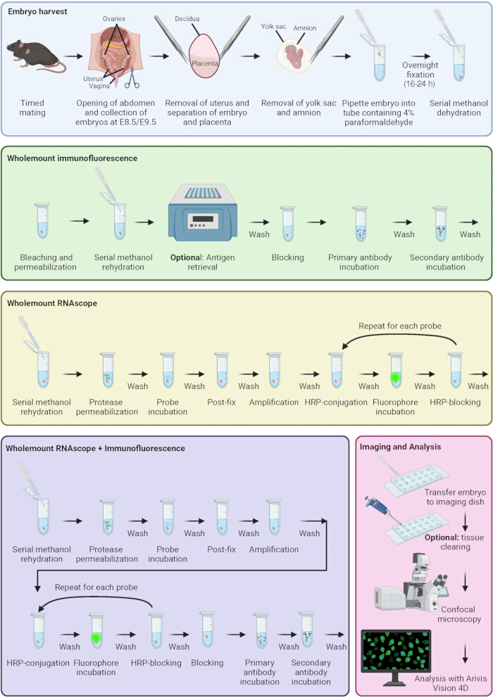
Figure 1: Immunofluorescence and RNAscope staining protocol. Schematic representing key stages of embryo harvest, immunofluorescence, RNAscope, combined immunofluorescence and RNAscope, sample imaging, and analysis. Colored boxes correspond to different protocol stages. Created in BioRender. Sparrow, D. (2026) https://BioRender.com/q6rmax8 Please click here to view a larger version of this figure.

Results

E8.5 embryos were stained by immunofluorescence following this protocol to analyze the number of migrating neural crest cells that were in the G2/M phase of the cell cycle. Samples were stained using antibodies targeting PHH3 to visualize the G2/M phase of the cell cycle and SOX10 to visualize migrating neural crest cells. Embryos were further stained with appropriate secondary antibodies. Nuclei were stained with DAPI. Samples were imaged using the Olympus SpinSR spinning disk confocal microscope with a 10x objective (NA = 0.4). Images were acquired using a Hamamatsu Orca Fusion BT camera and a 50 µm pinhole spinning disk. Images were captured using the tile and stitch function as Z stacks, with a Z-spacing of 1.99 µm. Neural crest cell delamination and subsequent migration by epithelial to mesenchymal transition (EMT) requires pre-migratory neural crest cells to be in the S or G2/M stage of the cell cycle²⁰. Here, we are able to visualize cells in the G2/M phase of the cell cycle, indicated by PHH3 staining (green), within the population of migratory neural crest cells, indicated by SOX10 (magenta) (Figure 2A). The number of migrating neural crest cells in G2/M in control and treatment-exposed embryos can be quantified to determine if our treatment affects the number of migratory neural crest cells in G2/M, and therefore whether our treatment may also perturb neural crest delamination by EMT. Some embryos had a residual yolk sac attached from dissection (Figure 2A’, red arrowhead). The residual yolk sac is sensitive to staining by anti-mouse secondary antibodies, prevalent in this sample, as the anti-PHH3 antibody was raised in a mouse. Thus, the entire yolk sac fluoresces brightly with the fluorophore conjugated to the anti-mouse antibody. In this extreme example, the non-specific staining could affect the quantification of PHH3, and therefore, this sample should be excluded from analysis. Furthermore, the use of anti-mouse antibodies leaves a non-specific ‘streak’ adjacent to the heart tube in E8.5 embryos (Figure 2A’, red arrowhead). This region should be accounted for when quantifying the signal from a primary antibody raised in a mouse.

E9.5 embryos were stained by immunofluorescence using this protocol to examine blood vessel structure and cardiac progenitor cell distribution. Samples were stained using antibodies targeting ISLET1 (ISL1) to visualize the second heart field, SOX10 to visualize migrating neural crest cells, ENDOMUCIN (EMCN) to visualize venous and capillary endothelial cells, and appropriate secondary antibodies. Nuclei were stained with DAPI. Tissue clearing was used to obtain better depth of imaging. Samples were imaged using an Olympus SpinSR spinning disk microscope with a 10x objective (NA = 0.4). At E9.5, we see migration of cardiac neural crest cells, which form part of the aortic arch (SOX10, yellow), and second heart field progenitor cells (ISL1, green), which form parts of the atria, the outflow tract, and the left ventricle²¹ (Figure 2B). Disruption of cardiac progenitor cells is a key driver of congenital heart disease^22,23. Using this method, we are able to visualize cardiac progenitor cell patterning and number. The next stage would be to compare the patterning of cardiac progenitor cells between control and treatment groups to determine if our intervention perturbs migration or leads to loss of key cell types.

To determine the relationship between neural crest cell stage and Wnt signaling, E8.5 embryos were stained by RNAscope using this protocol to examine neural crest cells in different stages of migration and differentiation, and a Wnt signaling marker. Probes indicating the neural plate border, from where neural crest cells emerge (Msx1), migratory neural crest cells (Sox10), and neural crest cell differentiation (Dlx2) were used and compared to a probe indicating Wnt signaling (Sp5). TSA-vivid 520, 570, and 650, and Opal 780 fluorophores were used to visualize probes. Samples were imaged using an Evident FV4000 microscope with a 10x objective (NA=0.4), 144 µm pinhole, and a pixel size of 621 nm. Images were captured using the tile and stitch function as Z stacks, with a Z-spacing of 4.32 µm. The neural plate border (Msx1, green) and migratory neural crest cells (Sox10, magenta) occupy distinct regions in the head, with some overlap as cells begin to migrate from the neural tube (Figure 3A). Some regions of migrating neural crest cells are co-localized with Dlx2 (cyan), suggesting some cells are progressing towards craniofacial differentiation (Figure 3A). Wnt signaling (Sp5, yellow) occupies regions of the neural plate border, which is pertinent as modulation of Wnt signaling is required for neural crest cell delamination and differentiation^24,25, but also a distinct region adjacent to the migratory neural crest cells (Figure 3A).

Further staining aimed to look at the relationship between neural crest cell migration and Wnt signaling at E9.5 by staining for markers of neural crest state and Wnt signaling. Probes indicating the neural plate border (Msx1) and migratory neural crest cells (Sox10) were used and compared to a probe indicating Wnt signaling (Sp5). TSA-vivid 520, 570, and 650 fluorophores were used to visualize probes. Samples were imaged using an Olympus SpinSR spinning disk microscope with a 10x objective (NA = 0.4). Here we can see the neural plate border (Msx1, green), distinct from migrating neural crest cells (Sox10 magenta) (Figure 3B). Wnt signaling (Sp5, yellow) can be seen strongly in the dorsal region of the embryo, where trunk neural crest cells are delaminating, as well as in distinct regions in the head, around the 1^st and 2^nd branchial arch, below the outflow tract, and within the otic vesicle (Figure 3B). Comparing the spatial patterning of neural crest cells and Wnt signaling between control and treatment groups using this method would allow us to determine whether our intervention perturbs neural crest cell delamination and migration, and whether any perturbation is due to alterations in Wnt signaling.

To determine the cell cycle state of cells in the neural plate border, we used this protocol to combine immunofluorescence and RNAscope staining. An RNAscope probe indicating the neural plate border (Msx1) was used. Samples were stained using antibodies targeting PHH3 and PCNA to visualize the G2/M and S-phases of the cell cycle, respectively. Embryos were further stained with appropriate secondary antibodies. Nuclei were stained with DAPI. Samples were imaged using the Olympus SpinSR spinning disk microscope with a 10x objective (NA = 0.4) (Figure 4A,B), or an Evident FV4000 confocal microscope with a 10x objective (NA = 0.4), 127 µm pinhole, and a pixel size of 311 nm. (Figure 4B’). Here we can see cells in both G2/M (PHH3, yellow) and S-phase (PCNA, magenta) overlapping with the neural plate border (Figure 4A). Using this method, we can quantify the proportion of cells within the neural plate border in each stage of the cell cycle and determine if these proportions are altered by our treatment groups. Notable in this embryo are holes that result from dissection damage to the embryo by excessive manipulation of the embryo using fine forceps. This highlights the need for care in dissection to prevent damage, particularly at E8.5 when the embryos are particularly fragile.

Combining RNAscope and immunofluorescence can lead to dimmer staining of the RNAscope probe than performing RNAscope alone. When combined with a primary antibody that is very brightly fluorescing with a nearby fluorophore (e.g., Fluorescein and Cy3), this can lead to bleed-through of signal from the brighter to the dimmer channel (Figure 4B). The way to prevent this is to use a more dilute concentration of the very bright antibody, selecting fluorophores that are more spectrally distinct, or to change imaging parameters in samples. Spinning disk microscopes are very fast at imaging embryos, but as they utilize band-pass emission filters with fixed emission windows, there is no way of narrowing detection windows dynamically to match specific fluorophores. Using a point-scanning microscope, e.g., Evident FV4000, the detection window can be narrowed by the operator with nanometer precision, so bleed-through can be reduced when fluorophores are used that have a slight overlap in emission spectra (Figure 4B’).

To determine which proportions of cells were in different stages of the cell cycle in E8.5 embryos, we used this protocol to analyze the proportion of nuclei and intensity of signal in both the S-phase and G2/M phase of the cell cycle. Samples were stained using antibodies targeting PHH3 and PCNA to visualize the G2/M and S-phases of the cell cycle, respectively. Embryos were further stained with appropriate secondary antibodies. Nuclei were stained with DAPI. Samples were imaged using the Olympus SpinSR spinning disk microscope with a 10x objective (NA = 0.4). Zeiss Arivis Pro was used to identify all nuclei, nuclei positive for PHH3, nuclei positive for PCNA, and double-positive nuclei (Figure 5A). Using this method, we were able to compare the proportions of cells in G2/M (PHH3⁺) and S (PCNA⁺) phases of the cell cycle (Figure 5B), and the intensity of PHH3 or PCNA staining in each individual nucleus (Figure 5C). We can see that there was a slightly higher proportion of PCNA⁺ nuclei in the heart region compared to the head and whole embryo (Figure 5B). Furthermore, the head had a higher proportion of PHH3⁺ and double-stained nuclei compared to the heart and the whole embryo (Figure 5B). There were no overt differences in intensity of PHH3 or PCNA between regions (Figure 5C). These data are derived from a single representative embryo (n = 1) and are presented to demonstrate the analysis workflow; no inferential statistical analysis was performed. Together, this method allows us to determine patterns of cell cycle propagation at a stage of development crucial for cardiac and craniofacial development. This method will allow us to determine if our treatment affects cell cycle propagation in different regions of the embryo.

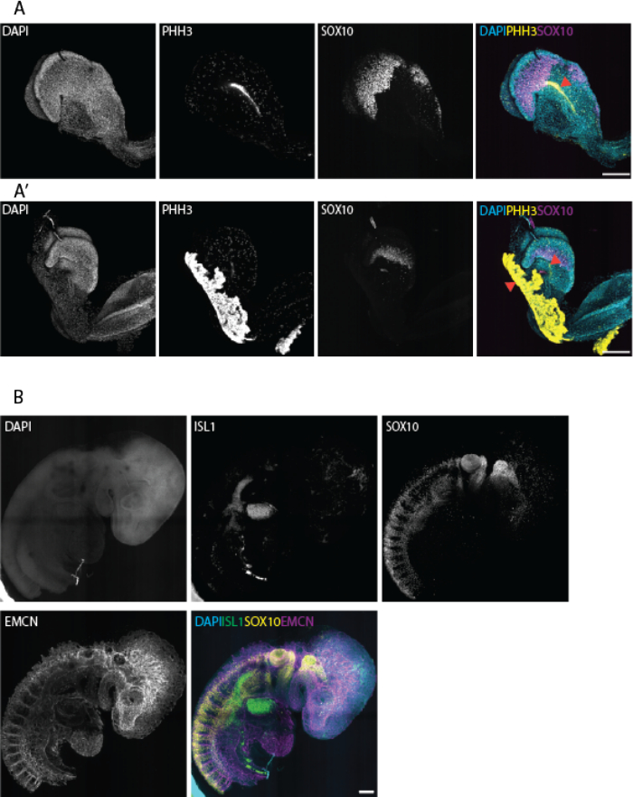
Figure 2: Immunofluorescence staining of proteins in E8.5 and E9.5 embryos. (A, A’) E8.5 mouse embryos were stained by immunofluorescence for PHH3 to visualize cells in the G2/M-phase of cell cycle, SOX10 to visualize migrating neural crest cells, and DAPI to visualize nuclei. N = 11 embryos from 1 experiment. (B) E9.5 embryos were stained for ISL1 to visualize second heart field progenitors, SOX10 to visualize migrating neural crest cells, EMCN to visualize capillary and venous blood vessels, and DAPI (to visualize nuclei. Red arrowheads indicate non-specific staining of the yolk sac, and non-specific staining within the embryo from anti-mouse secondary antibodies (n = 15 embryos from 1 experiment). Scale bar = 200 µm. DAPI: 4′,6-diamidino-2-phenylindole; PHH3: Phosphohistone H3; EMCN: Endomucin. Please click here to view a larger version of this figure.

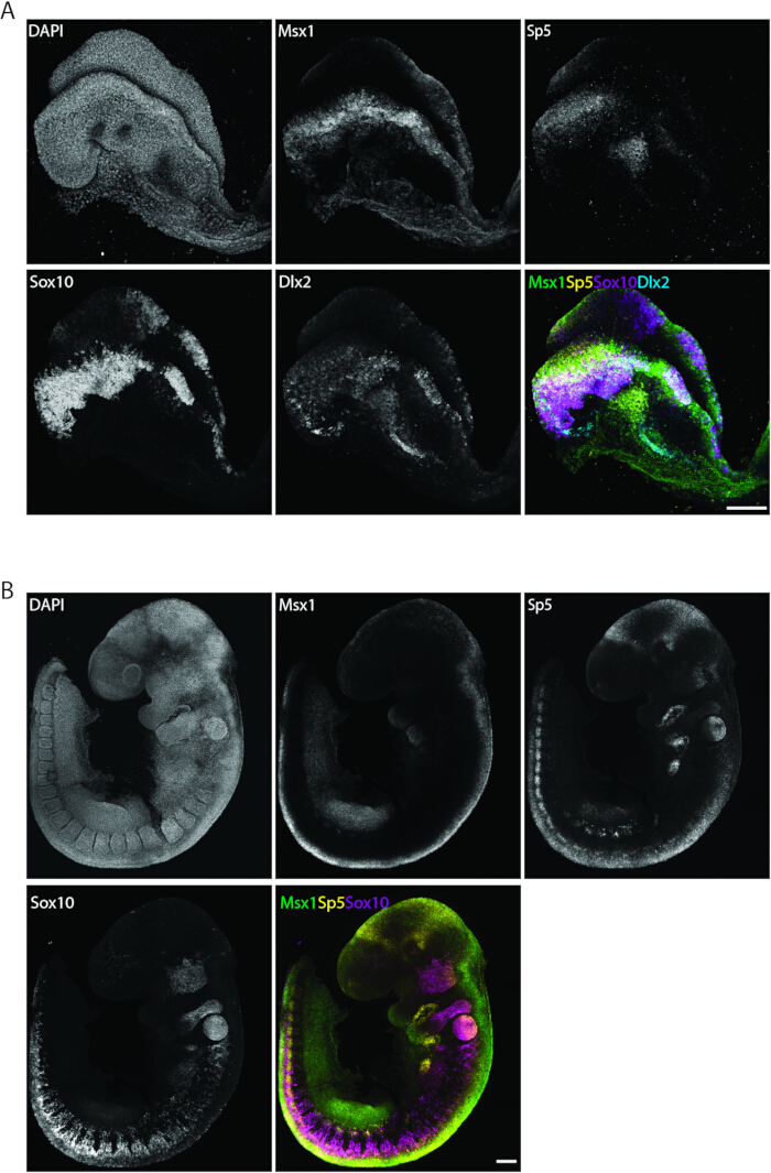
Figure 3: Staining transcripts in E8.5 and E9.5 embryos by RNAscope. (A) E8.5 embryos were stained by RNAscope for probes targeting Msx1 to visualize the neural plate border, Sox10 to visualize migrating neural crest, Dlx2 to visualize differentiating neural crest, and Sp5 for Wnt signaling. n = 13 embryos from 1 experiment. (B) E9.5 embryos were stained by RNAscope for probes targeting Msx1 to visualize the neural plate border, Sox10 to visualize migrating neural crest, and Sp5 to visualize Wnt signaling. n = 4 embryos from 1 experiment. Scale bar = 200 µm. Please click here to view a larger version of this figure.

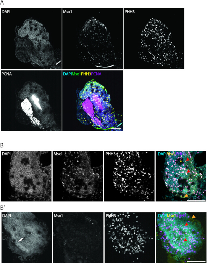
Figure 4: Combined immunofluorescence staining and RNAscope in E8.5 embryos. (A, B, B’) E8.5 embryos were stained by RNAscope for probes targeting Msx1 to visualize the neural plate border and by immunofluorescence for PCNA to visualize cells in S-phase and PHH3 antibodies to visualize cells in G2/M phase of the cell cycle. Orange arrowheads indicate specific Msx1 staining, red arrowheads indicate bleed-through fluorescence, (B), or specific PHH3 staining without bleedthrough into the Msx1 channel (B'). N = 2 embryos from 1 experiment. Scale bar = 200 µm. Please click here to view a larger version of this figure.

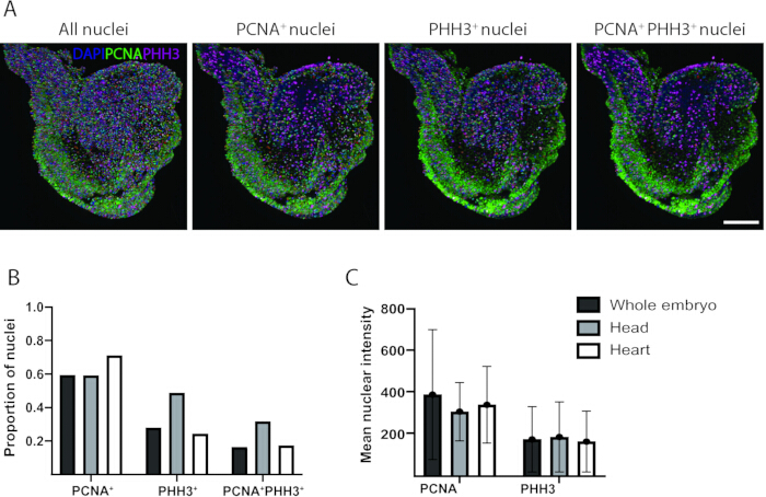
Figure 5: Analysis of cell cycle stage in E8.5 embryos using Arivis Pro. (A) E8.5 mouse embryos were stained by immunofluorescence for PCNA to visualize cells in S-phase of the cell cycle (green), PHH3 to visualize cells in G2/M phase of the cell cycle (magenta), and DAPI to visualize nuclei (blue). Detected 3D objects (multicolored spheres) were overlaid and visualized using the 4D viewer in Zeiss Arivis Pro. (B) The graph demonstrates the proportion of PCNA⁺, PHH3⁺, and double-positive nuclei in the whole body, head, and heart of a single embryo. (C) The graph demonstrates the mean intensity of PCNA and PHH3 staining per nucleus in the whole body, head, and heart of a single embryo. Circles represent the mean; error bars represent the standard deviation of all nuclei within a single sample. Graphs were made using GraphPad Prism. Scale bar = 200 µm. Quantitative analysis was performed on n = 1 embryo. No inferential statistics were performed. Error bars indicate standard deviation between individual nuclei. 3D: Three-dimensional; DAPI: 4′,6-diamidino-2-phenylindole. Please click here to view a larger version of this figure.

Discussion

Here, we describe an optimized method of analyzing gene and protein expression spatially within whole-mount E8.5 and E9.5 embryos. These methods have improved spatial resolution and multiplexing ability compared to traditional methods of RNA in situ hybridization and immunofluorescence of sections. This protocol builds upon existing recent protocols to examine developmental pathways in mouse embryos. One recent protocol used RNAscope and immunofluorescence staining to look at Wnt signaling in embryos, but stained sections rather than whole-mount embryos²⁶. Another recent study performed whole-mount RNAscope and immunofluorescence staining on E8.5–E10.5 whole-mount mouse embryos²⁷, but the authors did not combine the two staining techniques, nor was a fourth RNAscope channel stained for using C4 probes and Opal 780 fluorophores. Combined immunofluorescence and RNAscope has previously been described in whole-mount E3.5 embryos, where RNAscope is performed after completing the immunofluorescence protocol²⁸. Whilst we have not tried this exact protocol in later embryos, we achieved poor antibody staining when sandwiching RNAscope staining between the primary and secondary antibody incubations of our immunofluorescence protocol in E8.5 embryos. This is likely due to the need to use a protease incubation when performing RNAscope on larger embryos, which was not required in the study using E3.5 mouse embryos. Protease incubation could affect the integrity of bound antibodies, thus swapping the order of RNAscope and immunofluorescence is unlikely to work in this system. A further recent study in myofibers combined the two protocols by performing RNAscope prior to immunofluorescence staining²⁹. Similarly to this protocol, that study performed RNAscope before immunofluorescence; however, the method was not validated their protocol in whole-mount mouse embryos, nor had they performed RNAscope incorporating an additional RNAscope channel by staining with C4 probes and an Opal 780 fluorophore.

The ability to stain whole-mount embryos using multiplexing has wide-reaching applications for developmental biology to be able to map key transcripts and proteins, labeling progenitor cell types or developmental signaling pathways in embryos at different stages. We have been able to use these techniques to map cardiac progenitor cell distribution (Figure 2B), neural crest cells at different stages of migration and differentiation (Figure 3), Wnt signaling (Figure 3), and cell cycle stage (Figure 2, Figure 4, Figure 5). By modifying the probes and antibodies used, it is possible to use these techniques to examine any cell types or signaling molecules of interest as long as they exist in the embryos at this stage. Although we have focused on E8.5 and E9.5 in this protocol, it is possible that younger or older embryos can also be stained by modification of tissue permeabilization, incubation times, and tissue clearing.

However, this enhanced ability to multiplex protein and transcript expression in whole-mount embryos has led to further challenges. Firstly, performing analysis on whole-mount samples is time-consuming compared to immunofluorescence and RNAscope on sections, which can typically be performed over 1–2 days rather than multiple days. Furthermore, the use of whole-mount samples requires careful consideration of microscopy parameters to ensure adequate sample depth and resolution. A microscope is needed that can image through as much as 700 µm thick tissue, and tissue clearing needs to be used in larger embryos, otherwise structures deep in the sample may be missed. In addition, due to the thickness of the samples, imaging with a widefield microscope would lead to a large amount of light from outside of the focal plane being imaged; a confocal microscope is preferred due to its ability to remove signals from outside the focal plane, thus it can image through the sample whilst excluding any out-of-plane signal. Additionally, a spinning disk confocal microscope often allows quicker image acquisition times, but compromises on fine control of fluorescence detection compared to a point-scanning confocal microscope. The size of the embryos can also be challenging, as many microscopes do not have a field of view large enough to image the embryo without tile-scanning. This can lead to stitching artifacts within the image (e.g., Figure 2B). Multiplexing samples might also lead to bleed-through between channels (e.g., Figure 4B), which can be mitigated by selecting a point-scanning confocal microscope where detection windows can be narrowed, where fluorophores have slight overlaps in emission spectra. The use of the Opal 780 fluorophore is useful to multiplex even more targets in a single sample; a microscope that has the ability to image near-infrared is needed to detect this system. This ability is not available on the majority of light microscopes.

Mounting the samples for imaging also requires careful consideration. By allowing the samples to free float, such as when imaging in a multi-well chamber slide, the samples are not always at exactly the same angle for imaging. This can lead to differences in intensity of staining depending on which parts of the embryo are closest to the camera/detector, and can lead to challenges when performing downstream intensity analysis. A further issue with using multi-well chamber slides is that the edge of the well might be within the field being imaged, which can lead to artifacts in the image. Pinning the embryo down, such as in a cavity slide, can help to maintain orientation, but can make it easy to damage and/or compress the embryo, making volume analysis of structures challenging.

Several considerations need to be made when following this protocol. For immunofluorescence, care needs to be taken during antigen retrieval not to dissociate the embryo, especially when analyzing younger embryos. To avoid this, it may be possible to use other antigen retrieval methods, such as using an alternative buffer like Tris/EDTA or using a proteolytic retrieval method. Smaller or larger embryos might benefit from optimization of antibody incubation times. Careful consideration of primary antibodies is needed, as several antibodies are raised in mice, but the use of anti-mouse antibodies can bind residual yolk sac and fluoresce brightly. This can be seen using anti-mouse secondaries bound to AlexaFluor 488 (Figure 2) and AlexaFluor 647 (Figure 4). Other fluorophores have not been tested in our lab, but these may have differing intensities of fluorescence, requiring further optimization. This effect is not seen in channels where anti-rabbit (Figure 2, Figure 4, Figure 5) or anti-rat antibodies (Figure 2B) have been used; therefore, the use of primary antibodies raised in other species is recommended where possible.

For RNAscope, it is critically important to optimize the protease incubation steps, as too little time can lead to insufficient penetration of probes, and too long can lead to complete dissociation of the sample. When optimizing protease incubation times, we recommend modifying the duration by a single minute at a time. It is best practice to also use appropriate controls to determine whether or not a probe or antibody has worked. A negative control would be an embryo of equivalent stage and stained together that has had no probe/no primary antibody, or use of an IgG isotype control or a negative control probe for immunofluorescence or RNAscope, respectively, to determine that observed staining is real. Positive controls of an equivalent-sized tissue known to express the gene or transcript of interest can also be useful to determine whether staining has been successful.

Overall, this protocol is a robust, optimized method for visualizing protein and transcript expression in whole-mount mouse embryos at E8.5 and E9.5, with great potential for investigating cellular and molecular mechanisms in normal embryonic development and disease.

Materials

List of materials used in this article

Name	Company	Catalog Number	Comments
Plasticware/glassware
3ml Pasteur pipettes Low-density Polyethylene (LDPE) graduated	Wheaton	711116
Eppendorf Safe-lock tubes 1.5ml microtube	Eppendorf	0030 120.086
Ibidi µ-slide 18-well	Ibidi	81817	#1.5H glass coverslip, untreated
Menzel X1000 Coverslip 22x50 mm #1.5 (0.16-0.19mm)	Thermo Scientific	17284904
Microscope slides with cavities	Marienfeld Superior	1320000
Safe seal microtube 2ml	Sarstedt	72.695.500	2ml 'Eppendorf' tube, round bottomed
Solutions/buffers
1x Antibody diluent/block	Akoya Biosciences	ARD1001EA
Ambion™ RnaseZap™ Rnase Decontamination Solution	Ambion	9780.9782
Citrate unmasking buffer	Vector labs	H-3300	Labelled as Antigen unmasking solution, citric acid based
Dimethyl sulfoxide (DMSO)	Merck (Sigma-Aldrich)	D8418
Hanks' Balanced Salt Solution 10x	Merck (Sigma-Aldrich)	H4641
Hydrogen peroxide solution	Merck (Sigma-Aldrich)	H1009	30% (w/w) in H2O
Methanol	Merck (Sigma-Aldrich)	32213-2.5L-M
Normal donkey serum	Abcam	Ab7475	100% stock concentration, 10% final concentration
Paraformaldehyde (PFA) powder	Merck (Sigma-Aldrich)	158127-500g	Dilute to 4% in water. Prepare in fume hood. Stir on heated block and add a small amount of NaOH to facilitate dissolving. pH 7.2-7.6
Phospho buffered saline (PBS)	Merck (Sigma-Aldrich)	P4417	1 tablet per 200ml distilled water
RNAscope 4-Plex Ancillary Kit for Multiplex Fluorescent Reagent Kit v2	ACD (Bio-Techne)	323120	Contains HRP-C4 and HRP blocker
RNAscope™ Multiplex Fluorescent Detection Kit v2	ACD (Bio-Techne)	323110	Contains Protease Plus, Protease III, Protease IV, hydrogen peroxide, TSA buffer, Amp1/2/3, Hrp-C1/2/3, HRP-blocker and DAPI
Saline-Sodium-Citrate (SSC) buffer 20X solution	Fisher Bioreagents	BP-1325-1	Dilute to 0.2x in distilled water
Tissue-Clearing Reagent Cubic-R+(M) [for animals]	Tokyo Chemical Industry	T3741
Triton™ X 100	Merck (Sigma-Aldrich)	X100
Tween® 20	Merck (Sigma-Aldrich)	P7949
Ultrapure™ 0.5M EDTA, pH8	Invitrogen	15575020
Primary antibodies
Endomucin antibody (V.7C7)	Santa Cruz	SC-65495	Use 1:50 dilution.
Islet 1 and Islet 2 antibody	Developmental Studies Hybridioma Bank	34.4DS-5	Dilute 50% in glycerol. Use 1:50 dilution.
PCNA (PC10) Mouse Monoclonal antibody	Cell Signaling Technology	2586S	Use 1:500 dilution
P-histone H3 (Ser10) (6G3) Mouse Monoclonal antibody	Cell Signaling Technology	9706S	Use 1:500 dilution
P-histone H3 (Ser10) (D7N8E) XP® Rabbit Monoclonal antibody	Cell Signaling Technology	53348S	Use 1:500 dilution
Sox10 (E6B6I) XP® Rabbit Monoclonal Antibody	Cell Signaling Technology	69661S	Use 1:500 dilution
Secondary antibodies/nuclear stains
AlexaFluor® 488-conjugated Affinipure® Donkey anti-mouse IgG (H+L)	Jackson Immunoresearch	715-545-151	Use 1:500 dilution
AlexaFluor® 647-conjugated Affinipure®  Donkey anti-rat IgG (H+L)	Jackson Immunoresearch	712-605-153	Use 1:500 dilution
AlexaFluor® 647-conjugated Affinipure® F(ab')2 Fragment Donkey anti-mouse IgG (H+L)	Jackson Immunoresearch	715-606-150	Use 1:500 dilution
Cy™3 Affinipure® Donkey anti-Rabbit IgG (H+L)	Jackson Immunoresearch	711-165-152	Use 1:500 dilution
DAPI	Merck (Sigma-Aldrich)	D9542	Used at 1 µg/ml
RNAscope probes
RNAscope® Probe - Mm Sp5-C4	ACD (Bio-Techne)	405681-C4	C4 probe
RNAscope® Probe - Mm-Dlx2-C3	ACD (Bio-Techne)	555951-C3	C3 probe
RNAscope® Probe - Mm-Msx1	ACD (Bio-Techne)	421841	C1 probe
RNAscope® Probe - Mm-Sox10-C2	ACD (Bio-Techne)	435931-C2	C2 probe
RNAscope flurophores
Opal 780 Reagent Pack	Akoya Biosciences	FP1501001KT	Contains Opal 780 reagent, Opal TSA-DIG, DMSO
TSA-vivid™ fluorophore 520	ACD (Bio-Techne)	323271	now ClariTSA™ fluorophore 520
TSA-vivid™ fluorophore 570	ACD (Bio-Techne)	323272	now ClariTSA™ fluorophore 570
TSA-vivid™ fluorophore 650	ACD (Bio-Techne)	323273	now ClariTSA™ fluorophore 650
Equipment/software
Fluoview FV4000 laser scanning  microscope	Evident	fv4000	Excitation lasers: 405/488/561/640/730 nm. Detected wavelength (Fig. 3): 430-470, 500-540, 570-620, 650-710, 750-850 nm. Detected wavelength (Fig. 4) 430-470, 500-531, 570-620 nm.
Graphpad Prism 10	Graphpad		v10.6.1
Heating block	Grant	QBT1
Hybrigene hybridisation oven	Techne (Bibby Scientific)	FHB4DD
Ixplore IX83 SpinSR Super-Resolution Microscope System	Olympus	ixplore-ix83-spinsr	Excitation lasers: 405/488/561/640 nm. Emission filters: 447/60, 525/50, 617/73, 685/40.
Zeiss Arivis Pro	Carl Zeiss Microscopy GmbH		v. 4.5 (previously Arivis Vision 4D)
Zeiss Arivis SIS converter	Carl Zeiss Microscopy GmbH		v. 4.3.0

References

- Bruter AV, Varlamova EA, Okulova YD, Tatarskiy VV, Silaeva YY, Filatov MA. Genetically modified mice as a tool for the study of human diseases. Mol Biol Rep. 2024;51(1):135.
- Rashbrook VS, Brash JT, Ruhrberg C. Cre toxicity in mouse models of cardiovascular physiology and disease. Nat Cardiovasc Res. 2022;1:806–16.
- Breschi A, Gingeras TR, Guigo R. Comparative transcriptomics in human and mouse. Nat Rev Genet. 2017;18(7):425–40.
- Mole MA, Weberling A, Zernicka-Goetz M. Comparative analysis of human and mouse development: From zygote to pre-gastrulation. Curr Top Dev Biol. 2020;136:113–38.
- Krishnan A, Samtani R, Dhanantwari P, Lee E, Yamada S, Shiota K, et al. A detailed comparison of mouse and human cardiac development. Pediatr Res. 2014;76(6):500–7.
- Anderson RH, Bamforth SD. Morphogenesis of the Mammalian Aortic Arch Arteries. Front Cell Dev Biol. 2022;10:892900.
- Wessels A, Sedmera D. Developmental anatomy of the heart: a tale of mice and man. Physiol Genomics. 2003;15(3):165–76.
- Gall JG, Pardue ML. Formation and detection of RNA-DNA hybrid molecules in cytological preparations. Proc Natl Acad Sci U S A. 1969;63(2):378–83.
- John HA, Birnstiel ML, Jones KW. RNA-DNA hybrids at the cytological level. Nature. 1969;223(5206):582–7.
- Buongiorno-Nardelli M, Amaldi F. Autoradiographic detection of molecular hybrids between RNA and DNA in tissue sections. Nature. 1970;225(5236):946–8.
- Dakou E, Vanbekbergen N, Corradi S, Kemp CR, Willems E, Leyns L. Whole-mount in situ hybridization (WISH) optimized for gene expression analysis in mouse embryos and embryoid bodies. Methods Mol Biol. 2014;1211:27–40.
- Anderson R. Multiplex fluorescence in situ hybridization (M-FISH). Methods Mol Biol. 2010;659:83–97.
- Kearney L. Multiplex-FISH (M-FISH): technique, developments and applications. Cytogenet Genome Res. 2006;114(3-4):189–98.
- Burnett R, Guichard Y, Barale E. Immunohistochemistry for light microscopy in safety evaluation of therapeutic agents: an overview. Toxicology. 1997;119(1):83–93.
- Coons AH, Creech HJ, Jones RN. Immunological properties of an antibody containing a fluorescent group. P Soc Exp Biol Med. 1941;47(2):200–2.
- Bardot E, Tzavaras N, Benson DL, Dubois NC. Quantitative Whole-mount Immunofluorescence Analysis of Cardiac Progenitor Populations in Mouse Embryos. J Vis Exp. 2017(128).
- Wang F, Flanagan J, Su N, Wang LC, Bui S, Nielson A, et al. RNAscope: a novel in situ RNA analysis platform for formalin-fixed, paraffin-embedded tissues. J Mol Diagn. 2012;14(1):22–9.
- Erben L, Buonanno A. Detection and Quantification of Multiple RNA Sequences Using Emerging Ultrasensitive Fluorescent In Situ Hybridization Techniques. Curr Protoc Neurosci. 2019;87(1):e63.
- De Bono C, Lescroart F, Zaffran S. How to Study Gene Expression and Gain of Function of Hoxb1 in Mouse Heart Development. Methods Mol Biol. 2025;2889:121–37.
- Zhao R, Moore EL, Gogol MM, Unruh JR, Yu Z, Scott AR, et al. Identification and characterization of intermediate states in mammalian neural crest cell epithelial to mesenchymal transition and delamination. Elife. 2024;13.
- Guijarro C, Kelly RG. On the involvement of the second heart field in congenital heart defects. C R Biol. 2024;347:9–18.
- Bradshaw L, Chaudhry B, Hildreth V, Webb S, Henderson DJ. Dual role for neural crest cells during outflow tract septation in the neural crest-deficient mutant Splotch(2H). J Anat. 2009;214(2):245–57.
- Zawada D, Kornherr J, Meier AB, Santamaria G, Dorn T, Nowak-Imialek M, et al. Retinoic acid signaling modulation guides in vitro specification of human heart field-specific progenitor pools. Nat Commun. 2023;14(1):1722.
- Rabadan MA, Herrera A, Fanlo L, Usieto S, Carmona-Fontaine C, Barriga EH, et al. Delamination of neural crest cells requires transient and reversible Wnt inhibition mediated by Dact1/2. Development. 2016;143(12):2194–205.
- Bhattacharya D, Rothstein M, Azambuja AP, Simoes-Costa M. Control of neural crest multipotency by Wnt signaling and the Lin28/let-7 axis. Elife. 2018;7.
- Kishimoto K, Furukawa KT, Luz-Madrigal A, Yamaoka A, Matsuoka C, Habu M, et al. Bidirectional Wnt signaling between endoderm and mesoderm confers tracheal identity in mouse and human cells. Nat Commun. 2020;11(1):4159.
- De Bono C, Liu Y, Ferrena A, Valentine A, Zheng D, Morrow BE. Single-cell transcriptomics uncovers a non-autonomous Tbx1-dependent genetic program controlling cardiac neural crest cell development. Nat Commun. 2023;14(1):1551.
- Hazra R, Spector DL. Simultaneous visualization of RNA transcripts and proteins in whole-mount mouse preimplantation embryos using single-molecule fluorescence in situ hybridization and immunofluorescence microscopy. Front Cell Dev Biol. 2022;10:986261.
- Kann AP, Krauss RS. Multiplexed RNAscope and immunofluorescence on whole-mount skeletal myofibers and their associated stem cells. Development. 2019;146(20).
Reprints and Permissions
This article has been published
Video Coming Soon