Machine Learning Outperforms Deep Learning for Atmospheric Attenuation Prediction in Free-Space Optical Communications under Iraqi Weather Conditions

Summary

This protocol describes the generation of a weather-based dataset and the systematic evaluation of machine learning, deep learning, and hybrid models for predicting atmospheric attenuation in free-space optical communications under diverse Iraqi environmental conditions, including dust storms, fog, rain, and snow.

Abstract

Free-space optical communications systems offer high bandwidth, increased security and license-free operation but are highly affected by the performance degradation due to the atmospheric attenuation caused by scattering and absorption. The prediction of attenuation accuracy is even more important in Iraq where the environment is hot, dusty, foggy and rainy in a random fashion. The aim of this study is to assess the performance of machine learning, deep learning and hybrid modeling techniques for the prediction of free-space optical communication systems atmospheric attenuation in different Iraqi weather conditions. A synthetic dataset of 1500 samples was created using well established physical propagation models for five weather regimes: clear sky, fog, rain, dust storms and snow. Fifteen predictive models were systematically evaluated, consisting of six machine learning techniques (Random Forest [RF], Extreme Gradient Boosting, Light Gradient Boosting Machine, Support Vector Regression, Linear Regression, and K-Nearest Neighbors), six deep learning architectures (Multilayer Perceptron, Deep Neural Network, Long Short-Term Memory [LSTM], One-Dimensional Convolutional Neural Network [CNN], CNN–LSTM, and Attention-based Network) and three hybrid approaches. The results showed that RF performed the best (R² = 0.9654, root mean square error = 1.324 dB/km) compared to deep learning approaches (best R² = 0.7766) and hybrid methods (best R² = 0.9571). The feature importance was analyzed by Shapley Additive exPlanations and dust concentration (67.3%) and visibility (21.2%) were found to be the most influential factors. While RF resulted in substantially faster training and inference , statistical testing revealed no significant difference between RF and the best performing hybrid approach (p = 0.083). The performance of the conventional machine learning techniques is proved to be highly efficient for the estimation of atmospheric attenuation in FSO communication systems in adverse environmental conditions in agreement with well known physical propagation theories. However, we stress that these conclusions are based on synthetic data, and must be validated by real atmospheric measurements before they can be used in operational FSO systems.

Introduction

Free-space optical (FSO) communication networks generally offer higher capacity and better security, but atmospheric attenuation due to scattering and absorption is a major limiting factor for the communication distance¹. In this work we provide a detailed analysis of machine-learning, deep-learning and hybrid approaches² to assess FSO signal attenuation in the challenging environment of Iraq, with high temperatures, dust storms and irregular rainfall.

The FSO communication systems have emerged as one of the promising solutions for high-bandwidth wireless connectivity³ with data rates exceeding 100 Gbps over distances from hundreds of meters to few kilometers⁴. FSO links operate in the visible and infrared spectrum, unlike conventional radio-frequency systems, offering benefits such as license-free operation, immunity to electromagnetic interference, improved security through narrow beam divergence and large bandwidth capacity⁵. These features make FSO an attractive technology for backhaul applications, interbuilding links, disaster recovery networks, and last mile connectivity where fiber deployment is prohibitively expensive⁶. But communication via scattering, beam deflection and absorption^7,8 is heavily dependent on environmental conditions in terms of availability and performance. This challenge is one of the major constraints of free-space optical communication systems. Weather conditions cause wide variations in attenuation levels (dB/km). Under clear-sky conditions, attenuation can be less than 0.5 dB/km, while severe fog may cause attenuation to reach ≥50 dB/km at 1550 nm (using the Kim fog model, which predicts attenuation values up to 50 dB/km for visibility below 50 m at 1550 nm)^9,10 and heavy rain can cause attenuation to reach up to 20–30 dB/km depending on the rainfall rate (Carbonneau model prediction)¹¹. Thus accurate prediction of the attenuation is needed for reliable link design, network planning and adaptive transmission strategies. The conventional methods are based on physical propagation models, such as the Kim model for fog¹², the Carbonneau model for rain¹³, and Mie scattering theory for aerosol particles¹⁴. However, while these models provide a good theoretical foundation, they often rely on accurate atmospheric parameters that are not always available in practice, and frequently do not consider the complex interactions between concurrent multiple meteorological phenomena¹⁵.

The extreme environmental variability in Iraq presents significant challenges to the deployment of free-space optical communication systems. Transmission circumstances are further complicated by minimal rainfall and isolated fog episodes, while winter temperatures can drop below freezing and summer temperatures can rise beyond 50 °C¹⁶. At regularly utilized spectrum like 1550 nm in normal wavelengths, dust storms, referred to locally as "al-haboob," can restrict sight to less than 100 meters, leading in attenuation values exceeding 20dB/km¹⁷. For FSO systems to be successfully deployed in Iraq and other Middle Eastern nations, it is necessary to create trustworthy prediction models that can precisely estimate the system's performance under these different environmental conditions¹⁸.

New developments in machine learning present viable substitutes for conventional physics-based modeling techniques. The ability of machine learning techniques to directly learn intricate nonlinear correlations between attenuation and atmospheric factors enables the detection of minute interactions that traditional analytical models could overlook¹⁹. In a variety of climatological prediction tasks, Random Forest (RF) and gradient-boosting strategies have demonstrated strong performance²⁰. Similarly, deep learning techniques have seen remarkable success in natural language processing, computer vision and time-series forecasting²¹. However, these approaches are under-explored for FSO attenuation prediction, in particular with limited datasets and highly variable weather conditions²². To fill this gap, this work presents a thorough investigation of Machine learning, Deep learning and hybrid approaches for predicting FSO signal attenuation in the Iraqi atmospheric conditions. This is achieved by constructing a well-designed synthetic dataset based on well-known physical propagation models²³. We hypothesize that for moderate sized tabular environmental datasets with few dominant predictive variables, the predictive performance of tree-based ensemble methods will outperform complex deep learning architectures. The primary aims are to (1) establish a baseline methodology for the comparison of forecasting methods in a controlled simulation environment, (2) identify the best algorithmic strategies for predicting atmospheric attenuation, and (3) assess feature importance and model interpretability to gain insight into the environmental factors most affecting attenuation. In this work synthetic data are used, but the foundation is laid for later validation with real-world experimental measurements, which is foreseen for future work. Furthermore, feature importance and interpretability analyzes are incorporated to determine the most important environmental factors that influence attenuation.

Protocol

This study did not involve human participants or vertebrate animals, or sampling of tissue. All data used for this research were synthetically generated using physical propagation models and publicly available meteorological parameters. Hence, no ethics approval from an Institutional Review Board (IRB) or Institutional Animal Care and Use Committee (IACUC) was needed.
Dataset Generation Based on the Physical Propagation Theory. The dataset was built to mimic hourly atmospheric conditions for a free-space optical communication system for a whole calendar year (2024) for Iraqi atmospheric conditions. We created a synthetic database with 1,500 samples per hour.

First, weather conditions were randomly assigned based on regional trends: clear sky (54.3%), dust (24.9%), fog (10.5%), rain (7.4%), and snow (2.8%). Secondly, the corresponding physical attenuation model was applied to each sample based on the weather condition, i.e. the Beer-Lambert law for clear sky, the Kim model for fog, the Carbonneau theory for rain and Mie scattering theory for dust storms. Third, the parameters of the FSO system were set as follows: transmission power of 20 dBm, wavelength of 1550 nm, transmission distance of 3 km, transmission aperture of 2.5 cm, and receiving aperture of 20 cm. Fourth, attenuation was computed in dB/km for each sample. Finally, the complete dataset was randomly divided into 1,200 training samples (80%) and 300 testing samples (20%). The simulated conditions include large dust concentrations in association with sandstorms, rainstorms and temperature changes from −4.89°C to 47.99°C. The weather conditions and parameter distributions were selected based on the Iraqi climate records of the period 2020–2024. The five weather regimes (clear sky, fog, rain, dust storms and snow) were chosen because they cover the full spectrum of atmospheric conditions that affect FSO attenuation in Iraq, with dust storms being especially prevalent in the Middle East. The historical data on meteorology gathered throughout Iraqi regions was used to create the probability distribution for each weather condition. The distribution that resulted was as follows: 54.3% of the sky is clear (the predominant state), 24.9% is dust (representing Iraq's sandstorm problem), 10.5% is fog (frequent in northern Iraqi winters), 7.4% is rain (low rainfall amounts typical for Iraq), and 2.8% is snow (sometimes in northern mountainous locations). The relevant meteorological parameters were modeled using probability distributions for each weather condition as follows: temperature was modeled using a normal distribution (mean 28.55±11.18°C) between −4.89°C and 47.99°C based on Iraqi seasonal extremes; humidity was modeled using a uniform distribution (mean 42.01±25.56%) from 0% to 100%; visibility was modeled using a log-normal distribution between 0.05 km and 29.99 km (mean 13.10±10.91 km) to account for the frequent low-visibility events during dust storms; dust concentration was modeled using an exponential distribution between 0 and 4.96 mg/m³ (mean 0.74±1.30 mg/m³) with higher probabilities for low concentrations and long tails for extreme dust events.

The communication system was designed with a transmission power of 20 dBm, a wavelength of 1550 nm, a transmission distance up to 3 km, a transmission aperture of 2.5 cm, and a receiving aperture of 20 cm to compensate for the divergence loss . The parameters of the FSO system were divided into two groups: fixed parameters that did not change for all the samples, and variable parameters that were changed during the generation of the dataset. For all 1,500 samples the following parameters were fixed: transmission power (20 dBm), operating wavelength (1550 nm), transmission aperture (diameter 2.5 cm, efficiency 0.7) and receiving aperture (diameter 20 cm, efficiency 0.7). These parameters were fixed because they are the physical specifications of the FSO system hardware and they do not change with weather conditions. The data set was created with 1500 samples with the following parameters varied: temperature (−4.89°C to 47.99°C), humidity (0% to 100%), visibility (0.05 km to 29.99 km), dust concentration (0 to 4.96 mg/m³) and weather condition (clear sky, fog, rain, dust, snow). These parameters were modified according to probability distributions derived from Iraqi climate records for the years 2020–2024. For each sample the attenuation value (dB/km) was calculated using the corresponding physical attenuation model, according to the specific combination of weather conditions and variable parameters.

Physical attenuation was modeled using the Carbonneau model for rain, Beer–Lambert law for clear, Mie scattering theory for dust, and the Kim model for fog²⁴. The Beer-Lambert law applies for clear sky conditions where the attenuation is dominated by molecular scattering and absorption, which decrease exponentially with distance²⁵. The extinction coefficient α at 1550 nm is due to the Rayleigh scattering by air molecules and the absorption by atmospheric gasses²⁶. The Kim model is a fog-specific model that relates attenuation to visibility through empirical coefficients derived from fog droplet size distributions. The wavelength-dependent exponent q accounts for Mie scattering²⁷. The main parameter of the Carbonneau model is the rainfall rate R as the rain attenuation depends on the size and density of the raindrops and the coefficients are empirically derived at 1550 nm and specifically calibrated for optical wavelengths²⁸. Mie scattering theory is applicable to dust conditions, since the dust particle size (0.1–100 μm radius) is comparable to the wavelength (1550 nm), and the complex refractive index m = 1.55–0.005i for Middle Eastern dust includes both scattering and absorption²⁹. The following physical attenuation models were implemented with their respective equations and parameter settings.

For clear sky conditions, the Beer-Lambert law was used:

A_clear = 10×log₁₀(e^(α×d)) (1)

where α is the extinction coefficient (varied using a normal distribution centered at 0.02 dB/km with ±0.005 dB/km variation at 1550 nm under clear conditions), and d is the transmission distance (fixed at 3 km). For fog conditions, the Kim model was implemented using the equation:

A_fog = 10×ln(10)/V×(λ/550)^−q (2)

where V is visibility in kilometers (varied from 0.05km to 10km), λ is the wavelength in nanometers (fixed at 1550nm), and q is the particle size distribution coefficient calculated as: q=1.6 for V>50 km, q=1.3 for 6<V<50 km, q=0.585×V^(1/3) for 1 <V<6km, q=0 for 0.5<V<1km, and q=0.5 for V<0.5km. For rain conditions, the Carbonneau model was used:

A_rain=0.023×R^0.93 (3)

where R is the rain rates in mm/h (varied between 0.25 and 50mm/h as per Iraqi rain records). The extinction efficiency relationship was used for the dust storm circumstances using the Mie scattering:

A_dust=10×log₁₀(e^(τ×L)) (4)

where τ=∫₀^∞ πr²Qext(r,λ,m)N(r)dr, r is the particle radius (0.1–100μm according to Iraqi dust composition), Qext is the extinction efficiency calculated using Mie theory, λ=1550nm, m=1.55–0.005i is the complex refractive index for Middle Eastern dust, and N(r) is the particle size distribution modeled using a log-normal distribution with geometric mean radius of 2.5 μm and standard deviation of 2.0. The attenuation model was implemented for snow conditions as follows:

A_snow = 0.1×S^0.75 (5)

where S is the snowfall rate in mm/h (0.5–15 mm/h). This empirical equation was chosen based upon the work in the literature³⁰, where attenuation models for optical propagation through snow were developed using Mie scattering theory applied to snowflake size distributions. The equation is valid for snow fall rates between 0.5 and 15 mm/h and assumes dry snow conditions with typical snow flake diameters of 1–10 mm. The coefficient 0.1 and exponent 0.75 were obtained from curve-fitting to Mie scattering30 calculations for snow at 1550 nm. It does not adjust for moist snow or combined precipitation, which may have variable attenuation properties, even though it offers a fair estimate for dry snow. Because the approach is computationally effective, often referenced in the FSO publications, and appropriate for predicted snow circumstances in northern Iraq (Kurdistan region in January and February), it was selected for this investigation. Using Numpy for numerical calculations, all models were implemented in Python 3.9. The matching model was used to the randomly chosen weather condition and sampled ambient data to calculate the attenuation value for every sample. The obtained weather distribution included 814 clear-sky conditions (54.27%), 375 dust events (25.00%), 157 fog events (10.47%), 111 rain events (7.40%) and 43 snow events (2.87%).
The examination of historical meteorological information gathered from Iraqi meteorological stations in several regions (Baghdad, Basra, Mosul, and Ramadi) between 2020 and 2024 was used to establish the proportions of weather situations. The Iraqi Ministry of Transportation and the Iraqi Meteorological Organization and Seismology (IMOS) supplied the original data. Daily weather records that recorded the current atmospheric conditions for each day were included in the data. Temperature (daily minimum, maximum, and mean), relative humidity, visibility, amount of rainfall, and dust storm occurrences were among the specific characteristics extracted from these records. The Iraqi government's open data portal (https://www.motrans.gov.iq/) provides access to a portion of the IMOS data; however, the particular records utilized in this study are not publicly stored in a central repository. The climate information used to calculate the percentages of weather conditions and parameter values is summarized in Table 1. Clear sky days were defined as days with no precipitation, visibility greater than 10 km, and no dust activity, making up 54.27% of the 1,825 recorded days. Dust storm days (including full dust storm (visibility < 1 km) and suspended dust (visibility 1–5 km)) accounted for 25.00% of days, indicating the high frequency of sandstorm events in Iraq’s arid and semi-arid climate. Days with visibility less than 1 km caused by the suspension of water droplets (excluding dust-induced visibility reduction) were classified as fog days. The percentage of fog days was 10.47%, and fog days were mainly in winter in northern Iraqi regions. Rain days, days with measurable precipitation >0.1 mm, were 7.40%, consistent with the low average of annual rainfall in Iraq of 150–200 mm per year. Snow days (days with accumulation of frozen precipitation) made up 2.87% of days and were confined to mountainous northern areas (Kurdistan region) in January and February. These proportions were later used as probability weights for random sampling in the dataset generation. Thus, the synthetic dataset reflects the real-world frequency of each weather condition in the Iraqi environment.

Bias considerations in synthetic data generation

To reduce possible bias several steps were taken:

(1) Select the distribution: The statistical properties of the source climate data were used to select probability distributions. Temperature was normally distributed with a mean and standard deviation as recorded by the IMOS. The humidity was uniformly distributed over the entire observed range (0-100%). Visibility was assumed to follow a log-normal distribution to account for the frequent occurrence of low-visibility events during dust storms. The dust concentration followed an exponential distribution where there were higher probabilities at low concentrations and long tails at extreme dust events³¹. This was consistent with the observed frequency of dust events in Iraq³².

(2) Proportions of weather conditions: Analysis of IMOS records for 2020–2024, comprising 1,825 daily observations across all four regions, yielded the proportions: 54.3% clear sky, 24.9% dust, 10.5% fog, 7.4% rain and 2.8% snow. Days without precipitation, visibility >10 km and no dust activity were defined as clear sky days. Days with dust storms included both full dust storms (visibility <1 km) and suspended dust (visibility 1–5 km). A fog day was defined as a day where visibility was less than 1 km and the cause was a suspension of water droplets (not dust). Rain days were defined as days with measurable precipitation >0.1 mm. Snow days were defined as days with accumulated frozen precipitation³³.

(3) Ranges of parameters: The ranges of parameters were based on the observed extremes in the IMOS records: temperature ranged from −4.89 °C (Mosul, winter) to 47.99 °C (Basra, summer), visibility ranged from 0.05 km (severe dust storms) to 29.99 km (clear conditions), and dust concentration ranged from 0 to 4.96 mg/m3 (based on the observed maximum dust concentration during severe haboob events)³⁴.

(4) Independence Assumptions: We assumed that the environmental parameters were independently sampled, which is a simplification of real-world conditions where atmospheric variables are correlated (e.g., high dust concentration often correlates with low visibility). In order to provide a controlled simulation environment for methodical model comparison, this independence assumption was adopted ³⁵. These presumptions ramifications are covered in the Discussion.

(5) Stratified Splitting: The train-test split was stratified based on the weather condition category (clear sky, fog, rain, dust, snow) to ensure that the proportion of each weather condition in the training and testing sets corresponded to the original dataset distribution. This way the test set is not imbalanced concerning rare weather conditions (especially snow at 2.87%)³⁶.

Acknowledgment of deterministic target generation

It is important to point out that the good predictive performance seen here may partly be due to the model learning or approximating the deterministic physical equations used to generate the synthetic target values³⁷. Unlike real-world experimental measurements, which contain measurement noise, instrument errors, and unmodeled physical phenomena, the synthetic dataset provides a clean, noise-free relationship between the input features and the attenuation target. This is because the attenuation values were computed directly from the physical propagation models (Beer-Lambert law, Kim model, Carbonneau model, and Mie scattering theory) based on the input parameters. Therefore, the quantitative performance metrics (R², RMSE, MAE) represent performance on equation-derived synthetic data and should not be interpreted as expected performance on noisy observational or experimental data. The results should be viewed primarily as a comparative evaluation of modeling methodologies in a controlled simulation environment³⁸.

Complete feature set for model training

The training dataset had 10 input features for model training:

1. Temperature (°C)

2. Humidity (%)

3. Visibility (km)

4. Dust concentration (mg/m³)

5. Rainfall rate (mm/h)

6. Snowfall rate (mm/h)

7. Wind speed (m/s)

8. Atmospheric pressure (hPa)

9. Month (numeric, 1–12)

10. Season (one-hot encoded: spring, summer, autumn, winter)

Important Clarification: Weather conditions (clear sky, fog, rain, dust, snow) were used as a categorical variable for stratification during the dataset split and were not included as input features for any model. The SHAP analysis includes only the 10 features listed above. The season variable was one-hot encoded (4 categories: spring, summer, autumn, winter), and for the SHAP analysis, the contributions of the one-hot-encoded season variables were summed across seasons to produce a single season contribution value. This combined value represents the total contribution of all season-related variables to the prediction of attenuation. Before creating the summary figure, the four one-hot-encoded season columns were identified, and their SHAP values were added together for each sample. This method guaranties that the model's usage of season as a composite categorical variable is consistent with the SHAP analysis.

The main environmental factors that directly affected optical attenuation through physical mechanisms were features 1–6. The addition of features 7 and 8 (wind speed and pressure) as supplementary meteorological factors may have an indirect impact on attenuation by affecting air stability and aerosol dispersion. In order to account for seasonal variations in atmospheric conditions, features 9–10 (month and season) were included as temporal descriptors. The attenuation value (dB/km) was used as the target variable for all models. Key dataset statistics included temperature (28.55°C ± 11.18°C), humidity (42.01% ± 25.56%), visibility (13.10 ± 10.91 km; range: 0.05–29.99 km), dust concentration (0.74 ± 1.30 mg/m³; maximum: 4.96 mg/m³), attenuation (4.80 ± 7.20 dB/km; range: 0.09–50.93 dB/km), operating range (5.74 ± 1.97 km), and signal-to-noise ratio (64.88 ± 15.07 dB). The Operating Range and SNR were calculated from the attenuation values using standard FSO link budget equations.

Operating range calculation

The Operating Range (in km) was calculated using the link budget equation:

P_rx=P_tx×G_t×G_r×(λ/(4πR))²×10^(−A×R/10) (6)

where: P_rx = received power (set to minimum sensitivity of −30 dBm); P_tx = transmission power (fixed at 20 dBm); G_t = transmitter gain (calculated from aperture sizes); G_r = receiver gain (calculated from aperture sizes); λ = wavelength (1550 nm); R = range in km; A = atmospheric attenuation in dB/km (calculated from the physical models).

Transmitter and Receiver Gains: The transmitter gain (G_t) was calculated as: G_t = 10×log₁₀[0.7×(π×0.025/1.55×10⁻⁶)²] ≈ 44.2 dBi. The receiver gain (G_r) was calculated as: G_r = 10×log₁₀[0.7×(π×0.20/1.55×10⁻⁶)²] ≈ 62.3 dBi. The transmission aperture was 2.5 cm in diameter, with an efficiency of 0.7. The receiving aperture was 20 cm in diameter, with an efficiency of 0.7. The equation was solved iteratively for R to determine the maximum achievable link distance for each attenuation value.

Signal-to-noise ratio calculation

The SNR (Signal-to-Noise Ratio) in dB was calculated using the equation:

SNR=P_rx−10×log₁₀(kTB)−NF (7)

where: P_rx = received power in dBm (calculated from the link budget); k = 1.38×10⁻²³ J/K (Boltzmann’s constant); T = 290 K (receiver temperature); B = 10⁹ Hz (receiver bandwidth, 1 GHz); NF = 3 dB (receiver noise figure). The noise floor was calculated as:

10 × log₁₀(kTB) ≈ −84 dBm  (8)

For each sample, after calculating the attenuation A using the appropriate physical model, the Operating Range was derived by solving the link budget for R, and the SNR was calculated from the resulting received power P_rx at that range.

Weather-Specific Operating Range Values: The operating range varied across weather conditions: clear sky (7.12 ± 1.85 km), fog (5.81 ± 1.92 km), snow (5.42 ± 1.56 km), rain (3.81 ± 0.98 km), and dust (3.72 ± 1.08 km). A 3 dB margin was not applied in the current calculations; the operating range represents the theoretical maximum range without a system margin. The reported operating range (5.74 ± 1.97 km) is the overall mean across all weather conditions³⁹.

Fixed Transmission Distance: The transmission distance in the physical attenuation models was set to 3 km. This is the link distance for which the attenuation calculations were performed. The reported operating range is the theoretical maximum distance computed using the link budget equation, which may differ from the fixed 3 km transmission distance. Weather-specific attenuation values were recorded for clear conditions (0.27±0.06 dB/km), fog (1.88±1.92 dB/km), snow (6.45±2.54 dB/km), rain (13.58±6.32 dB/km), and dust (13.10±7.32 dB/km). All quantitative values reported in this manuscript are presented as mean ± standard deviation (SD) unless otherwise specified⁴⁰.

Cross-validation R² for Random Forest is reported as 0.960±0.007. In certain cases, such as temperature (−4.89 to 47.99°C), visibility (0.05 to 29.99km), dust concentration (0 to 4.96 mg/m³), and attenuation (0.09 to 50.93dB/km), the range (lowest to highest) is given verbally. The dataset was split into subgroups for testing (300 samples; 20%) and training (1,200 samples; 80%). Stratified random sampling was used to carry out the train-test split. To make sure that the percentage of each weather condition in the training set (80%) and testing set (20%) matched the original dataset distribution, stratification was used based on the weather condition category (clear sky, fog, rain, dust, and snow). In particular, 1,200 (80%) of the 1,500 samples were allocated to the learning set and 300 (20%) to the test set. Samples were chosen at random for each category of meteorological conditions while preserving the original proportions: from the 814 clear sky samples (54.27%), 651 were assigned to training and 163 to testing; from the 375 dust samples (25.00%), 300 to training and 75 to testing; from the 157 fog samples (10.47%), 126 to training and 31 to testing; from the 111 rain samples (7.40%), 89 to training and 22 to testing; from the 43 snow samples (2.87%), 34 to training and 9 to testing. Random sampling within each stratum was performed using a random seed of 42 to ensure reproducibility. This stratified approach was chosen to prevent imbalanced representation of rare weather conditions (particularly snow at 2.87%) in the testing set, which could otherwise lead to unreliable performance evaluation for those conditions.

Machine learning model evaluation

Six machine learning methods were evaluated, including Support Vector Regression (SVR) with a radial basis function kernel (C = 100), K-Nearest Neighbors (KNN; k = 10, distance-weighted), RF (200 trees, maximum depth = 20), Extreme Gradient Boosting (XGBoost; 200 estimators, maximum depth = 10, learning rate = 0.1), Light Gradient Boosting Machine (LightGBM; 200 estimators, maximum depth = 10, learning rate = 0.1), and baseline Linear Regression. For all machine learning and deep learning models, hyperparameter tuning was performed for the most critical parameters, while default values were retained for unspecified parameters. For machine learning models, the following parameters were explicitly tuned using grid search with 5-fold cross-validation on the training set: 1) Random Forest: number of trees (tested: 50, 100, 150, 200, 250) and maximum depth (tested: 10, 15, 20, 25, no limit), with optimal values of 200 trees and depth 20 selected. 2) XGBoost: number of estimators (tested: 100, 150, 200, 250), maximum depth (tested: 6, 8, 10, 12), and learning rate (tested: 0.05, 0.1, 0.2), with optimal values of 200 estimators, depth 10, and learning rate 0.1. 3) LightGBM: identical tuning ranges were used, resulting in 200 estimators, depth 10, and learning rate 0.1. 4) SVR: the regularization parameter C (tested: 1, 10, 50, 100) and kernel coefficient gamma (tested: ‘scale’, ‘auto’, 0.1, 0.01) were tuned, with optimal C = 100 and RBF kernel. 5) KNN: the number of neighbors k (tested: 3, 5, 7, 10, 15) was tuned, with optimal k = 10 and distance-weighted voting enabled.

All other parameters for these models were left at their default values as defined in scikit-learn (see Table of Materials for version; e.g., Random Forest: bootstrap=True, min_samples_split=2, min_samples_leaf=1; XGBoost: subsample=1.0, colsample_bytree=1.0, gamma=0). For deep learning models, the architecture (number of layers and units per layer) and dropout rate (20%) were manually tuned through iterative experimentation on the validation set, while the optimizer (Adam), initial learning rate (0.001), early stopping patience (20 epochs), and learning rate reduction parameters (factor 0.5, patience 10) were set based on standard practices in the literature and kept fixed across all deep learning experiments.

Climate data sources

The historical meteorological information gathered from Iraqi weather stations in several places (Baghdad, Basra, Mosul, and Ramadi) between 2020 and 2024 was used to calculate the weather state proportions and variable distributions. The Iraqi Ministry of Transportation and the Iraqi Meteorological Organization and Seismology (IMOS) provided the raw data. Daily weather records detailing the prevalent atmospheric state for each day were incorporated in the data. Specific variables obtained from these records included temperature (daily minimum, maximum, and mean), relative humidity, visibility, rainfall amount, and dust storm occurrences. The IMOS data are partially available through the Iraqi government’s open data portal (https://www.motrans.gov.iq/), though the specific records used in this study are not publicly archived in a centralized repository. A summary of the climate data used to determine the proportions of weather conditions and parameter ranges is provided in Table 1.

Fivefold cross-validation was used on the training set (1,200 samples) to tune hyperparameters and estimate performance for all machine learning models. All input variables (temperature, humidity, visibility, dust concentration, rainfall rate, snowfall rate, wind speed, pressure) were feature scaled by standardization (Z-score normalization): x_scaled = (x − μ)/σ, where μ and σ are the mean and standard deviation of the training set. We standardized within each cross-validation fold using only statistics from the training fold to avoid data leakage. Tree-based models (Random Forest, XGBoost, LightGBM) are scale-invariant, but the same standardization was applied for consistency across all machine learning models. Min-max normalization was used for deep learning models: x_scaled = (x−x_min)/(x_max−x_min), which scales features to [0, 1] based on min/max values from the training set. Bounded inputs lead to faster convergence of neural nets, which is why they were chosen. The test set was scaled using the parameters obtained from the training set, and was not used for model selection or hyperparameter tuning.

Complete performance metrics were recorded, including test coefficient of determination (R²), root mean square error (RMSE), mean absolute error (MAE), cross-validation R², and training time. The training times for all machine learning and deep learning models are reported in seconds (s) for the faster models (Linear Regression, KNN, SVR, Random Forest, XGBoost, LightGBM) and in minutes (min) for the slower models (deep learning architectures). All models were trained on the same computational environment to ensure fair comparison⁴¹.

The training time was measured using the Python time module, i.e., the elapsed wall-clock time from the start to the end of the model-fitting function, excluding the time required for data loading and preprocessing. Training time for a deep learning model is the time taken to complete all epochs until early stopping. This includes forward propagation, backward propagation, and validation checks. All experiments were performed with the system running no other computationally intensive processes to obtain consistent timing measurements. The times are the average of 5 independent runs (standard deviations)⁴².

Deep learning model evaluation

Six deep learning architectures were evaluated using GPU acceleration, including a Multilayer Perceptron (MLP; 64-32-16), a Deep Neural Network (DNN) with batch normalization (128-64-32-16), a Long Short-Term Memory network (LSTM; 64-32 units, sequence length = 10), a one-dimensional convolutional neural network (1D-CNN), a CNN–LSTM hybrid model, and an attention-based network. All deep learning models were implemented using TensorFlow with the Keras API and run with GPU acceleration (see Table of Materials for hardware/software versions). The 1D-CNN architecture consisted of three convolutional layers (64, 128, and 256 filters, kernel size 3, ReLU activation, padding=’same’), two MaxPooling1D layers (pool size 2), a GlobalAveragePooling1D layer, a Dense layer with 128 units and ReLU activation, a Dropout layer (0.2), and a Dense output layer (1 unit, linear activation), totaling approximately 245,000 trainable parameters. The CNN-LSTM hybrid architecture accepted input sequences of 10 time steps with 5 features, using two Conv1D layers (64 and 128 filters, kernel size 3, ReLU, padding=’same’), a MaxPooling1D layer (pool size 2), two LSTM layers (64 and 32 units, return_sequences=False), Dropout layers (0.2), a Dense layer (32 units, ReLU), and a Dense output layer (1 unit, linear activation), totaling approximately 198,000 trainable parameters. The attention-based network used a multi-head attention mechanism with 4 heads (key and value dimensions of 64), where the input was projected to 64 dimensions, followed by scaled dot-product attention (formula: Attention(Q, K, V) = softmax(QK^T/√d_k)V), residual connections, layer normalization, a feedforward network (128→64 units), global average pooling, Dropout (0.2), a Dense layer (32 units, ReLU), and a Dense output layer (1 unit, linear activation), totaling approximately 167,000 trainable parameters⁴³.

All models used early stopping (patience = 20), learning-rate reduction (factor = 0.5, patience = 10), dropout (20%), and the Adam optimizer (learning rate = 0.001). For all deep learning models, the batch size was set to 32 samples, the maximum number of training epochs was 200 with early stopping (patience = 20, restoring best weights), and the loss function was mean squared error (MSE). The train–validation split was as follows: from the original 1,200 training samples (after the 80/20 train-test split), 80% (960 samples) were used for training and 20% (240 samples) for validation. We stratified the train-validation split by weather condition to preserve the distribution. The validation set was used only for early stopping, learning rate decay, and monitoring overfitting; it was never used for model selection or hyperparameter tuning beyond these automated procedures. We did not hold out a separate validation set for the machine learning models; instead, we used five-fold cross-validation on the 1,200 training samples to tune hyperparameters and estimate performance⁴⁴.

Justification for LSTM and CNN–LSTM architecture evaluation

The main dataset consists of independently generated weather samples, but we also tested LSTM and CNN–LSTM architectures for the following reasons: (1) real-world atmospheric conditions are temporally autocorrelated and testing sequence-based models allows us to determine whether capturing such dependencies could improve prediction accuracy; (2) recent research in atmospheric prediction has demonstrated the potential value of sequential architectures for modeling the temporal evolution of meteorological parameters³⁴; (3) testing a diverse range of architectures ensures a comprehensive comparison of methodological approaches, which is a key contribution of this study; and (4) the CNN–LSTM hybrid architecture combines spatial feature extraction with temporal modeling, which may be beneficial for capturing the complex interactions among multiple atmospheric variables⁴⁵.

Data formatting for sequential model input

For the sequential architectures (LSTM and CNN–LSTM), the input data was restructured from independent samples into pseudo-sequences using a sliding-window approach. In particular, the 1,200 training samples were first grouped into weather condition categories to preserve physical consistency. Within each weather category, the samples were ordered by their generated timestamps (simulated hourly observations for calendar year 2024). Then a sliding window of length 10 was applied to produce input sequences of 10 consecutive time steps (each with 5 features: temperature, humidity, visibility, dust concentration, and rainfall rate) to predict the attenuation at the 11^th time step. This method preserves the temporal ordering of the simulated observations, while allowing sequential models to learn temporal dependencies. The structure of the test set was the same except for the same window size and feature set. We recognize that this pseudo-sequential structuring is a methodological simplification and does not reflect real-world temporal dynamics. We have acknowledged this as a limitation in the Discussion section.

Hybrid approaches evaluation

Three hybrid approaches were examined. The first approach was a Voting Ensemble that averaged predictions from the Random Forest, XGBoost, and Deep Neural Network models using equal weights (each model assigned a weight of 1/3), with the final prediction calculated as:

ŷ_ensemble=(1/3)ŷ_RF+(1/3)ŷ_XGB+(1/3)ŷ_DNN (9)

Equal weighting was chosen to avoid introducing additional hyperparameters and to evaluate the baseline ensemble performance without bias toward any individual model. The second approach employed Ridge meta-learner stacking. The base learners were Random Forest, XGBoost, and a Deep Neural Network (Attention-based). The stacking procedure involved two stages: first, each base learner was trained on the full training set of 1,200 samples using 5-fold cross-validation to generate out-of-fold predictions, creating a new meta-feature matrix of size 1,200×3 (one prediction per base model per sample). Second, a Ridge regression meta-learner (L2 regularization parameter alpha=1.0) was trained on these meta-features, using the original attenuation values as the target, to learn optimal combination weights for the base learners. The final stacking prediction was:

ŷ_stacking=w_RF×ŷ_RF+w_XGB×ŷ_XGB+w_DNN×ŷ_DNN (10)

where the weights w were learned by the Ridge meta-learner. The third approach was a Physics-Informed Neural Network that combined 70% of the neural network’s predictions with 30% from the Kim model for fog-condition samples. The combination was performed by fixed weighted averaging using the following formula:

ŷ_hybrid=0.7×ŷ_neural+0.3×ŷ_Kim (11)

where ŷ_neural is the output of the Attention-based neural network, and ŷ_Kim is the attenuation calculated from the Kim fog model based on visibility input. For non-fog samples, the physical part was set to 0, and the model was run as a pure neural network. The weights (70% neural and 30% physics) were fixed based on preliminary experimentation on the validation set (not the test set) where we tested the weight combinations of 90:10, 80:20, 70:30, 60:40, and 50:50. The 70/30 split was chosen as it provided the best validation R² and still maintained enough physical constraint from the Kim model to regularize predictions and avoid physically implausible outputs, especially in fog where the Kim model provides established theoretical attenuation bounds.

Feature importance and interpretability analysis

The Random Forest model with impurity-based feature importance (variance reduction) was used to extract all 10 input feature importance rankings. The analysis showed that dust concentration (67.3%) and visibility (21.2%) were the most important predictors, together explaining 88.5% of the total predictive importance. The third most important feature was rain rate (6.0%), followed by wind speed (2.1%), temperature (1.5%), humidity (0.9%), month (0.5%), season (0.3%), snowfall rate (0.1%), and atmospheric pressure (0.1%). The low importance scores for the temporal features (month and season) indicate that seasonal variation in atmospheric attenuation is captured primarily by underlying environmental parameters rather than by time-based patterns alone.

A SHAP (Shapley Additive exPlanations) analysis was performed to evaluate the relationships between environmental factors and attenuation. The SHAP implementation used was the TreeExplainer module from the SHAP library, which is specifically optimized for tree-based models, including Random Forest, XGBoost, and LightGBM (see Table of Materials for version). The configuration for the SHAP analysis was as follows: the trained Random Forest model was passed to the TreeExplainer, which computed SHAP values using the interventional (marginal) feature attribution approach based on the conditional expectation of the model’s output. SHAP values were computed for all 300 test set samples, making a matrix of size 300 × 10 (one SHAP value per feature per sample). For each feature, the SHAP value represented its contribution to the prediction relative to the baseline (the average model prediction). Negative SHAP values showed a downward shift; whilst positive SHAP values showed that the feature boosted the attenuation prediction. The strength of the contribution was indicated by the SHAP value's magnitude. The distribution of SHAP numbers for each feature (using beeswarm plots), the direction of influence (the correlation between feature values and SHAP values), and feature importance rankings were all visualized using summary plots. The built-in plotting functions of the SHAP library—shap.summary_plot() for the beeswarm plot and shap.bar_plot() for global feature importance—were used to create all SHAP visualizations.

Handling of One-Hot Encoded Variables: Four binary columns (spring, summer, autumn, and winter) were first used to encode the season variable. In order to create a single "season" contribution value per sample for the SHAP analysis, the contributions of these four one-hot-encoded variables were combined by adding the SHAP values for each season category. To accomplish this grouping, all columns that corresponded to the one-hot-encoded season groups were found, their SHAP values were extracted for each sample, and they were then summed element-wise. The season's overall contribution to the attenuation prediction is represented by the ensuing combined SHAP values. This method permits a single "season" row in the SHAP summary plot and guaranties consistency with the model's usage of season as a composite categorical variable. Since the combined number offers a more comprehensible depiction of the season's total contribution, the season SHAP values were not shown separately for each season category.

Results

The characteristics of the synthetic dataset are summarized in Figure 1A–F. The dataset included clear-sky, dust, fog, rain, and snow conditions (Figure 1A), with samples distributed across hot-dry and cool-wet seasons (Figure 1B) and daytime and nighttime periods (Figure 1C). The distributions of temperature, humidity, and visibility under different weather conditions are shown in Figure 1D–F.

The machine learning models demonstrated strong predictive performance in estimating atmospheric attenuation (Figure 2A–D; Table 3). RF achieved the strongest overall performance among the models evaluated, with a test R² of 0.9654 and an RMSE of 1.324 dB/km (Figure 2A; Table 3). RF explained 96.54% of the observed variation while maintaining sub-1.5 dB/km prediction error. XGBoost also performed well (Figure 2C), followed by LightGBM (Figure 2B). Model robustness was supported by five-fold cross-validation, with RF achieving a cross-validation R² of 0.960 ± 0.007 (Figure 2D). In contrast, K-Nearest Neighbors demonstrated signs of overfitting, with a training R² of 1.000 and a test R² of 0.7341, whereas Linear Regression achieved moderate predictive performance (Figure 2A; Table 3).

The feature importance analysis of the 10 input features mentioned above is shown in Figure 3A. The relative importance scores are ranked as follows: dust concentration (67.3%), visibility (21.2%), rain rate (6.0%), wind speed (2.1%), temperature (1.5%), humidity (0.9%), month (0.5%), season (0.3%), snowfall rate (0.1%), and pressure (0.1%). The variable ‘weather condition’ is used for dataset stratification but is not included in the feature importance analysis because it is a categorical composite variable representing several underlying physical parameters, and its effect is captured by the individual environmental features. Feature-importance and interpretability analyses identified the environmental variables most strongly associated with attenuation (Figure 3A,B). Dust concentration (67.3%), visibility (21.2%), and rain rate (6.0%) collectively accounted for 94.4% of the total predictive importance (Figure 3A). SHAP analysis further demonstrated that increasing dust concentration and decreasing visibility were associated with increased attenuation predictions (Figure 3B).

Deep learning models exhibited lower predictive performance than the machine learning approaches (Figure 4A–D). The best-performing deep learning model, the Attention-based network, achieved an R² of 0.7766 and an RMSE of 3.362 dB/km (Figure 4A). Recurrent architectures showed particularly poor performance, with both LSTM and CNN–LSTM models producing near-zero R² values and RMSE values exceeding 7.19 dB/km (Figure 4B). The relatively poor performance of the LSTM and CNN-LSTM architectures (R² = 0.0110 and 0.0109, respectively; RMSE = 7.193 dB/km and 7.196 dB/km) can be partially explained by the pseudo-sequential nature of the input data, which does not fully capture the true temporal dynamics of atmospheric conditions.

Unlike real-time series applications, where sequential dependencies are strong and well defined, our dataset consisted mostly of independent samples with an artificially imposed temporal ordering. The poor predictive performance of these architectures suggests that the temporal information extracted by the sliding-window approach was either insufficient or not representative of the real atmospheric evolution (Figure 4C). This supports our conclusion that for datasets of this nature, simpler machine learning approaches are better suited than complex sequence-based deep learning models. Validation performance for all deep learning architectures is summarized in Figure 4D.

The performance of machine learning, deep learning, and hybrid approaches is summarized in Figure 5A,B, and Table 3. Among the hybrid methods, the Voting Ensemble achieved an R² of 0.9340 and an RMSE of 1.827 dB/km (Figure 5A,B; Table 3). Ridge meta-learner stacking achieved an R² of 0.9571 and an RMSE of 1.473 dB/km (Figure 5A,B; Table 3), approaching the performance of RF but requiring substantially longer training times. The Physics-Informed Neural Network achieved an R² = 0.8269 and RMSE = 2.960 dB/km (Figure 5A,B; Table 3) and performed better than the deep learning models, but not as well as the best machine learning approaches. Statistical comparison between RF and Stacking Ensemble models indicated no significant difference in predictive performance (Table 3; paired t-test: t = −1.74, p = 0.083). Therefore, although RF achieved the highest numerical R², the difference from the best hybrid approach was not statistically significant.

Overall, the results support the hypothesis that machine learning approaches can accurately predict atmospheric attenuation under Iraqi weather conditions. RF consistently achieved the highest predictive performance (Figure 2A,B; Table 3), while feature-importance and SHAP analyses identified dust concentration and visibility as the dominant environmental factors influencing attenuation (Figure 3A,B).

Validation Data Statement: All model evaluations were conducted on the synthetic dataset detailed in the Methods section. No experimental or observational data on atmospheric attenuation were used in the model validation. The synthetic dataset was created using well-known physical propagation models (Beer-Lambert law, Kim model, Carbonneau model, and Mie scattering theory) with meteorological parameters selected from probability distributions based on Iraqi climate records. As noted in the Methods section, the strong predictive performance may partly reflect the model's learning or its approximation of the deterministic physical equations used to generate the target values. Therefore, the quantitative performance metrics (R², RMSE, MAE) represent performance on equation-derived synthetic data and should be interpreted as relative comparisons between modeling methodologies in a controlled simulation environment, rather than as absolute performance guarantees for operational FSO systems. This approach provides a controlled environment for comparative evaluation of predictive modeling methodologies (as listed in Table 2), but does not replace validation with real-world FSO attenuation measurements under actual Iraqi weather conditions.

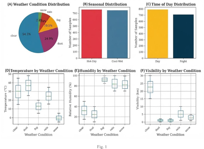
Figure 1: Characteristics of the synthetic dataset and environmental variables used for atmospheric attenuation modeling. (A) Distribution of meteorological conditions represented in the dataset, including clear-sky, dust, fog, rain, and snow situations. (B) Seasonal distribution of samples across hot-dry and cool-wet periods. (C) Distribution of samples collected during daytime and nighttime conditions. (D) Temperature distributions for each weather condition. (E) Humidity distributions for each weather condition. (F) Visibility distributions for each weather condition. Boxplots show the median (center line), interquartile range (box), and minimum and maximum values (whiskers). Temperature is reported in °C, humidity in %, and visibility in km. Please click here to view a larger version of this figure.

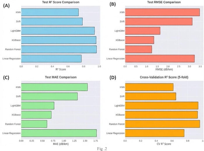
Figure 2: Performance comparison of machine learning models for atmospheric attenuation prediction. (A) Test coefficient of determination (R²) scores for the evaluated machine learning models, including Linear Regression, Random Forest, Extreme Gradient Boosting (XGBoost), Light Gradient Boosting Machine (LightGBM), Support Vector Regression (SVR), and K-Nearest Neighbors (KNN). (B) Test root mean square error (RMSE) values for each machine learning model. (C) Test mean absolute error (MAE) values for each machine learning model. (D) Cross-validation coefficient of determination (R²) scores obtained using five-fold cross-validation. Higher R² values and lower RMSE and MAE values indicate improved predictive performance. RMSE and MAE are reported in dB/km. Please click here to view a larger version of this figure.

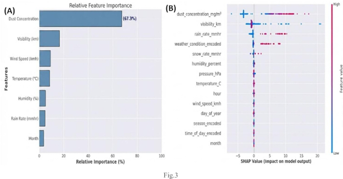
Figure 3: Feature importance and model interpretability analysis for atmospheric attenuation prediction. (A) Relative impurity-based feature importance rankings from the Random Forest model showing the contribution of all 10 environmental and temporal variables to attenuation prediction. The most influential feature was the dust concentration (67.3%) followed by visibility (21.2%), rain rate (6.0%), wind speed (2.1%), temperature (1.5%), humidity (0.9%), month (0.5%), season (0.3%), snowfall rate (0.1%), and atmospheric pressure (0.1%). The relative importance is a percentage of the total model importance. (B) SHapley Additive exPlanations (SHAP) summary plot illustrating the impact of individual features on model predictions. The SHAP matrix was computed for 300 test-set samples (300 × 10 features). For the one-hot-encoded season variable (originally four binary columns: spring, summer, autumn, winter), the SHAP values were combined by summing across the four categories to produce a single ‘season’ contribution value per sample. Each point represents a sample, and the color scale indicates the feature value, ranging from low (blue) to high (red). Positive SHAP values indicate an increase in the predicted attenuation, whereas negative SHAP values indicate a decrease in the predicted attenuation. Please click here to view a larger version of this figure.

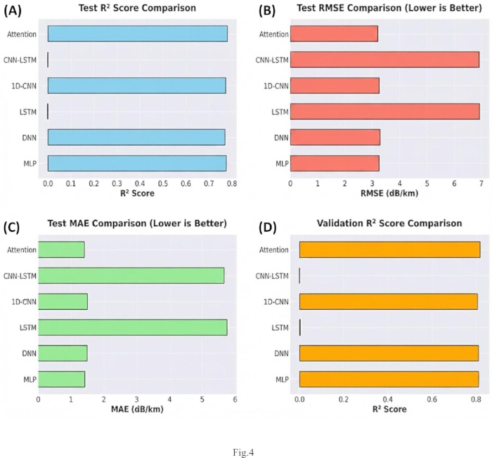
Figure 4: Performance comparison of deep learning models for atmospheric attenuation prediction. (A) Test coefficient of determination (R²) scores for the evaluated deep learning architectures, including Multilayer Perceptron (MLP), Deep Neural Network (DNN), Long Short-Term Memory (LSTM), one-dimensional convolutional neural network (1D-CNN), Convolutional Neural Network–Long Short-Term Memory (CNN–LSTM), and Attention-based models. (B) Test root mean square error (RMSE) values for each deep learning model. (C) Test mean absolute error (MAE) values for each deep learning model. (D) Validation coefficient of determination (R²) scores for the evaluated deep learning models. Higher R² values and lower RMSE and MAE values indicate improved predictive performance. RMSE and MAE are reported in dB/km. Please click here to view a larger version of this figure.

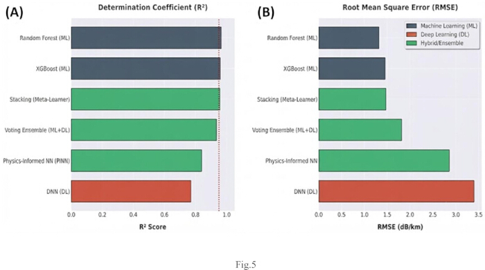
Figure 5: Comparative performance of machine learning, deep learning, and hybrid models for atmospheric attenuation prediction. (A) Coefficient of determination (R²) values for representative machine learning, deep learning, and hybrid approaches, including Random Forest, Extreme Gradient Boosting (XGBoost), Deep Neural Network (DNN), Voting Ensemble, Stacking, and Physics-Informed Neural Network models. (B) Root mean square error (RMSE) values for the same models. Machine learning (ML), deep learning (DL), and hybrid/ensemble techniques are the three categories into which models are color-coded. Improved predictive performance is indicated by higher R² and lower RMSE values. RMSE is expressed in dB/km. Please click here to view a larger version of this figure.

Weather Condition	Proportion	Temperature Range	Humidity Range	Visibility Range	Primary Parameter Range
Clear Sky	54.27% (814 samples)	−4.89 to 47.99°C	0–100%	>10 km	—
Dust	25.00% (375 samples)	10–45°C	10–60%	0.05–5 km	Dust: 0–4.96 mg/m3
Fog	10.47% (157 samples)	−5 to 20°C	70–100%	0.05–1 km	—
Rain	7.40% (111 samples)	5–30°C	60–100%	1–10 km	Rain: 0.25–50 mm/h
Snow	2.87% (43 samples)	−10 to 5°C	50–100%	0.5–5 km	Snow: 0.5–15 mm/h

Table 1: Machine learning models' performance measures for predicting atmospheric attenuation.

Model	Test R2	RMSE (dB/km)	MAE (dB/km)	CV R2	Training Time (s)
Random Forest	0.9654	1.324	0.815	0.960 ± 0.007	1.6
XGBoost	0.9582	1.455	0.892	0.953 ± 0.009	2.1
LightGBM	0.9507	1.581	0.971	0.946 ± 0.011	1.8
Support Vector Regression (SVR)	0.8874	2.389	1.445	0.879 ± 0.015	3.2
Linear Regression	0.8358	2.889	1.791	0.831 ± 0.018	0.2
K-Nearest Neighbors (KNN)	0.7341	3.671	2.296	0.721 ± 0.022	0.8

Table 2: Comparative evaluation of specific deep learning, hybrid, and machine learning models.

Model	Category	Test R2	RMSE (dB/km)	Rank
Random Forest	ML	0.9654	1.324	1
XGBoost	ML	0.9582	1.455	2
Stacking Ensemble	Hybrid	0.9571	1.473	3
LightGBM	ML	0.9507	1.581	4
Voting Ensemble	Hybrid	0.934	1.827	5
Physics-Informed Neural Network	Hybrid	0.8269	2.96	6
Attention	DL	0.7766	3.362	7
LSTM / CNN–LSTM	DL	−0.0006	7.195	—

Table 3: Comparison of each assessed model's efficiency in computation (training and inference).

DATA  AVAILABILITY:

The complete synthetic dataset of 1,500 samples with all input features (temperature, humidity, visibility, dust concentration, rainfall rate, snowfall rate, wind speed, atmospheric pressure, month, season, and weather condition) and target variable (attenuation in dB/km) is provided as a supplementary file along with this manuscript in https://doi.org/10.5281/zenodo.21792999. The data set is formatted so that each sample has one row, including all calculated variables (operating range and SNR).

The full implementation code, including: data generation scripts (implementations of physical models); functions for preprocessing and feature scaling; all implementations of machine learning models; all deep learning model implementations; scripts for evaluation and visualization; and hyperparameter tuning and cross-validation procedures, is also intended to be provided as a supplementary file.

Source Climate Data: The climate data used to define the synthetic-data distributions were obtained from the Iraqi Meteorological Organization and Seismology (IMOS) and the Iraqi Ministry of Transport, covering the period 2020–2024. A summary of the climate data used to determine the proportions of weather conditions and parameter ranges is provided in Supplementary Table 1. The specific IMOS records used in this study are not publicly archived in a centralized repository but can be requested directly from IMOS. The summary statistics and derived probability distributions are provided in the supplementary materials to enable reproducibility.

Repository Information: The source code and dataset are deposited in a public repository (Zenodo) with https://doi.org/10.5281/zenodo.21792999.

Discussion

In order to forecast air attenuation in FSO communication systems operating under Iraqi weather conditions, the current study assessed machine learning, deep learning, and hybrid techniques. Since atmospheric impacts continue to be one of the main issues affecting link performance and availability, recent evaluations have emphasized the increasing significance of predictive modelling for FSO systems²¹. The results showed that classical machine learning approaches, particularly RF and XGBoost, delivered high predictive accuracy and in some cases numerically outperformed deep learning and hybrid methods. However, statistical tests did not show a significant difference (p=0.083) between RF and the best hybrid ensemble (Stacking), which means that both approaches can reach similar results on this dataset. Our findings indicate that tree-based ensemble methods are still highly performant for tabular environmental data with moderate sample sizes and a small number of dominant predictor variables. Analysis of feature importance showed that dust concentration and visibility were the main drivers of attenuation, together explaining the majority of the predictive power. This finding agrees with earlier investigations showing the important influence of fog, dust, aerosols and atmospheric pollution on the propagation of the optical signal^22,23,24,25. Similar findings have been reported in environmental monitoring applications, where machine learning models often benefit from datasets containing a small number of highly informative variables^{26,27,28,29,30,31,32}. The SHAP analysis further improved model interpretability by quantifying the influence of individual environmental parameters on attenuation predictions.

The lower performance of deep learning models may be attributed to several factors. The dataset size was relatively modest for training complex neural architectures (in https://doi.org/10.5281/zenodo.21792999), and the environmental variables exhibited highly concentrated feature importance. Previous studies have shown that deep learning methods generally benefit from large datasets, hierarchical feature structures, and complex nonlinear representations^{33,34,35,36,37}. In contrast, the attenuation dataset used in this study contained a limited number of dominant predictors and lacked the temporal dependencies required for recurrent architectures. The poor performance of LSTM and CNN–LSTM models suggests that sequential learning mechanisms may not provide substantial benefits for this application.

The dominance of dust concentration (67.3%) and visibility (21.2%) as predictors of atmospheric attenuation may be attributed to several factors. First, the molecular scattering and absorption at 1550 nm are overshadowed by the Mie scattering from dust particles. In Mie theory, the extinction efficiency Q_ext is highly sensitive to particle concentration, and the attenuation scales almost linearly with dust concentration in the moderate-to-high concentration regime. Second, Iraq is subject to frequent dust storms (25.00% of days in our climate records), which result in attenuation values of 4–30 dB/km. This contrasts with fog (10.47%, 0.5–10 dB/km) and rain (7.40%, 2–25 dB/km). The greater variability in dust attenuation yields stronger signals for the models to learn from. Third, the dust concentration exponential distribution (0.4–4.96 mg/m³) produces a wide range of attenuation values. The long tail for extreme dust events yields high attenuation values, which are important for accurate prediction. Fourth, the Mie scattering model has a simpler (roughly linear) dependence on dust concentration, which is easier for tree-based models to approximate compared to the more complex relationship between visibility and fog attenuation in the Kim model. Fifth, this finding is of practical significance because dust storms are one of the most challenging environmental conditions for FSO in the Middle East. Accurate prediction during the dust events is essential for the reliable operation of the system.

The findings advance FSO communication research by providing practical guidance on algorithm selection for atmospheric attenuation prediction. Accurate attenuation forecasting is essential for network planning, adaptive link management, and reliable deployment of optical communication systems in challenging environments such as the Middle East^23,28,30,36. In addition, the methodology may be applicable to other environmental prediction problems involving air propagation, atmospheric monitoring, and optical network performance assessment^38,39,40. Larger real-world datasets, sophisticated ensemble learning techniques, transfer learning frameworks, or more complex physics-informed architectures are some other methods for examining this idea^{41,42,43,44,45}.

Scope of conclusions and generalizability issues

The conclusions of this work are mainly based on a synthetic dataset generated from well-established physical propagation models (Beer-Lambert law, Kim model, Carbonneau model, and Mie scattering theory). This methodological approach carries some implications for the scope and generalization of our findings:

Conclusions From Simulated Data: (1) Comparative performance ranking of machine learning, deep learning, and hybrid approaches for atmospheric attenuation prediction. (2) Identification of dust concentration and visibility as the dominant environmental predictors of optical attenuation under the modeled conditions. (3) Computational efficiency advantage of tree-based ensemble methods over deep learning architectures. (4) Interpretability of feature importance and SHAP analyses to explain model predictions.

Conclusions Requiring Real-World Confirmation: (1) The absolute values of R² and RMSE obtained by the evaluated models are dependent on the specific characteristics of the synthetic dataset and may reflect the models' learning the deterministic physical equations used to generate the targets. (2) It is yet to be proven that the best model, Random Forest, can be applied to unknown real-world atmospheric conditions. (3) Field validation is necessary for the findings to be applicable to operational FSO units installed in Iraq. (4) It is necessary to confirm that the identified feature importance rankings are resilient under field measurement conditions.

It is important to distinguish between performance on equation-derived synthetic data and performance on noisy observational or experimental data. The synthetic dataset provides a clean noise free relationship between input features and the attenuation target, which may produce higher predictive performance indicators than what can be obtained with real-world data with measurement noise, instrument errors and unmodeled physical phenomena. We recommend that future work be directed toward obtaining real world FSO attenuation measurements under the Iraqi weather conditions, to validate the results presented in this study and to assess the true generalizability of the proposed methodologies.

Implications of synthetic data for model generalizability

The implications of using synthetic data in this study should be carefully considered for the generalizability of the models:

Advantages of the Synthetic Approach The dataset is physically consistent and based on established theoretical frameworks through the use of established physical propagation models. Meteorological parameters were extracted from meteorological records of Iraq to make the dataset reflect the statistical properties of the real weather conditions in Iraq. In addition to avoiding the confounding variables of field measurements (such as measurement errors, equipment calibration, or insufficient data records), this controlled setting enables a methodical examination of modeling methodologies.

Limitations to Generalizability The synthetic dataset has limitations in capturing the full complexity of real atmospheric attenuation including: (1) the interaction of multiple atmospheric phenomena happening at the same time; (2) non-linear and non-stationary behavior of atmospheric parameters; (3) long-term climate variability not captured by the sampling distributions; (4) localized microclimatic effects that may significantly affect FSO propagation; and (5) noise and uncertainty inherent in real-world data collection.

Bias considerations in synthetic data generation The assumption of independent sampling of environmental parameters (see Methods) is an oversimplification of real-world conditions, where atmospheric variables tend to be correlated (e.g., high dust concentrations tend to be correlated with low visibility). An independence assumption was made for a controlled simulation environment for systematic model comparison. However, this method may not capture the full complexity of the interactions of atmospheric parameters. We employ a stratified splitting method (maintaining the ratios of weather conditions in the training and testing sets) to minimize the chance of an unbalanced representation of rare conditions in the testing set (notably snow at 2.87%).

Deterministic Target Generation: The high predictive performance observed in this study may be partially explained by the models learning the deterministic physical equations used to generate the target values. In contrast, real-world experimental data contain measurement noise, instrument errors, and unmodeled physical phenomena that make prediction more challenging. Therefore, the quantitative performance metrics (R², RMSE, MAE) should be interpreted as relative comparisons between methodologies in a controlled simulation environment, rather than as absolute performance guarantees for operational FSO systems.

Therefore, while the comparative results on model performance rankings are likely robust (due to the physical consistency of the synthetic data), the absolute performance metrics (R², RMSE, MAE) should not be taken as indicative of expected performance in operational FSO systems. It is necessary to test the model's generalizability to real-world settings using experimental air attenuation measurements obtained under various weather conditions in Iraq.

There are a few restrictions to be aware of. First, rather of using field observations, the study relied on a synthetic dataset produced using well-known physical propagation models. As previously said, rather than providing absolute performance guaranties for operational FSO systems, the quantitative performance metrics (R2, RMSE, MAE) should be viewed as relative comparisons of approaches in a controlled simulation environment. Second, standard versus deep learning models may not have been able to learn robust feature representations due to the magnitude of the dataset. Third, other FSO performance indicators like connection availability, pointing faults, and turbulence-induced fading were not taken into account in favor of attenuation prediction. Fourth, historical records from 2020 to 2024 were used to calculate the proportions of weather conditions, which might not accurately reflect variations in Iraqi climatic patterns from year to year. Fifth, the pseudo-sequential input data structure of the CNN–LSTM and LSTM models is a methodological simplification that may not adequately capture the temporal dynamics of real-world applications. When evaluating the results, these limitations should be taken into account as they may have an impact on the findings' generalizability.
Recommended Priority: Verification in the Actual World Gathering and analyzing actual FSO attenuation measurements under Iraqi weather conditions is the most crucial future work path. This should involve: (1) setting up FSO testbeds in various parts of Iraq (e.g., Baghdad, Basra, Mosul, Ramadi) to record regional climate variations; (2) using calibrated instruments at FSO locations to simultaneously measure atmospheric parameters (temperature, humidity, visibility, dust concentration); (4) documenting the attenuation during extreme weather events (dust storms, heavy fog, heavy rain); (5) making the collected data publicly available to enable reproducibility and comparative research; and (3) continuing monitoring for at least one complete annual cycle to capture the seasonal fluctuation. Such practical validation would offer a chance to assess the generalizability of the model and enhance the predictive techniques created in this research.

To validate and enhance the generated models, future research should focus on incorporating actual FSO measurements obtained in Iraqi weather conditions. Additional research could examine transfer learning strategies that make use of relevant atmospheric datasets, online learning programs that adjust to shifting environmental conditions, and hybrid experimental–simulation strategies that combine measured data with physical models. Additional research into explainable AI and sophisticated physics-based learning approaches may also shed more light on the mechanisms underlying air attenuation and strengthen the resilience of upcoming prediction systems.

Materials

List of materials used in this article

Name	Company	Catalog Number	Comments
CUDA Toolkit	NVIDIA Corporation	11.8	GPU-acceleration library for deep learning training
cuDNN	NVIDIA Corporation	8.6.0	GPU-accelerated deep neural network library
GPU (graphics processing unit)	NVIDIA Corporation	GeForce RTX 4090, 24 GB VRAM	Used for GPU-accelerated deep learning training
CPU (central processing unit)	Intel Corporation	Core i9-13900K, 24 cores/32 threads	Workstation processor for all model training/evaluation
System memory (RAM)	n/a	64 GB DDR5, 5200 MHz	Workstation memory
Keras API	Open source (part of TensorFlow)	bundled with TensorFlow 2.11.0	High-level deep learning API used for all DL architectures
LightGBM	Open source (Microsoft)	3.3.5	Gradient boosting framework
NumPy	Open source (NumFOCUS)	1.23.5	Numerical computation library
Operating system	Canonical Ltd.	Ubuntu 22.04 LTS	Workstation operating system
Python	Python Software Foundation	3.9	Programming language used for all data generation and modeling
scikit-learn	Open source	1.2.2	Machine learning library (RF, SVR, KNN, Linear Regression, cross-validation, scaling)
SHAP (SHapley Additive exPlanations)	Open source	0.41.0	Model interpretability library, TreeExplainer module
TensorFlow	Open source (Google)	2.11.0	Deep learning framework used for all six DL architectures
XGBoost	Open source	1.7.5	Extreme Gradient Boosting library

References

- Kadhim MS, Hussein H, Elwi TA. Hybrid ANN-Z method for modeling carbon nanotube-based reconfigurable intelligent surfaces for terahertz beam steering. J Vis Exp. 2026;in press.
- Raham JK, Alshaibi M, Elwi TA. SMS optical fiber laser sensor for transformer oil temperature monitoring-based IoT of AI control. Prog Electromagn Res B. 2026;118:72–86.
- Abdulkareem ZJ, Hamad TK, Elwi TA. Reconfigurable metasurface based on graphene optical antennas for dynamic beam steering. Sustain Eng Innov. 2025;7:127–136.
- Abdulsattar RK, et al. Optical-microwave sensor for real-time measurement of water contamination in oil derivatives. AEU Int J Electron Commun. 2023;170:154798. doi:10.1016/j.aeue.2023.154798.
- Al-Khaylani HH, Elwi TA, Ibrahim AA. Optically remote control of miniaturized 3D reconfigurable CRLH printed self-powered MIMO antenna array for 5G applications. Micromachines. 2022;13(12):2061. doi:10.3390/mi13122061.
- Al-Khaylani HH, Elwi TA, Ibrahim AA. Optically remote-controlled miniaturized 3D reconfigurable CRLH-printed MIMO antenna array for 5G applications. Microw Opt Technol Lett. 2023;65(2):603–610.
- Jassim DA, Elwi TA. Optical nano monopoles for interconnection of electronic chip applications. Optik. 2022;249:168142. doi:10.1016/j.ijleo.2021.168142.
- Elwi TA. A novel approach for modeling the geometry and constitutive parameters of an armchair single-wall carbon nanotube antenna operating in the NIR regime. Al-Ma’mon Coll J. 2014;(24):261–285.
- Mohammed, AB.F.A., Al-hadeethi, S.T., Al-khaylani, H.H. et al. An investigation of success probability and fidelity of quantum repeater in asymmetry in midpoint placement in fiber-based quantum networks. J Opt (2025). https://doi.org/10.1007/s12596-025-02866-6.
- Kim II, McArthur B, Korevaar EJ. Comparison of laser beam propagation at 785 nm and 1550 nm in fog and haze for optical wireless communications [conference paper]. Presented at: Optical Wireless Communications III; Boston, MA, USA; 2000. Proc SPIE. 2001;4214:26–37. https://doi.org/10.1117/12.417512.
- Okbi ZA, Alak IK, Abdulla EN, Al-Khaylani HH. Design and security analysis of an image encryption based on a gigabit passive optical network employing fiber-FSO protection at the last mile. J Opt Commun. 2025. doi:10.1515/joc-2025-0466.
- Ojo JS, Olaitan JA, Ojo OL. Characterization of fog-induced attenuation for optimizing optical propagation links in Nigeria. Results Opt. 2022;9:100279. doi:10.1016/j.rio.2022.100279.
- Khidher SA. Dust storms in Iraq: Past and present. Theor Appl Climatol. 2024;155:4721–4735.
- Ali, Alaa Hussein, Abdulla, Essam N. and Al-Azawi, Razi J.. "Security and network performance analysis of coexistence TWDM – NG-PON2, GPON and 10G-EPON systems based on Hill Cipher" Journal of Optical Communications, 2025. https://doi.org/10.1515/joc-2025-0435.
- Lionis A, et al. Using machine learning algorithms for accurate received optical power prediction of an FSO link over a maritime environment. Photonics. 2021;8(6):212. doi:10.3390/photonics8060212.
- Chen T, Guestrin C. XGBoost: A scalable tree boosting system [conference paper]. Presented at: 22nd ACM SIGKDD International Conference on Knowledge Discovery and Data Mining; San Francisco, CA, USA; 2016. p. 785–794. https://doi.org/10.1145/2939672.2939785.
- Bai Y, et al. Air pollutants concentrations forecasting using back propagation neural network based on wavelet decomposition with meteorological conditions. Atmos Pollut Res. 2016;7(3):557–566.
- LeCun Y, Bengio Y, Hinton G. Deep learning. Nature. 2015;521:436–444.
- Mousa, Ekhlass, Abdulla, Essam N. and Adnan, Salah A.. "Enhancing network security based on 10G-EPON with the use of the Hill cipher algorithm" Journal of Optical Communications, 2025. https://doi.org/10.1515/joc-2025-0201.
- Lu G, et al. A survey of deep learning for time series forecasting: Theories, datasets, and state-of-the-art techniques. Comput Mater Contin. 2025;85(2):2403–2441.
- Liu J, Yang X, Wei Y, Zhao F. Integrated THz/FSO communications: A review of practical constraints, applications and challenges. Micromachines. 2025;16(11):1297. doi:10.3390/mi16111297.
- Bott A, Sievers U, Zdunkowski W. A radiation fog model with a detailed treatment of the interaction between radiative transfer and fog microphysics. J Atmos Sci. 1990;47:2153–2166.
- Fadhil HA, et al. Optimization of free space optics parameters: An optimum solution for bad weather conditions. Optik. 2013;124(19):3969–3973.
- Osipov S, et al. Severe atmospheric pollution in the Middle East is attributable to anthropogenic sources. Commun Earth Environ. 2022;3:203. doi:10.1038/s43247-022-00514-6.
- Castellanos P, et al. Mineral dust optical properties for remote sensing and global modeling: A review. Remote Sens Environ. 2024;303:113982. doi:10.1016/j.rse.2023.113982.
- Lolli S. Urban PM2.5 concentration monitoring: A review of recent advances in ground-based, satellite, model, and machine learning integration. Urban Clim. 2025;63:102566. doi:10.1016/j.uclim.2025.102566.
- Ridha, Fay F., Abdulla, Essam N. and Abdulhadi, Ali H.. "Machine learning based on raw ensemble predictions scheme for TWDM-PON" Journal of Optical Communications, 2025. https://doi.org/10.1515/joc-2025-0373.
- Khalid H, Sajid SM, Cheema MI, Leitgeb E. Optical signal attenuation through smog in controlled laboratory conditions. Photonics. 2024;11(2):172. doi:10.3390/photonics11020172.
- Ejike O, Ndị D, Shakir MZ. Comparative study of machine learning-based rainfall prediction in tropical and temperate climates. Climate. 2025;13(8):167. doi:10.3390/cli13080167.
- Esmail MA, Fathallah H, Alouini MS. An experimental study of FSO link performance in desert environment. IEEE Commun Lett. 2016;20(9):1888–1891.
- Kshirsagar MP, Khare KC. Support vector regression models of stormwater quality for a mixed urban land use. Hydrology. 2023;10(3):66. doi:10.3390/hydrology10030066.
- Mosso S, Lapo K, Stiperski I. Revealing the drivers of turbulence anisotropy over flat and complex terrain: An interpretable machine learning approach. Boundary Layer Meteorol. 2025;191:51. doi:10.1007/s10546-025-00946-5.
- Mohsen S, Ali AM, Emam A. Automatic modulation recognition using CNN deep learning models. Multimed Tools Appl. 2024;83:7035–7056.
- Mienye ID, Swart TG, Obaido G. Recurrent neural networks: A comprehensive review of architectures, variants, and applications. Information. 2024;15(9):517. doi:10.3390/info15090517.
- Castelli M, et al. Generative adversarial networks for generating synthetic features for Wi-Fi signal quality. PLoS One. 2021;16(11). doi:10.1371/journal.pone.0260308.
- Al-Imran, Chowdhury MZ, Mofidul RB, Jang YM. Machine learning and deep learning in FSO communication: A comprehensive survey. ICT Express. 2025;11(6):1026–1046.
- Grose MG, Watson EA. Forecasting atmospheric turbulence conditions from prior environmental parameters using artificial neural networks. Appl Opt. 2023;62:3370–3379.
- Radhi SS, et al. Design a secure TWDM-PON via the Hill cipher algorithm. Opt Contin. 2025;4:1051–1064.
- Mushatet, Adil Fadhil, Fadil, Elaf A. and Abdulla, Essam N.. "High bit rate secure FSO system utilizing Hill coding" Journal of Optical Communications, 2025. https://doi.org/10.1515/joc-2025-0147.
- Musadaq R, Abdulwahid SN, Abd Alwahed NN, Abdulla EN. Security analysis of an image encryption algorithm based on Blowfish in GPON. J Opt Commun. 2025. doi:10.1515/joc-2025-0109.
- Raissi M, Yazdani A, Karniadakis GE. Hidden fluid mechanics: Learning velocity and pressure fields from flow visualizations. Science. 2020;367(6481):1026–1030.
- Vasiliauskaite V, Antulov-Fantulin N. Generalization of neural network models for complex network dynamics. Commun Phys. 2024;7:348. doi:10.1038/s42005-024-01837-w.
- Oh S, Hong SK. Physics-informed neural modeling of 2D transient electromagnetic fields. Appl Sci. 2025;15(23):12612. doi:10.3390/app152312612.
- Pradhan S, Bhattarai JS, Murugavel M, Sharma OP. Machine learning approaches to surpass the limitations of the Beer–Lambert law. ACS Omega. 2025;10(16):16597–16601.
- Pavlyshenko B. Using stacking approaches for machine learning models [conference paper]. Presented at: 2018 IEEE Second International Conference on Data Stream Mining and Processing (DSMP); Lviv, Ukraine; 2018. p. 255–258. https://doi.org/10.1109/DSMP.2018.8478522.