This protocol presents a reproducible workflow for multi-scenario land-use projection, carbon storage assessment, and topographic association analysis in the Yixian–Huangshan World Heritage landscape.
Method Article
Multi-Scenario Land-Use Projection and Carbon Storage Assessment in the Yixian-Huangshan World Heritage Landscape
In This Article
Summary
Abstract
Land-use change alters terrestrial carbon storage, yet reproducible workflows for evaluating scenario-based changes remain limited in tourism-oriented World Heritage landscapes. This protocol integrates a custom Markov cellular automaton, four-pool carbon accounting equivalent to the Integrated Valuation of Ecosystem Services and Tradeoffs framework, and an optimal parameters-based geographical detector to assess land-use and carbon-storage changes across Yixian and adjacent areas of Huangshan in southern Anhui, China. China Land Cover Dataset maps from 2005, 2010, and 2015 were used for calibration and out-of-period validation. Four exploratory scenarios—Business As Usual, Tourism Expansion and Development, Ecological Conservation Priority, and Village Revitalization and Activation—were simulated for 2030 and 2050. Validation across 4,632,329 valid pixels yielded an overall accuracy of 96.61%, a Kappa coefficient of 0.850, and a Figure of Merit of 0.107. Baseline carbon storage was 59.505 teragrams of carbon, with forests contributing 95.9%. Projected carbon losses by 2050 ranged from 5.01% under Ecological Conservation Priority to 13.49% under Tourism Expansion and Development. Matched one-at-a-time perturbations supported the same scenario ordering. The optimal parameters-based geographical detector identified slope, relief, and elevation as the strongest assessed topographic associations. The supplied inputs, parameters, outputs, and scripts support reproducibility; however, the scenarios should be interpreted as comparative stress tests rather than calibrated forecasts.
Introduction
Terrestrial ecosystems store carbon in vegetation, soil, and dead organic matter, thereby contributing to climate regulation1,2. Land conversion can rapidly alter these stocks; spatially explicit assessment is therefore important for land-use planning and carbon management.
The analytical extent in southern Anhui encompasses extensive subtropical forests, agricultural basins, and areas associated with the Mount Huangshan and Xidi–Hongcun World Heritage properties3,4. Research on cultural-heritage land cover, World Heritage tourism, and traditional-village conservation indicates that ecological condition, visitor pressure, and place identity require integrated consideration in this setting5,6,7.
Scenario-based land-use models translate observed transitions into spatially explicit projections, and carbon-pool accounting quantifies the consequences of those patterns. Previous studies have combined Patch-generating Land Use Simulation (PLUS) or cellular automaton–Markov (CA–Markov) allocation with the Integrated Valuation of Ecosystem Services and Tradeoffs (InVEST) framework and the optimal parameters-based geographical detector (OPGD) in China and other landscapes, including recent integrated applications8,9,10,11,12,13,14,15,16,17,18,19,20. These studies provide methodological precedents, although the simulator used here is a custom Markov cellular automaton (Markov-CA) implementation rather than PLUS.
Related research has evaluated policy-conditioned carbon trajectories, coupled satellite and land-use models, terrain-sensitive carbon storage, urban and campus applications, soil-carbon management, cropland transitions, national forest mapping, and scale dependence21,22,23,24,25,26,27,28,29,30,31,32,33,34. Collectively, these studies support multi-scenario comparison while demonstrating that conclusions depend on data scale, class transitions, carbon parameters, and modeled policy assumptions. The custom implementation used in the present study provides a transparent workflow in which the transition matrix, scenario multipliers, allocation procedure, carbon-density lookup, sensitivity analysis, and topographic association analysis can be examined within a single reproducible framework. In the present study, the practical value of the custom workflow is that the transition matrix, scenario parameters, pixel-allocation rules, validation, sensitivity analysis, carbon accounting, and topographic association analysis are implemented and documented within a reproducible computational framework. This structure allows the assumptions and intermediate analytical steps used in the scenario analysis to be inspected and reproduced. Because the workflow was not benchmarked directly against PLUS or other CA–Markov implementations, no claim of superior accuracy, efficiency, or predictive performance is made.
Research on topographic and edaphic controls, geomorphic soil-carbon persistence, spatial-scale effects, OPGD applications, Huangshan productivity, landscape metrics, wetlands, and forest carbon further supports a cautious, association-based interpretation of terrain effects35,36,37,38,39,40,41,42,43,44. Against this background, the overall goal of the present method is to provide a transparent and reproducible workflow for multi-scenario land-use projection, carbon-storage assessment, and topographic association analysis in the Yixian–Huangshan World Heritage landscape. The workflow uses a custom Markov-CA implementation with InVEST-equivalent four-pool carbon accounting and OPGD, validates the model out of period for 2005–2015, and conducts a 28-run one-at-a-time sensitivity analysis. The accompanying rasters, scenario rules, confusion matrix, environment files, and scripts permit direct inspection and reproduction of the custom simulation workflow. The workflow is intended for applications with compatible categorical land-cover rasters, class-specific carbon-density parameters, and appropriate topographic data, where the objective is comparative scenario assessment rather than precise spatial forecasting.
This study had three objectives: (1) simulate land use for 2030 and 2050 under Business As Usual (BAU), Tourism Expansion and Development (TED), Ecological Conservation Priority (ECP), and Village Revitalization and Activation (VRA) stress tests; (2) quantify carbon storage using a complete nine-class, four-pool lookup; and (3) assess the individual and joint associations of elevation, slope, northness, and topographic relief with 2015 carbon density8,9,10. These objectives integrate land-use projection, carbon accounting, and terrain-association analysis within a single reproducible workflow while retaining the distinction between simulated land-use outcomes and statistical associations with topographic variables.
The scenario labels denote comparative assumptions rather than fitted forecasts or encoded statutory plans. Accordingly, the method is most appropriate for reproducible comparison of alternative land-use assumptions and their associated carbon-storage outcomes, rather than for interpreting the resulting maps as calibrated predictions of future land use.
Protocol
No human participants, animals, or protected species were involved. The analysis used only publicly available remote-sensing products and published carbon-density parameters; therefore, ethics committee approval was not required.
Implement all computational procedures in Python 3.11 within an open and reproducible workflow. Follow seven sections: (1) define the study area; (2) acquire and preprocess the inputs; (3) estimate the transition matrix and initialize the custom Markov-CA; (4) configure the scenarios, sensitivity tests, and future simulations; (5) calibrate and validate the model; (6) calculate carbon storage; and (7) detect terrain associations with OPGD. Follow the complete workflow shown in Figure 1.
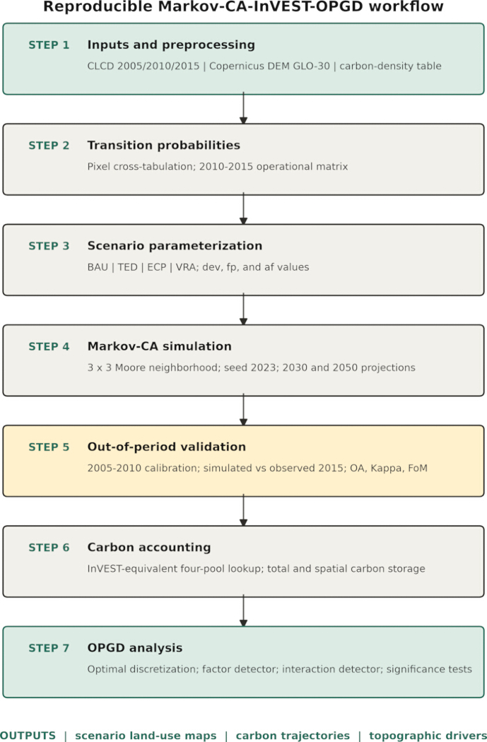
Figure 1. Reproducible workflow for multi-scenario land-use projection, carbon storage assessment, and topographic association analysis. The seven-step workflow comprises (1) input preparation and preprocessing using China Land Cover Dataset (CLCD) maps, Copernicus Digital Elevation Model (DEM) GLO-30 data, and the carbon-density table; (2) estimation of transition probabilities by pixel cross-tabulation; (3) parameterization of the Business As Usual (BAU), Tourism Expansion and Development (TED), Ecological Conservation Priority (ECP), and Village Revitalization and Activation (VRA) scenarios; (4) Markov cellular automaton (Markov-CA) simulation using a 3 × 3 Moore neighborhood; (5) out-of-period validation using overall accuracy (OA), Kappa, and Figure of Merit (FoM); (6) carbon accounting using an Integrated Valuation of Ecosystem Services and Tradeoffs (InVEST)-equivalent four-pool lookup; and (7) optimal parameters-based geographical detector (OPGD) analysis. The workflow produces scenario-specific land-use maps, carbon-storage trajectories, and assessments of topographic associations. Please click here to view a larger version of this figure.
1. Study area
- Define the analysis grid as 117.60–118.38°E and 29.72–30.22°N. Treat the Mount Huangshan and Xidi–Hongcun World Heritage properties as geographical context only; do not interpret the rectangular analytical extent or valid mask as an official administrative or World Heritage boundary3,4.
- Reproject the grid to EPSG:32650 and apply the valid mask to obtain 4,632,329 cells at 30 m resolution, representing 4,169.1 km2. Use this extent, which covers Yixian County, adjacent parts of the Huangshan Scenic Area, and northern Xiuning County, for all raster analyses (Figure 2).
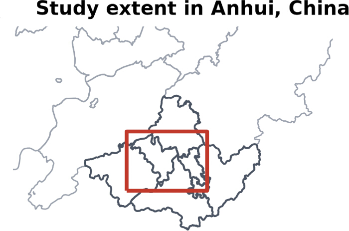
Figure 2. Study extent of the Yixian–Huangshan landscape in southern Anhui, China. Location of the analytical extent within Anhui Province, China, with the study area indicated by the red rectangle. The topographic variables used in the association analysis are presented in Figure 5. Please click here to view a larger version of this figure.
2. Data sources
- Use three input groups: CLCD annual land-cover data, Copernicus DEM GLO-30 terrain data, and a class-specific four-pool carbon-density table. Record the temporal coverage, resolution, provenance, and analytical role of each input in Table 1.
- Extract the 2005, 2010, and 2015 CLCD layers at 30 m resolution. Retain the nine classes: cropland, forest, shrub, grassland, water, snow/ice, barren, impervious, and wetland45.
- Derive elevation, slope, northness, and topographic relief from Copernicus DEM GLO-3046. Assign the complete nine-class carbon-pool values reported in Table 6 of Cheng et al.; do not apply an uncited default or zero-value convention47.
- Reproject all layers to WGS 84 / UTM zone 50N (EPSG:32650) on the common 30 m grid. Use nearest-neighbor resampling for categorical land cover and bilinear resampling for continuous terrain data.
- Apply the same valid mask to every layer before cross-tabulation, validation, carbon accounting, and OPGD sampling.
- Use Python 3.11.9 with numpy 2.4.6, scipy 1.17.1, rasterio 1.4.4, matplotlib 3.11.0, pandas 3.0.3, geopandas 1.1.4, and shapely 2.1.2. Refer to the archived environment files and relative-path scripts for exact reproduction.
- Configure the Markov-CA with a 3 × 3 Moore neighborhood and seed 2023. Initialize an independent seeded generator for each scenario-year and sensitivity run, and use seed 42 for OPGD sampling.
| Dataset | Temporal coverage | Native spatial resolution | Primary source / persistent identifier | Role in the analytical workflow |
| China Land Cover Dataset (CLCD; Yang & Huang45) | 2005, 2010, and 2015 | 30 m | Zenodo DOI: 10.5281/zenodo.4417810 | Land-use classification, change detection, validation, transition-matrix estimation, observed baseline, and Markov cellular automaton input |
| Copernicus Digital Elevation Model (DEM) GLO-30 | 2019 reference epoch; static in this study | 30 m | Copernicus Data Space Ecosystem / Microsoft Planetary Computer STAC | Elevation and derivation of slope, northness, and topographic relief using a 450 m-radius neighborhood |
| Carbon-density parameters | Static | Per land-use class; class lookup (Mg C ha⁻¹) | Cheng et al.47 Table 6 | Complete nine-class, four-pool lookup used for Integrated Valuation of Ecosystem Services and Tradeoffs-equivalent carbon accounting (Table 3) |
| Study-area analysis extent and boundary | Static | Vector / 30 m mask | Reconstructed from the manuscript extent: 117.60–118.38°E, 29.72–30.22°N; archived GeoJSON and mask | Common spatial mask, analysis extent, and analysis grid |
Table 1: Primary spatial and tabular datasets used in the analytical workflow. The table summarizes the temporal coverage, native spatial resolution, source or persistent identifier, and analytical role of the China Land Cover Dataset (CLCD), Copernicus Digital Elevation Model (DEM) GLO-30, class-specific carbon-density parameters, and study-area analysis extent. Carbon-density values are expressed in megagrams of carbon per hectare (Mg C ha−1).
3. Estimate the transition matrix and initialize the Markov-CA model
- Cross-tabulate valid CLCD pixels from 2010 to 2015. For source class i and target class j, calculate .
- Use the resulting 9 × 9 transition matrix for future scenarios. Derive a separate 2005–2010 transition matrix for model validation.
- Run the simulator as a custom Python Markov-CA implementation; do not invoke PLUS8.
- At each five-year step, take a synchronous snapshot of the starting state. Compute the transition counts from that snapshot.
- Evaluate target classes 1–9 and source classes 1–9 in ascending order. Remove each selected source pixel from further allocation so that it can transition at most once during the five-year step.
- Rank eligible candidate pixels by the start-of-step count of target-class neighbors in a 3 × 3 Moore window plus uniform random jitter from 0 to 0.5.
- Calculate the requested number of pixels for each source-to-target transition as the rounded product of the number of valid pixels in the source class, the corresponding transition probability, and the applicable scaling factor.
- Use a scaling factor of dev for transitions to impervious land and dev × fp for forest-to-impervious transitions; otherwise, use a scaling factor of 1. Cap the requested count at the number of eligible candidate pixels.
- If the requested count is smaller than the eligible candidate count, select the highest-ranked candidates based on the target-class neighborhood score plus the uniform random jitter described above; if the requested count equals the eligible candidate count, select all eligible candidates.
4. Configure scenarios, sensitivity tests, and future simulations
- Apply three parameters to the common transition matrix. Let dev scale expected transitions to impervious class 8, apply fp only to forest-to-impervious transitions, and define af as the per-step probability that cropland without an impervious Moore neighbor converts to forest.
- Set (dev, fp, af) to (1.4, 1.0, 0.005) for BAU, (6.0, 2.0, 0.001) for TED, (0.4, 0.4, 0.025) for ECP, and (2.5, 0.7, 0.012) for VRA. Use Table 2 for the corresponding computational rules, policy narratives, and parameter values.
- Interpret the multipliers as transparent low-, intermediate-, and high-development stress tests around the empirical transition matrix. Do not treat them as coefficients estimated from tourism, village-node, zoning, transport, protected-area, or ecological-redline data.
- Use the policy labels only to describe relative parameter directions. Do not interpret the labels as legal or spatial constraints encoded in the model.
- Treat dev, fp, and af as author-defined exploratory stress-test parameters rather than empirically estimated or calibrated coefficients. The nominal values specify contrasting numerical scenario assumptions for development pressure (dev), forest protection (fp), and afforestation (af); they were not fitted to observed post-2015 land-use change or interpreted as estimates of specific policy effects. Use these nominal values for the primary scenario comparisons and evaluate their robustness using the one-at-a-time sensitivity analysis described below.
- For each scenario, run the nominal 2050 case. Repeat the simulation after multiplying one of dev, fp, or af by 0.5 or 1.5 while holding the other parameters constant.
- Reinitialize seed 2023 for each of the 28 runs. Compare carbon storage, carbon loss, forest share, and impervious share, and report matched-case rankings and the full OAT ranges without treating them as probabilistic confidence intervals.
- Initialize every future simulation from observed CLCD 2015. For impervious allocation, allow cropland to remain eligible across the valid mask and require non-cropland source pixels to border start-of-step impervious cells.
- After class-to-class allocation, convert qualifying cropland to forest independently with probability af. Run three five-year steps for the 2030 projection and seven five-year steps for the 2050 projection.
- Preserve class 0 outside the valid mask. Export every projected map at 30 m resolution.
| Scenario | Implemented computational rule | Policy narrative (not an encoded constraint) | Parameters (dev / fp / af) |
| Business As Usual (BAU) | Moderate impervious multiplier; baseline forest susceptibility; 0.5% isolated-cropland afforestation per step | Continuation benchmark | 1.4 / 1.0 / 0.005 |
| Tourism Expansion and Development (TED) | Strong impervious multiplier; doubled forest-to-impervious susceptibility; weak afforestation | High-development stress test | 6.0 / 2.0 / 0.001 |
| Ecological Conservation Priority (ECP) | Reduced impervious conversion and forest susceptibility; strongest afforestation | Ecological-conservation stress test | 0.4 / 0.4 / 0.025 |
| Village Revitalization and Activation (VRA) | Intermediate impervious multiplier; forest susceptibility below BAU; intermediate afforestation | Village-revitalization narrative; no village-node layer | 2.5 / 0.7 / 0.012 |
Table 2: Computational rules and parameter values for the four land-use scenarios. The table summarizes the implemented computational rules, policy narratives, and parameter values for the Business As Usual (BAU), Tourism Expansion and Development (TED), Ecological Conservation Priority (ECP), and Village Revitalization and Activation (VRA) scenarios. Policy narratives describe the intended interpretation of each scenario and are not encoded spatial constraints. dev, impervious-development multiplier; fp, forest-to-impervious susceptibility multiplier; af, isolated-cropland afforestation fraction per simulation step.
5. Calibrate and validate the land-use model
- Estimate the calibration matrix from observed 2005–2010 change. Simulate 2015 from observed 2010 using seed 2023.
- Compare the simulated 2015 map pixel by pixel with observed CLCD 2015 within the valid mask. Calculate overall accuracy, Kappa, the 9 × 9 confusion matrix, and FoM for changed cells48.
- Exclude invalid cells from both the numerator and denominator of the validation calculations to prevent outside-mask zeros from inflating agreement.
- Interpret overall accuracy and Kappa jointly with FoM because stable forest and cropland dominate the former metrics, whereas FoM evaluates the smaller changed-cell set. Use the validation results to support regional scenario comparison; do not interpret them as establishing precise change-location forecasting.
6. Calculate carbon storage
- For each valid pixel, assign the four class-specific carbon-pool densities listed in Table 3. Sum the four pool densities to obtain the total carbon density in Mg C ha⁻1.
- Multiply the total carbon density by the 0.09 ha pixel area. Convert the resulting Mg C values to Tg C.
- Apply this lookup calculation as the algebraic equivalent of the InVEST Carbon Storage formulation. Do not apply a sequestration-rate, valuation, or economic module9,47.
| Land-use class (CLCD) | Aboveground C (Mg C ha⁻¹) | Belowground C (Mg C ha⁻¹) | Soil C (Mg C ha⁻¹) | Dead organic C (Mg C ha⁻¹) | Total C (Mg C ha⁻¹) | Source |
| 1 Cropland | 3.56 | 7.45 | 26.9 | 9.82 | 47.73 | Cheng et al.47, Table 6 |
| 2 Forest | 53.59 | 17.36 | 84.85 | 2.8 | 158.6 | |
| 3 Shrub | 4.25 | 4.65 | 72.9 | 1.59 | 83.39 | |
| 4 Grassland | 4.15 | 16.58 | 78.2 | 1.55 | 100.48 | |
| 5 Water | 6.38 | 0 | 0 | 0.12 | 6.5 | |
| 6 Snow/ice | 0 | 0.33 | 5.35 | 0 | 5.68 | |
| 7 Barren | 1.3 | 0.33 | 21.6 | 0 | 23.23 | |
| 8 Impervious | 0 | 0 | 9.28 | 0 | 9.28 | |
| 9 Wetland | 12.24 | 9.18 | 95.73 | 4.08 | 121.23 |
Table 3: Carbon-density parameters for the nine China Land Cover Dataset land-use classes used in carbon accounting. Aboveground, belowground, soil, dead organic, and total carbon-density values are provided for each China Land Cover Dataset (CLCD) land-use class. Total carbon density represents the sum of the four carbon pools. All carbon-density values are expressed in megagrams of carbon per hectare (Mg C ha−1). Values were obtained from Cheng et al.47, Table 6.
7. Detect topographic associations with OPGD
- Use 2015 carbon density as the response variable and elevation, slope, northness, and topographic relief as the explanatory factors. Sample 200,000 valid pixels using seed 42.
- For each explanatory factor, test 2–15 quantile intervals. Retain the discretization that produces the maximum q-value.
- Calculate analytic F-test p-values and permutation p-values using 999 permutations. Calculate the permutation p-value as p = (exceedances + 1) / 1000.
- Combine the optimized strata for each pair of explanatory factors to calculate the interaction results. Interpret all factor and interaction outputs as spatial associations rather than causal effects10.
Results
Spatial distribution and temporal dynamics of land use
The analytical workflow, study extent, and primary input datasets are summarized in Figure 1, Figure 2, and Table 1, respectively. Figure 1 presents the seven-step workflow used for land-use projection, validation, carbon accounting, and topographic association analysis. Figure 2 shows the location and analytical extent of the study area. Table 1 summarizes the temporal coverage, spatial resolution, provenance, and analytical role of the primary spatial and tabular datasets. Comparison of simulated 2015 with observed CLCD 2015 across 4,632,329 valid pixels yielded OA = 96.61%, Kappa = 0.850, and FoM = 0.107. Agreement was dominated by stable forest and cropland, whereas the change-focused FoM indicated limited accuracy in reproducing the locations of change. The validation therefore supports comparative scenario analysis rather than precise spatial forecasting. Supplementary Table 1 (worksheet S3), provides the validation metrics, change hits, misses, false alarms, and complete confusion matrix. The archive contains the validation raster and the exact script used for the calculation.
Across the 28 sensitivity runs, every matched perturbation preserved the ranking ECP > BAU > VRA > TED. Carbon-loss ranges were 4.22–5.86% for ECP, 6.87–8.55% for BAU, 6.99–9.61% for VRA, and 10.45–15.84% for TED. The BAU and VRA ranges overlap; therefore, interpretation is limited to matched-case ordering rather than complete separation of the OAT ranges. Full sensitivity results are provided in Supplementary Table 1 (worksheet S4), and Supplementary Figure 1. The 2010–2015 operational matrix, provided in Supplementary Table 1 (worksheet S1), showed retention probabilities of 98.23% for forest, 94.66% for cropland, and 99.43% for impervious land. The largest off-diagonal transitions were cropland to impervious land (3.39%), cropland to forest (1.71%), and forest to cropland (1.71%). Over the same period, forest cover decreased from 87.63% to 86.27%, whereas cropland increased from 10.99% to 11.92% and impervious land increased from 1.08% to 1.50%. Figure 3A,B presents the observed 2010 and 2015 land-use patterns, respectively, and Figure 4 presents the corresponding change classes without inferring drivers that were not included in the analysis.
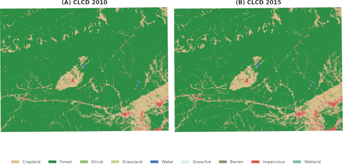
Figure 3. Observed land-use patterns in the Yixian–Huangshan landscape in 2010 and 2015. China Land Cover Dataset (CLCD) maps showing the spatial distribution of nine land-use classes within the analytical extent. (A) Observed land use in 2010. (B) Observed land use in 2015. Land-use classes comprise cropland, forest, shrub, grassland, water, snow/ice, barren land, impervious surfaces, and wetland. Please click here to view a larger version of this figure.
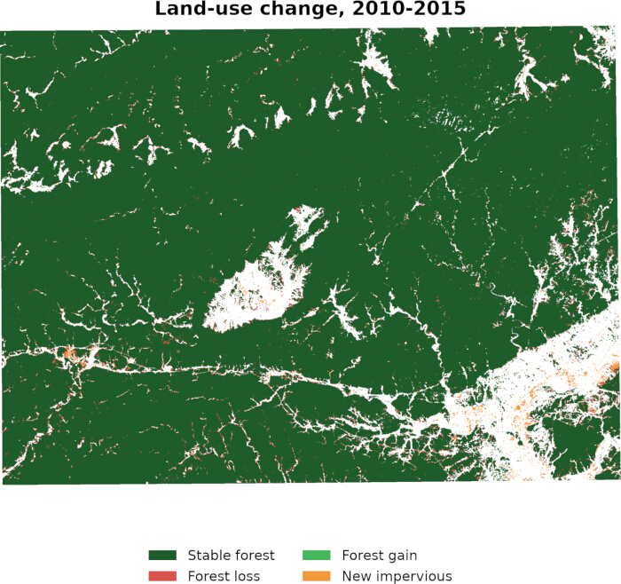
Figure 4. Observed land-use change in the Yixian–Huangshan landscape from 2010 to 2015. The map shows the spatial distribution of stable forest, forest loss, forest gain, and newly developed impervious surfaces between the 2010 and 2015 China Land Cover Dataset maps. White areas represent locations not classified into these four displayed change categories. Please click here to view a larger version of this figure.
Terrain characteristics and topographic heterogeneity
Within the valid mask, elevation ranged from 82.3 to 1,830.3 m (mean, 388.0 m), slope from 0 to 87.3° (mean, 22.4°), northness from −1 to 1, and topographic relief from 3.2 to 1,398.2 m (mean, 230.0 m). Relief was defined as the local elevation range within a circular neighborhood of 450 m radius, implemented with a 31 × 31-pixel footprint. Figure 5A–D shows elevation, slope, northness, and topographic relief, respectively. These layers characterize spatial terrain variation; any corresponding ecological mechanism is treated as a hypothesis rather than a causal result35,36,37,38,39,40,41,42,43,44.

Figure 5. Topographic variables used in the association analysis. Spatial distributions of the four topographic variables across the analytical extent: (A) elevation, expressed in meters; (B) slope, expressed in degrees; (C) northness, expressed on a scale from −1 to 1; and (D) topographic relief, expressed in meters. These variables were used in the optimal parameters-based geographical detector analysis of their individual and joint associations with 2015 carbon density. Please click here to view a larger version of this figure.
Multi-scenario land-use projections
The common transition matrix and scenario parameters summarized in Table 2 produced distinct aggregate trajectories using the numerical land-cover class identifiers provided in Supplementary Table 2. Figure 6 presents the observed and projected shares of forest, cropland, and impervious surfaces, whereas Figure 7A–D shows the BAU, TED, ECP, and VRA spatial projections for 2030, respectively, and Figure 7E–H shows the corresponding projections for 2050. By 2050, forest cover was projected to comprise 78.0% under BAU, 74.6% under TED, 80.3% under ECP, and 78.2% under VRA; the corresponding impervious shares were 6.3%, 17.6%, 2.8%, and 9.0%. Relative to observed 2015, projected impervious expansion was approximately 202 km2 under BAU, 675 km2 under TED, 57 km2 under ECP, and 317 km2 under VRA. These values are stress-test outputs rather than fitted forecasts. Projected changes are spatially clustered because candidate ranking uses target-class neighborhood counts and non-cropland conversion to impervious land is limited to edge cells. The model includes no transport-corridor, village-node, protected-area, ecological-redline, or statutory-planning layer; therefore, apparent alignment with specific infrastructure or regulated zones does not represent an encoded effect.
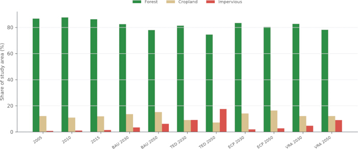
Figure 6. Observed and projected shares of major land-use classes under four scenarios. The percentage of the study area occupied by forest, cropland, and impervious surfaces is shown for the observed years 2005, 2010, and 2015 and for projections to 2030 and 2050 under the Business As Usual (BAU), Tourism Expansion and Development (TED), Ecological Conservation Priority (ECP), and Village Revitalization and Activation (VRA) scenarios. Bars represent the modeled share of the total study area for each land-use class; error bars are not applicable because the values are deterministic scenario outputs rather than replicate-based estimates. Please click here to view a larger version of this figure.
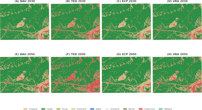
Figure 7. Projected spatial distribution of land use under four scenarios in 2030 and 2050. Projected land-use patterns under the Business As Usual (BAU), Tourism Expansion and Development (TED), Ecological Conservation Priority (ECP), and Village Revitalization and Activation (VRA) scenarios. (A–D) BAU, TED, ECP, and VRA projections, respectively, for 2030. (E–H) BAU, TED, ECP, and VRA projections, respectively, for 2050. Land-use classes comprise cropland, forest, shrub, grassland, water, snow/ice, barren land, impervious surfaces, and wetland. All scenario simulations were initialized from the observed 2015 CLCD map; therefore, cells with no simulated land-use transition retain their 2015 land-use class and baseline spatial pattern. Please click here to view a larger version of this figure.
Carbon storage dynamics under multi-scenario projections
Application of the complete four-pool lookup in Table 3 yielded 59.505 Tg C for 2015, equivalent to a mean density of 142.73 Mg C ha−1. Forest accounted for 57.04 Tg C (95.9%), whereas cropland accounted for 2.37 Tg C (4.0%). Impervious land made a small but nonzero contribution because the adopted source assigns this class 9.28 Mg C ha−1. Within the forest class, soil, aboveground, belowground, and dead-organic pools represented 53.5%, 33.8%, 10.9%, and 1.8% of total carbon, respectively31,32,33,34,44,47. All scenarios yielded lower carbon storage in 2050 than in 2015. Projected storage was 54.895 Tg C under BAU (a 7.75% loss), 51.475 Tg C under TED (13.49%), 56.523 Tg C under ECP (5.01%), and 54.540 Tg C under VRA (8.34%). The ECP–TED difference was 5.048 Tg C. These contrasts result from the imposed numerical parameters and do not estimate the effects of named policies. Figure 8A presents total carbon storage in 2015 and the scenario projections for 2030 and 2050; Figure 8B presents the corresponding mean carbon densities; Figure 8C presents carbon loss by 2050 relative to the 2015 baseline; and Figure 8D shows the relationship between projected forest share and carbon loss. The values are deterministic scenario outputs rather than replicate-based estimates.
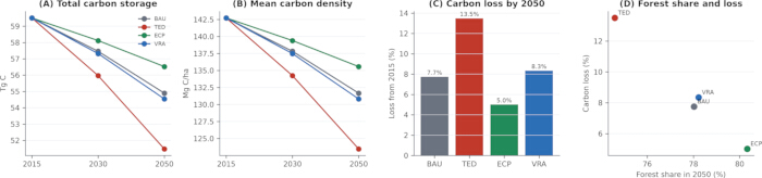
Figure 8. Projected carbon storage and its relationship with forest cover under four land-use scenarios. (A) Total carbon storage in 2015 and projected for 2030 and 2050 under the Business As Usual (BAU), Tourism Expansion and Development (TED), Ecological Conservation Priority (ECP), and Village Revitalization and Activation (VRA) scenarios, expressed in teragrams of carbon (Tg C). (B) Mean carbon density for the corresponding years and scenarios, expressed in megagrams of carbon per hectare (Mg C ha-1). (C) Percentage loss in total carbon storage by 2050 relative to the 2015 baseline for each scenario. (D) Relationship between projected forest share of the study area in 2050 and percentage carbon loss relative to 2015 for each scenario. Values are deterministic scenario outputs; error bars are not applicable. Please click here to view a larger version of this figure.
Topographic associations with the spatial heterogeneity of carbon storage
The OPGD factor detector ranked slope first (q = 0.557), followed by topographic relief (q = 0.460), elevation (q = 0.352), and northness (q = 0.003), as shown in Figure 9A. With 999 permutations, the permutation p-value for each factor was 0.001, the minimum attainable value; analytic F-test p-values were also below 0.001. The complete factor- and interaction-detector statistics, including optimized discretization intervals and analytic and permutation p-values, are provided in Supplementary Table 3. Statistical significance is distinguished from effect size: the association with northness was negligible in practical terms, and all q-values represent associations within the four assessed terrain variables rather than causal effects10,40. All factor pairs yielded interaction q-values greater than the larger of their individual q-values. The strongest interactions were slope ∩ relief (q = 0.628), elevation ∩ slope (q = 0.618), and elevation ∩ relief (q = 0.510), as shown in Figure 9B. These values indicate stronger stratified associations for paired factors but do not establish a geomorphological mechanism because soil, climate, forest age, management, and accessibility were not modeled.
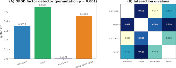
Figure 9. Topographic associations with 2015 carbon density identified using the optimal parameters-based geographical detector. (A) Factor-detector q-statistics for elevation, slope, northness, and topographic relief. The respective q-values are 0.3518, 0.5571, 0.0031, and 0.4600; permutation tests yielded p = 0.001. (B) Interaction-detector q-values for pairwise combinations of the four topographic variables. Larger q-values indicate stronger statistical associations with the spatial distribution of 2015 carbon density. OPGD, optimal parameters-based geographical detector. Please click here to view a larger version of this figure.
Overall outcomes
Figure 10A–D summarizes the principal outcomes of the workflow: projected forest share, total carbon storage, the ranking of topographic associations, and the key quantitative indicators, respectively. The 2015 analytical baseline contained 59.505 Tg C. Across the four exploratory parameter sets, projected losses by 2050 ranged from 5.01% to 13.49%, and all matched sensitivity cases preserved the ranking ECP > BAU > VRA > TED. Slope and relief showed the strongest assessed terrain associations. Given FoM = 0.107 and the omission of explicit planning, socioeconomic, and climate layers, the results support comparative regional assessment rather than deterministic spatial prediction.
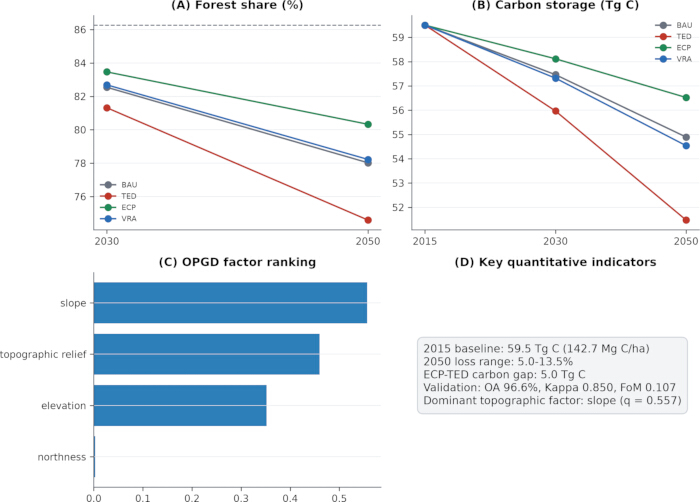
Figure 10. Summary of projected land-use and carbon-storage outcomes and topographic associations. (A) Projected forest share of the study area in 2030 and 2050 under the Business As Usual (BAU), Tourism Expansion and Development (TED), Ecological Conservation Priority (ECP), and Village Revitalization and Activation (VRA) scenarios; the dashed line indicates the 2015 baseline forest share. (B) Total carbon storage in 2015 and projected for 2030 and 2050 under the four scenarios, expressed in teragrams of carbon (Tg C). (C) Ranking of elevation, slope, northness, and topographic relief according to the q-statistics obtained using the optimal parameters-based geographical detector (OPGD), with larger q-values indicating stronger statistical associations with 2015 carbon density. (D) Summary of key quantitative indicators, including baseline carbon storage and density, projected 2050 carbon-loss range, difference in carbon storage between the ECP and TED scenarios, validation metrics, and the strongest assessed topographic association. OA, overall accuracy; FoM, Figure of Merit; Mg C ha-1, megagrams of carbon per hectare. Please click here to view a larger version of this figure.
Supplementary Figure 1. One-at-a-time sensitivity analysis of 2050 carbon storage under the four land-use scenarios. (A) Nominal 2050 carbon storage and the full OAT sensitivity range for BAU, TED, ECP, and VRA. Points indicate nominal scenario values, and vertical ranges indicate the minimum and maximum carbon-storage values obtained by multiplying one of dev, fp, or af by 0.5 or 1.5 while holding the other parameters constant. (B) Change in 2050 carbon storage relative to the corresponding nominal scenario value following 0.5× and 1.5× perturbations of dev, fp, and af. Values above zero indicate greater carbon storage than the nominal case, and values below zero indicate lower carbon storage. The ranges represent deterministic one-at-a-time parameter perturbations and are not probabilistic confidence intervals.Please click here to download this file.
Supplementary Table 1. Land-use transition matrix, scenario parameterization, model validation, and one-at-a-time sensitivity-analysis results. The workbook contains four worksheets: S1, the 2010–2015 operational land-use transition matrix; S2, parameter values, implemented rules, and interpretation boundaries for the four scenarios; S3, the 9 × 9 confusion matrix and associated model-validation results; and S4, nominal and one-at-a-time sensitivity results obtained by varying dev, fp, and af by 0.5× and 1.5× while holding the other parameters constant. Sensitivity ranges represent deterministic parameter perturbations and are not probabilistic confidence intervals.Please click here to download this file.
Supplementary Table 2. Land-cover class identifiers used in the computational workflow. The table lists the numerical class identifiers and corresponding land-cover classes used in the raster analyses. Class 0 denotes NoData outside the valid study-area mask; classes 1–9 denote cropland, forest, shrub, grassland, water, snow/ice, barren, impervious, and wetland, respectively.Please click here to download this file.
Supplementary Table 3. OPGD factor- and interaction-detector results for 2015 carbon density. The table reports optimized q-statistics, numbers of discretization intervals, analytic F-test p-values, and permutation p-values based on 999 permutations for elevation, slope, northness, and topographic relief. Pairwise interaction results report the interaction q-statistic, individual factor q-statistics, and interaction classification. The reported statistics represent spatial associations and do not establish causal effects.Please click here to download this file.
Supplementary Note 1. Panel-by-panel descriptions, data sources, and interpretation notes for the manuscript figures. The note identifies the content and underlying data source for individual figure panels and provides information concerning shared spatial extents, duplicated information, and interpretation of the displayed variables.Please click here to download this file.
Supplementary Data Archive (zipped). The archive contains 26 analysis-ready GeoTIFF files, boundary files, metadata, results, scripts, figures, workbooks, exact computational environment files, a README file, and SHA-256 checksums.
Discussion
Across the four stress tests, carbon storage declined as simulated transitions altered the proportions of high- and lower-density land-cover classes. TED produced the greatest decline, whereas ECP produced the smallest. A critical step in applying the protocol is therefore the configuration and interpretation of the dev, fp, and af parameters. Because the scenario differences arise from these imposed values, they represent conditional model responses rather than observed effects of tourism development, village revitalization, or ecological regulation. By 2050, projected carbon storage under TED was 5.048 Tg C lower than under ECP. Under the adopted lookup, converting one hectare of forest to impervious land reduces the assigned stock by 149.32 Mg C, whereas conversion from cropland to impervious land reduces it by 38.45 Mg C. These accounting contrasts explain the strong influence of simulated forest conversion on total storage. However, reliance on literature-derived values without local calibration introduces uncertainty into the absolute estimates.
Another critical step is the derivation and discretization of the terrain variables used in OPGD. Topographic relief was associated with carbon density after optimized discretization (q = 0.460). Relief was defined as the local elevation range within a circular neighborhood of 450 m radius, implemented with a 31 × 31-pixel footprint. High-relief cells may coincide with steep, forested terrain, but OPGD cannot distinguish among terrain, accessibility, land-use history, soil, management, and other correlated explanations. Paired terrain strata produced stronger q-values than individual factors, particularly for slope ∩ relief (q = 0.628). This pattern is descriptive rather than mechanistic. Similarly, the small q-value for northness (0.003) does not demonstrate that contrasts in solar radiation are weak; testing this explanation requires radiation, microclimate, vegetation, and field measurements.
The method supports regional hypothesis generation: limiting simulated forest conversion, moderating impervious expansion, and increasing cropland-to-forest transition preserve more assigned carbon. Site-specific prescriptions require additional evidence. For modification of the workflow toward decision-focused applications, incorporate verified protected-area, ecological-redline, transport, parcel, and village-node layers, together with assessments of stakeholder participation, ecosystem-service trade-offs, incentives, restoration costs, cultural services, livelihoods, and biodiversity49,50,51,52,53,54,55,56. These extensions are important because the current protocol does not encode such spatial or socioeconomic constraints. The broader literature also indicates that plant storage strategies, forest structure, non-tree vegetation, tourism behavior, and built-environment life-cycle effects require analyses distinct from the present land-cover accounting57,58,59,60,61.
Several limitations define the appropriate use and interpretation of the method. These include literature-derived carbon densities without local field calibration, potential CLCD classification error, a simplified custom Markov-CA, a change-focused validation FoM of 0.107, non-fitted stress-test parameters, and a single-seed stochastic assessment. Additional limitations are the one-factor-at-a-time design rather than probabilistic uncertainty analysis, omission of planning, socioeconomic, accessibility, soil, forest-age, and climate-change layers, and non-causal OPGD associations. These limitations mean that the workflow is appropriate for comparative regional scenario assessment but does not provide deterministic spatial forecasts, locally calibrated carbon inventories, or causal estimates of policy effectiveness.
With respect to existing and alternative approaches, the significance of the protocol lies in integrating land-use simulation, four-pool carbon accounting, validation, sensitivity testing, and terrain-association analysis within a reproducible workflow while retaining explicit limitations on interpretation. Troubleshooting and modification should focus particularly on the steps that most strongly affect downstream interpretation: land-cover preprocessing and masking, transition and scenario parameterization, model validation, carbon-density assignment, and terrain discretization.
The workflow can be applied to comparative assessment of alternative land-use trajectories and to identifying spatial associations that warrant further investigation, while site-specific applications require additional locally verified evidence. Priorities for future research include collecting local carbon measurements, comparing alternative allocation models and random seeds, fitting parameters to independent drivers, and propagating classification, parameter, and climate uncertainty. These developments would extend the present workflow beyond comparative stress testing and provide a stronger basis for evaluating land-use and carbon-storage outcomes under additional sources of uncertainty.
Disclosures
The authors declare no conflicts of interest.
Acknowledgements
The authors thank the providers of the CLCD and Copernicus DEM GLO-30 datasets.
Materials
| Name | Company | Catalog Number | Comments |
|---|---|---|---|
| China Land Cover Dataset (CLCD) | Wuhan University (Yang J & Huang X) | 1985–2022 annual product; 30 m; Zenodo DOI: 10.5281/zenodo.4417810 | Base land-cover input; 2005, 2010, and 2015 layers used for calibration, validation, transition-matrix estimation, and baseline analysis |
| Copernicus DEM GLO-30 | European Space Agency / Copernicus Programme | Reference epoch 2019; 2021 public release; 30 m | Terrain input used to derive elevation, slope, northness, and topographic relief for OPGD analysis |
| Custom Markov cellular automaton | Custom Python implementation | Python 3.11; seed 2023; synchronous update; 3 × 3 Moore neighborhood; archived source | Land-use scenario simulation; custom implementation that does not invoke PLUS |
| geopandas (Python library) | geopandas developers | 1.1.4 | Vector-data handling, spatial queries, and boundary operations |
| InVEST four-pool carbon-storage formulation | Natural Capital Project | InVEST documentation; custom Python lookup calculation; archived script | Class-based four-pool carbon accounting; no sequestration-rate, valuation, or economic module |
| matplotlib (Python library) | Matplotlib developers | 3.11.0 | Figure rendering and scientific visualization |
| numpy (Python library) | NumPy developers | 2.4.6 | Array-level numerical computation |
| OPGD factor and interaction detectors | Custom Python implementation based on OPGD methodology | Seed 42; 200,000-pixel sample; 2–15 quantile intervals; 999 permutations; archived script | Factor and interaction analysis of associations between 2015 carbon density and elevation, slope, northness, and topographic relief |
| pandas (Python library) | pandas developers | 3.0.3 | Tabular-data handling and analytical output processing |
| Python programming language | Python Software Foundation | 3.11.9 | Computational environment for preprocessing, simulation, validation, carbon accounting, OPGD analysis, and postprocessing |
| rasterio (Python library) | rasterio maintainers | 1.4.4 | Raster input/output, reprojection, resampling, and processing of land-cover and terrain rasters |
| scipy (Python library) | SciPy developers | 1.17.1 | Numerical and morphological operations used in terrain processing |
| shapely (Python library) | Shapely developers | 2.1.2 | Geometric operations supporting vector and spatial processing |
| Study-area extent and valid mask | Custom study input reconstructed from manuscript coordinates | EPSG:32650; 30 m; archived GeoJSON and GeoTIFF; 4,632,329 valid cells | Defines the 4,169.1 km² common analysis area and valid raster mask |
References
- Costanza R, et al. The value of the world's ecosystem services and natural capital. Nature. 1997;387(6630):253-260. doi:10.1038/387253a0.
- Millennium Ecosystem Assessment. Ecosystems and Human Well-Being: Synthesis. Island Press; Washington, DC; 2005.
- UNESCO World Heritage Centre. Mount Huangshan [Internet]. UNESCO; Paris; [cited 2026 Aug 18]. Available from: https://whc.unesco.org/en/list/547
- UNESCO World Heritage Centre. Ancient Villages in Southern Anhui—Xidi and Hongcun [Internet]. UNESCO; Paris; [cited 2026 Aug 18]. Available from: https://whc.unesco.org/en/list/1002
- Megarry WP, et al. Land use and land cover analysis of cultural World Heritage to inform assessments of climate vulnerability. Journal of Cultural Heritage. 2026;77:243-253. doi:10.1016/j.culher.2025.11.008.
- Wang Y, Chen S, Rabeeu A. Does world heritage site initiation promote tourism? A difference-in-difference approach. Tourism Economics. 2024;30(8):2111-2133. doi:10.1177/13548166241253306.
- Wang Y, Sulaiman MKAM, Harun NZ. Reframing place identity for traditional village conservation: A theoretical model with evidence from Dali Dong Village. Heritage. 2025;8(10):427. doi:10.3390/heritage8100427.
- Liang X, et al. Understanding the drivers of sustainable land expansion using a patch-generating land use simulation (PLUS) model: A case study in Wuhan, China. Comput Environ Urban Syst. 2021;85:101569. doi:10.1016/j.compenvurbsys.2020.101569.
- Sharp R, et al. InVEST User's Guide: Integrated Valuation of Ecosystem Services and Tradeoffs. [Internet]. Natural Capital Project, Stanford University; 2020. Available from: https://naturalcapitalproject.stanford.edu/software/invest
- Song Y, Wang J, Ge Y, Xu C. An optimal parameters-based geographical detector model enhances geographic characteristics of explanatory variables for spatial heterogeneity analysis: cases with different types of spatial data. GISci Remote Sens. 2020;57(5):593-610. doi:10.1080/15481603.2020.1760434.
- Bozali N. Spatiotemporal simulation of land use and land cover changes in Türkiye through a CA–Markov framework. Scientific Reports. 2026;16(1). doi:10.1038/s41598-026-35807-9.
- Gita B, Pankaj L. Modeling alternative futures: Scenario-based land-use and land-cover projections for Nepal (2030–2050). Land. 2026;15(5):873. doi:10.3390/land15050873.
- Cui J, et al. An integrated land use–carbon modeling framework for net carbon emissions and spatial optimization in Northeast China. Journal of Cleaner Production. 2025;525:146545. doi:10.1016/j.jclepro.2025.146545.
- Tang H, et al. Analysis of spatiotemporal variations and driving factors of carbon storage based on the PLUS-InVEST-OPGD model: A case study of Tai'an City. Sustainability. 2026;18(8):4017. doi:10.3390/su18084017.
- Zhang Y, Liao X, Sun D. A coupled InVEST-PLUS model for the spatiotemporal evolution of ecosystem carbon storage and multi-scenario prediction analysis. Land. 2024;13(4):509. doi:10.3390/land13040509.
- Huang M, et al. Integrated assessment of land use and carbon storage changes in the Tulufan-Hami Basin under the background of urbanization and climate change. Int J Appl Earth Obs Geoinf. 2024;135:104261. doi:10.1016/j.jag.2024.104261.
- Ma Y, et al. Assessing carbon storage dynamics and policy impacts: Application of InVEST-PLUS framework in the Qinling Mountains, China. Land Use Policy. 2026;164:107947. doi:10.1016/j.landusepol.2026.107947.
- Li Z, Yan T, Du Y. Scenario-based simulation of carbon storage in Chengdu using MCCA-InVEST: land use change, spatial patterns, and driving mechanisms. Carbon Balance Manag. 2025;20:40. doi:10.1186/s13021-025-00328-x.
- Zhao H, Guo B, Wang G. Spatial-temporal changes and prediction of carbon storage in the Tibetan Plateau based on PLUS-InVEST model. Forests. 2023;14(7):1352. doi:10.3390/f14071352.
- Hasan F, Makhtoumi Y, Chen G. Impact of land use and land cover changes on ecosystem services: a multi-module InVEST-LCM analysis. Earth Syst Environ. 2026;10:7019-7041. doi:10.1007/s41748-025-00995-3.
- Zhang H, Luo J, Wu J, Dong H. Dynamic response of carbon storage to future land use/land cover changes motivated by policy effects and core driving factors. J Plant Ecol. 2024;17(4):rtae042. doi:10.1093/jpe/rtae042.
- Lu L, et al. Spatiotemporal variation and quantitative attribution of carbon storage based on multiple satellite data and a coupled model for Jinan City, China. Remote Sens. 2023;15(18):4472. doi:10.3390/rs15184472.
- Ma J, Hao Z, Shen Y, Zhen Z. Spatial-temporal evolution of carbon storage and its driving factors in the Shanxi section of the Yellow River Basin, China. Ecological Modelling. 2025;502:111039. doi:10.1016/j.ecolmodel.2025.111039.
- Mi Y, Li S, Wu B. Study on the variation of carbon storage in the Chang-Zhu-Tan urban agglomeration in China based on topographic relief. Frontiers in Environmental Science. 2024;12. doi:10.3389/fenvs.2024.1481540.
- Li C, Huang J, Luo Y, Wang J. Spatial synergy between carbon storage and emissions in coastal China: Insights from PLUS-InVEST and OPGD models. Remote Sensing. 2025;17(16):2859. doi:10.3390/rs17162859.
- Ocloo DM, Mizunoya T. Carbon storage and land use dynamics in Ghanaian university campuses: A scenario-based assessment using the InVEST model. Land. 2025;14(10):1987. doi:10.3390/land14101987.
- Wang Z, Zhang Y, Zhang Z. Scenario analysis of carbon reduction potential through forest carbon sink mechanisms in the Beijing–Tianjin–Hebei Region, China. Sustainability. 2025;17(17):7992. doi:10.3390/su17177992.
- Ma J, Shi P. Remotely sensed inter-field variation in soil organic carbon content as influenced by the cumulative effect of conservation tillage in northeast China. Soil and Tillage Research. 2024;243:106170. doi:10.1016/j.still.2024.106170.
- Li M, Cui Y, Dong J, Qin Y. Abandoned cropland compensates the decrease in net ecosystem productivity of impervious surface expansion in China. Environmental Impact Assessment Review. 2024;104:107363. doi:10.1016/j.eiar.2023.107363.
- Wang J, Zhang M, Zhou S, Huang Y. Research on the spatiotemporal evolution and driving factors of forest carbon sink increment—based on data envelopment analysis and production theoretical decomposition model. Forests. 2025;16(1):104. doi:10.3390/f16010104.
- Cai Y, et al. Dynamics of China's forest carbon storage: the first 30 m annual aboveground biomass mapping from 1985 to 2023. Earth System Science Data. 2025. doi:10.5194/essd-17-6993-2025.
- Piao S, et al. The carbon balance of terrestrial ecosystems in China. Nature. 2009;458(7241):1009-1013. doi:10.1038/nature07944.
- Fuller M, et al. Global carbon storage in harvested wood products: a forest sector model inter-comparison. Environmental Research Letters. 2025;20. doi:10.1088/1748-9326/ae0ce0.
- Milodowski D, Smallman T, Williams M. Scale variance in the carbon dynamics of fragmented, mixed-use landscapes estimated using model–data fusion. Biogeosciences. 2023. doi:10.5194/bg-20-3301-2023.
- Zeyu X, et al. Topographic and edaphic drivers of community structure and species diversity in a subtropical deciduous broad-leaved forest in eastern China. Forests. 2025;16(12):1837. doi:10.3390/f16121837.
- Hunter BD, Roering JJ, Silva LCR, Moreland KC. Geomorphic controls on the abundance and persistence of soil organic carbon pools in erosional landscapes. Nature Geoscience. 2024;17(2):151-157. doi:10.1038/s41561-023-01365-2.
- Li L, et al. Spatial scale effects of interacting abiotic and biotic factors on aboveground carbon storage in a subtropical evergreen broadleaf forest in southern China. Journal of Forestry Research. 2024;36(1). doi:10.1007/s11676-024-01804-9.
- Zhaoxue G, et al. Temporal and spatial characteristics and influencing factors of carbon storage in black soil area under topographic gradient. Land. 2024;14(1):16. doi:10.3390/land14010016.
- Nie Q, et al. Exploring scaling differences and spatial heterogeneity in drivers of carbon storage changes: a comprehensive geographic analysis framework. Ecological Indicators. 2024. doi:10.1016/j.ecolind.2024.112193.
- Liu J, et al. Analysis of the evolution characteristics and driving mechanisms of salinization in arid regions based on multi-factor interaction with optimized parameter geographic detector (OPGD)1. Journal of Environmental Management. 2025;394:127487. doi:10.1016/j.jenvman.2025.127487.
- Wang Z, Zhou Y, Sun X, Xu Y. Estimation of NPP in Huangshan District based on deep learning and CASA model. Forests. 2024;15(8):1467. doi:10.3390/f15081467.
- Vancine MH, et al. ATLANTIC SPATIAL: a dataset of landscape, topographic, hydrological, and anthropogenic metrics for the Atlantic Forest. Ecology. 2026;107(4). doi:10.1002/ecy.70360.
- Qiu M, et al. Spatio-temporal changes and hydrological forces of wetland landscape pattern in the Yellow River Delta during 1986–2022. Landscape Ecology. 2024;39. doi:10.1007/s10980-024-01850-y.
- Anand S, Khushboo K, Garkoti S. Influence of vegetation and soil properties on carbon stocks in Shorea robusta. forests under different disturbance regimes. Journal of Environmental Management. 2025;380:124916. doi:10.1016/j.jenvman.2025.124916.
- Yang J, Huang X. The 30 m annual land cover dataset and its dynamics in China from 1990 to 2019. Earth Syst Sci Data. 2021;13(8):3907-3925. doi:10.5194/essd-13-3907-2021.
- Copernicus Data Space Ecosystem. Copernicus DEM GLO-30 [Internet]. European Union; [cited 2026 Aug 18]. Available from: https://documentation.dataspace.copernicus.eu/Data/Others/CCM.html
- Cheng Z, et al. Identification of eco-functional zones based on ecosystem service bundles: a case study of the Fujiang River Basin. Front Environ Sci. 2026;14:1754712. doi:10.3389/fenvs.2026.1754712.
- Pontius RG Jr, et al. Comparing the input, output, and validation maps for several models of land change. Ann Reg Sci. 2008;42(1):11-37. doi:10.1007/s00168-007-0138-2.
- Li Y, et al. Dissemination, manipulation or monopolization? Understanding the influence of stakeholder information sharing on resident participation in neighborhood rehabilitation of urban China. Land Use Policy. 2024;147:107359. doi:10.1016/j.landusepol.2024.107359.
- Peng J, et al. A landscape ecological approach to spatial conservation planning—ecological security pattern. Trends in Ecology & Evolution. 2025. doi:10.1016/j.tree.2025.07.014.
- Roh H, Park J, Chon J. Trade-off analysis of ecosystem services in regulated river areas: supporting, regulating, and cultural services. Sustainability. 2025;17(9):3788. doi:10.3390/su17093788.
- Roy Chowdhury PK, Brown DG. Modeling the effects of carbon payments and forest owner cooperatives on carbon storage and revenue in Pacific Northwest forestlands. Land Use Policy. 2023;131:106725. doi:10.1016/j.landusepol.2023.106725.
- Savo V, et al. Evaluation of main regulating, provisioning, and supporting ecosystem services of urban street trees: a literature review. Ecosystem Services. 2025;71:101690. doi:10.1016/j.ecoser.2024.101690.
- Shibo Z, Gui J. The cost of ecological protection and restoration: evidence from the impact of the Shan-shui project on land values. Land Use Policy. 2026;164:107919. doi:10.1016/j.landusepol.2026.107919.
- Deng H, Zhou X, Liao Z. Ecological redline delineation based on the supply and demand of ecosystem services. Land Use Policy. 2024;140:107109. doi:10.1016/j.landusepol.2024.107109.
- Xu H, et al. Revealing youth-perceived cultural ecosystem services for high-density urban green space management: a deep learning spatial analysis of social media photographs from central Beijing. Landscape Ecology. 2025;40. doi:10.1007/s10980-025-02115-y.
- Binter J, Doležal J. High-elevation angiosperms maintain extensive living storage tissue with large non-structural carbohydrate pools. Annals of Botany. 2026. doi:10.1093/aob/mcag023.
- Arayaselassie A, Bekele T, Lulekal E. An insight into Northern Wollo Monastery Forests: examining plant species diversity, vegetation structure, and regeneration analysis of these relict ecosystems. PLoS ONE. 2025;20. doi:10.1371/journal.pone.0330689.
- Slate ML, et al. Impact of changing climate on bryophyte contributions to terrestrial water, carbon, and nitrogen cycles. New Phytologist. 2024;242. doi:10.1111/nph.19772.
- Sun D, Yang D, Wang J, Tan F. How animal metaphors increase tourists' waste classification intention? Environmental Research Communications. 2024;6(10):105012. doi:10.1088/2515-7620/ad82b0.
- Sindhu Pradeep M, Rismanchi B, Stephan A, Ngo T. Synergising circularity and temporal dynamics into life cycle sustainability assessment of prefabricated buildings: a system dynamics-based assessment with static–dynamic comparison. Building and Environment. 2026;302:114795. doi:10.1016/j.buildenv.2026.114795.
Reprints and Permissions
This article has been published
Video Coming Soon