This research work presented an approach, FusionNetX, by enriching the feature fusion capability of DenseNet121 and EfficientNetB7 for the classification of brain tumors on five publicly available datasets with data augmentation, preprocessing, and hybrid model customization (intermediate Fusion), achieving results ranging from 98.77% to 99.89%, outperforming across multiple evaluation parameters.
A subscription to JoVE is required to view this content. Sign in or start your free trial.
Method Article
FusionNetX: A Deep Feature Fusion Model Leveraging MRI and Deep Learning for Enhanced Brain Tumor Detection
In This Article
Summary
Abstract
Brain tumors are considered one of the deadliest diseases in the world, and misdiagnosing them puts patients’ lives in danger and lowers the survival rate. Magnetic resonance imaging (MRI) with deep learning-based techniques, especially convolutional neural networks, is crucial for overcoming this obstacle, as it enables a more detailed examination of the brain's internal structure and offers outstanding learning and predictive capabilities. The need for accurate diagnosis of the tumor in the brain is still significant. Therefore, an enhanced feature-fusion-based DL model (FusionNetX) is proposed that leverages the strengths of two pretrained models, DenseNet121 and EfficientNetB7, using customized fine-tuning hyperparameters, including trainable and non-trainable layers. The proposed FusionNetX model was applied to five publicly available brain tumor datasets: Br35H, Figshare, Sartaj, Masoud, and Balanced Brain Tumor. Some preprocessing steps were applied to improve image quality and address overfitting through resizing and data augmentation. Using a variety of performance evaluation metrics, such as accuracy, loss, positive predicted value, negative predictive value, true positive rate, true negative rate, F1-score, false negative rate, and false positive rate, the proposed model FusionNetX was found to have an accuracy of 99.33% for Br35H, 99.13% for Figshare, 99.89% for Masoud, 99.19% for BBT-Dataset, and 98.77% for Sartaj. Additionally, the five brain tumor datasets were evaluated using late fusion and attention-based fusion to demonstrate the significance of the proposed FusionNetX model, and the results were substantially better, with gains of 0.3% to 1.9% across all datasets. Furthermore, the receiver operating characteristic curve is computed, and results from various performance evaluation metrics indicate that the proposed FusionNetX model can accurately detect and predict brain tumors and help health practitioners make timely decisions.
Introduction
Cancer is the deadliest disease in the human body nowadays because of its severity and growing rate, while multiple cancerous diseases, like brain tumors, breast cancer, lung nodules, kidney cancer, and others, are found in the human body, causing an increase in the death rate. Cancer develops when cells or tissues in a person's body multiply abnormally. When cancer metastasizes, it can damage other human organs and become more dangerous1. Because the brain controls every bodily function, any damage to it can have far-reaching consequences for the entire body. That is why brain tumors or cancer are so lethal to humans2. Additionally, benign and malignant brain tumors are the two main categories into which they fall. "Benign" basically means not cancerous; it's merely a problem in the brain that can be fixed by changing the surroundings. But in the case of malignancy, it is considered dangerous because of its metastatic nature, for moving abnormal cells or tissues to move to or from other body parts, disturbing other organs as well, by increasing the cancer's chance in the body3.
Also, according to the American Brain Tumor Association and the World Health Organization (WHO), pituitary tumors, meningiomas, and gliomas are the three main categories of brain cancers4. Gliomas originate from glial cells, which nourish neurons in the brain. Pituitary tumors begin in the pituitary gland, situated at the base of the brain and responsible for various bodily functions; meningioma tumors, on the other hand, begin in the meninges, which safeguard the membranes encircling the brain and spinal cord. Furthermore, multiple medical imaging modalities are commonly used to examine the internal parts of the body for diagnostic purposes, including X-rays, computed tomography (CT) scans, and magnetic resonance imaging (MRI)5,6. Each imaging modality has its own pros and cons. MRI is an imaging modality that provides detailed images of soft tissues and cells in the body, especially in the brain. Cancer involves abnormal tissue or cells in the body, and MRI provides detailed images of these abnormalities, making it a more useful imaging modality for diagnosing brain tumors or cancer. Additionally, MRI is safer than other imaging modalities because it does not produce harmful radiation during examinations of internal body anatomy.
Additionally, many computational methodologies are also employed to address the diagnostic challenges associated with brain tumors, including machine learning (ML), image processing (IP), and deep learning (DL), and each approach is applied to images taken by imaging modalities to diagnose the cancer7. These approaches learn the hidden patterns and structures of different objects in images to diagnose cancer by identifying patterns in the affected region. Each computational approach has its own pros and cons in the diagnosis process. ML and IP-based approaches extract handcrafted features, which mostly lead to inaccurate predictions and misdiagnose the process, especially on larger datasets8. To overcome issues with handcrafted feature extraction, people are moving toward deep learning-based models, commonly called convolutional neural network (CNN)-based models, that learn and automatically extract the best features from images to accurately diagnose tumors. DL-based approaches are now commonly used in medical imaging to diagnose diseases in the human body, especially for early and accurate detection of brain tumors, breast cancer, lung cancer, and other diseases, because of their ability to learn and extract complex patterns in large-scale data by producing more accurate results9. The main problem faced in a DL model is the consumption of more resources and data sampling, which is overcome by another deep learning-based approach called transfer learning10 (TL), In which pretrained models are used to diagnose the disease, saving time and resources. Early and accurate diagnosis of health issues is made possible by pretrained models, which have already learned basic features related to texture, color, edges, and more from a large dataset. These models can then be transferred to a new dataset that has never been seen before by leveraging the model and adding hyperparameters and trainable and non-trainable layers11. A significant amount of research has been conducted on the classification of brain tumors, and Table 112,13,14,15,16,17,18,19,20,21,22,23 presents the details of this research, including the approaches, datasets, and results. Still, no research work has employed a methodology that combines two transfer learning models for robust feature extraction and adjusts regularization techniques to ensure smooth training and testing. Excess evaluation of the proposed methodology provides insights into model performance across different brain tumor features.
| Ref | Approach | Data Samples | Results | Limitations |
| 12 | Customized CNN | Br35H | Accuracy = 97.45%, | There is still a need for improvements in the results; instead of using a self-made CNN, it’s better to use a pre-existing CNN model with modification. |
| Loss = 0.1141%, | ||||
| Recall = 98.09%, | ||||
| F1-Score = 97.69%, | ||||
| Precision = 97.29%, | ||||
| Augmented Br35H | Accuracy = 98.99%, | |||
| Precision = 98.90%, | ||||
| Loss = 0.0570%, | ||||
| Recall = 98.91%, | ||||
| F1-Score = 99.04% | ||||
| 13 | Feature Fusion DNN model | Br35H | Accuracy = 98.22%, | There is still a need for improvements in the results, and instead of using a customized model, there is still a still a need to use a preexisting model for feature fusion. |
| FNR = 1.77%, | ||||
| Sensitivity = 98.2%, | ||||
| F1-Score = 98%, | ||||
| Specificity = 98%, | ||||
| Figshare | Accuracy = 98.01%, | |||
| Sensitivity = 96.03%, | ||||
| F1-Score = 96%, | ||||
| Specificity = 98.67%, | ||||
| FNR = 3.96% | ||||
| 14 | AlexNet with SGD | Br35H | Accuracy = 98.79%, | Still, there is a need for some improvements in the results, and we also need to check some advanced CNN-based models on different data samples. |
| MCR = 1.20%, | ||||
| Sensitivity = 98.98%, | ||||
| Specificity = 98.58%, | ||||
| F1-Score = 98.82% | ||||
| 15 | InceptionV3 | Figshare | Accuracy = 98.89%, | The authors used the Figshare dataset, which has three classes of tumors; instead of classifying them, they classify either tumor exit or not, and there is still a need for improvements in results as well as categorizing the tumor classes. |
| SensitivityB = 95.28%, | ||||
| SensitivityM = 94.47% | ||||
| 16 | Optimized ResNet50 | Figshare | Accuracy = 99.03%, | Other performance evaluation parameters needed to be calculated with some more improvements in results. |
| Recall = 99%, | ||||
| F1-Score = 99% | ||||
| 17 | Res-BRNet | Br35H | Accuracy = 98.22%, | There is still need for improvements in the results. |
| Sensitivity = 98.11%, | ||||
| Precision = 98.22%, | ||||
| Figshare | F1-Score = 98.41% | |||
| 18 | ResNet101 + DenseNet121 | Figshare | Accuracy = 99.18%, | There is a little bit of improvement in the results and a need to check more brain tumor-related data sets. |
| Recall = 99.11%, | ||||
| F1-Score = 99.08, | ||||
| Precision = 99.07%, | ||||
| Sartaj | Accuracy = 97.24%, | |||
| Recall = 97.58%, | ||||
| F1-Score = 97.28%, | ||||
| Precision = 97.06%, | ||||
| 19 | CNN-SVM | Brats | Accuracy = 98.02%, | There is a need to apply some preexisting models with SVM, and there is still a need for improvements in the results. |
| F1-Score = 98.31%, | ||||
| Precision = 98.09%, | ||||
| Sensitivity = 98.53%, | ||||
| Specificity = 97.30%, | ||||
| Sartaj | Accuracy = 96.83%, | |||
| Precision = 95.36%, | ||||
| Sensitivity = 94.73%, | ||||
| Specificity = 97.56%, | ||||
| F1-Score = 95% | ||||
| 20 | Fine-tuned EfficientNetB3 | Figshare | Accuracy = 98.70% | There is a need for the aforementioned variants of EfficientNetB3 to improve the results. |
| Sartaj | Accuracy = 97.50% | |||
| 21 | InceptionV4 | Masoud | Accuracy = 98.7%, | Some improvements in the results required with using some more datasets. |
| Precision = 99%, | ||||
| Sensitivity = 98%, | ||||
| Specificity = 99%, | ||||
| F1-Score = 99.1% | ||||
| 22 | VGG16 | Masoud | Accuracy = 98% | There is a need for improvements in the results with checking more deep neural network models. |
| 23 | MFR-CNN | Masoud | Accuracy = 94%, | It’s a complex architecture used in this proposed solution. |
| Recall = 96%, | ||||
| F1-Score = 96%, | ||||
| Precision = 96%, |
Table 1: A comparative examination of the most recent research work. The table summarizes existing research, along with their approaches, data samples, results, and limitations. Please click here to download this Table.
Table 1 reviews existing approaches, highlighting their limitations in improving results and the necessity of using pre-existing DL models while evaluating their performance against various statistical parameters, all within an efficient framework that performs better on different brain tumor datasets.
Study objectives and problem statement
Manual interpretation is time-intensive and suffers from interobserver variability; thus, rapid and accurate categorization of brain tumor types from MRI is vital for clinical decision-making. Most DL approaches for automated brain tumor classification today are based on a single backbone network or simple decision-level fusion, which does not fully utilize the complementary feature representations from multiple pretrained architectures, and are often validated only on a single dataset, limiting confidence in their generalizability.
This research project aims to develop and provide a complete, accurate method for diagnosing brain cancers in human brains using a dual-backbone DL framework (EfficientNetB7 and DenseNet121) that leverages complementary feature representations to enable robust brain tumor classification from MRI. It also evaluates the framework's robustness across multiple independent public datasets. This approach can help radiologists and paramedics quickly and effectively diagnose brain tumors, saving patients' lives by enabling recognition and classification.
To solve a particular research problem and to achieve the aims or goals of this research project, the following are the research questions and the contribution to address those questions: 1) Is the feature-level (intermediate) fusing of two pretrained backbone networks better than the decision-level (late) and attention-based fusion techniques for brain tumor classification? 2) Will the suggested system provide consistent classification performance in many independently acquired brain tumor MRI datasets?
The scope of this study is restricted to image-level (2D MRI slice) classification, using five publicly available brain tumor MRI datasets (Br35H, Figshare, Sartaj, Masoud, and BBT-Dataset); evaluated independently, not inter-dataset; and using the specific architecture, preprocessing pipeline, and experimental configuration described in the methodology section. The study does not include patient-level validation or testing in a clinical deployment setting.
The major contributions of this research work are as follows: 1) The primary contribution of this research work is to utilize dual pretrained models for better feature extraction, including DenseNet121 and EfficientNetb7 with optimized hyperparameters. 2) Innovative model architecture with an advanced regularization technique integrated with concatenated features from a dual-pretrained model for robust performance. 3) An effective data augmentation strategy is applied to increase the diversity of the training samples to learn more generic and specific features, overcoming overfitting issues. 4) The proposed model's performance was assessed on five distinct publicly available brain tumor datasets, focusing on various statistical evaluation parameters, including accuracy, misclassification rate, precision, negative predictive value, sensitivity, specificity, F1-Score, false negative rate, and false positive rate.
Access restricted. Please log in or start a trial to view this content.
Protocol
The most threatening disease in the world is a brain tumor. An accurate diagnosis can be beneficial to patients’ survival. Still, there is a need for an accurate diagnostic system that can detect brain tumors at an early stage. To address this problem, a more reliable technique for accurately detecting brain tumors in their early stages has been proposed by using a hybrid dual deep learning mechanism with optimized hyperparameters and fine-tuned layers based on the DenseNet121 and EfficientNetB7 models. The proposed approach takes 2D MRI images as input and outputs a prediction of either tumor exit or no tumor exit for the binary classification dataset Br35H, and tumor categorization for four other multiclass classification datasets. So, this section demonstrates the major steps of the proposed approach, from data gathering to final output, including data acquisition, data preprocessing, data splitting, model selection, feature extraction, tumor prediction, and evaluation of the proposed model, as shown in Figure 1.
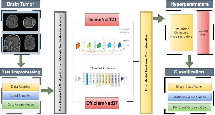
Figure 1: Proposed Methodology workflow. This diagram shows the overall architecture of the proposed model, including data acquisition and preprocessing; two pretrained models for feature extraction; concatenation of their features; and hyperparameter fine-tuning for tumor classification and type. Please click here to view a larger version of this figure.
Data acquisition
In any experimental research, the first step is data acquisition. For this, it has chosen five different publicly available datasets, including Br35H24, Figshare25, Sartaj26, Masoud27, and the brain tumor MRI image-based dataset from the open-source library Kaggle28, which have already been used by many research scholars for the diagnosis of brain tumor detection. The Br35H dataset has 3,000 images comprising two classes: healthy and unhealthy (tumor) brain images, with 1,500 in each class, while the Figshare dataset comprises 3,064 images, split into three groups based on tumor type. 1,426 images of glioma, 708 images of meningioma, and 930 images of pituitary tumors. The Sartaj dataset has 3,264 images categorized into four tumor classes: gliomas (926 images), meningiomas (937 images), pituitary tumors (901 images), and healthy or no tumor (500 images). Further, the Masoud dataset also comprises four different tumor classes, and their images were taken from the three above-mentioned datasets, with a total of 7023 images, which are further categorized into glioma (with 1621 images), meningioma (with 1645 images), pituitary (with 1757 images), and healthy or no tumor (with 2000 images). The last dataset was chosen is an MRI image-based dataset, which also comprises four classes with a total of 5248 images, which are further divided into tumor types, including 1312 glioma images, 1312 meningioma images, 1312 pituitary images, and 1312 healthy or no-tumor images, which are already equally divided into tumor types and considered a balanced dataset.
Data preprocessing
After data acquisition, the next step is preprocessing, which is essential for better results and more useful for computational approaches to extract and learn the best features from the data, producing more accurate results. The first step applied was image resizing. Five publicly available datasets with different classes and image sizes, even within the same dataset, for different tumor classes, have been chosen and have been uniformly resized to 224 x 224 for better model interpretation and learning. Furthermore, data augmentation was applied to all datasets by generating additional samples from different angles, thereby improving feature extraction and learning by DL models. For this, a 7% rotation range was applied to all images, rotating them up to 7 degrees. Further, 5% random shift was applied to all images horizontally and vertically, with a 5% shift in height and width relative to the original images. After that, the images were zoomed in by 10% relative to the original images, and finally, all the images were flipped horizontally and vertically. The main reason for performing data augmentation29 is to overcome overfitting and improve models’ generalization by training on various transformed versions of the original data samples. Before splitting the datasets into training and validation, label encoding was applied, which is more helpful in calculating loss during training and validation while also making data samples more essential for models to process the labels correctly. Additionally, the dataset has been partitioned into training and validation sets, with an 80% to 20% ratio30 for each, and Table 2 shows the overall distribution of data samples and their training and validation ratios.
| Dataset | Tumor Classes | Total images | Training images | Validation images |
| Br35H | Healthy | 1500 | 1200 | 300 |
| Tumor | 1500 | 1200 | 300 | |
| Total images | 3000 | 2400 | 600 | |
| Figshare | Glioma | 1426 | 1141 | 285 |
| Meningioma | 708 | 566 | 142 | |
| Pituitary | 930 | 744 | 186 | |
| Total images | 3064 | 2451 | 613 | |
| Sartaj | Glioma | 926 | 741 | 185 |
| Meningioma | 937 | 749 | 188 | |
| No tumor | 500 | 400 | 100 | |
| Pituitary | 901 | 721 | 180 | |
| Total images | 3264 | 2611 | 653 | |
| Masoud | Glioma | 1621 | 1297 | 324 |
| Meningioma | 1645 | 1316 | 329 | |
| No tumor | 2000 | 1600 | 400 | |
| Pituitary | 1757 | 1405 | 352 | |
| Total images | 7023 | 5618 | 1405 | |
| Balanced brain tumor dataset (BBT-Dataset) | Glioma | 1312 | 1050 | 262 |
| Meningioma | 1312 | 1050 | 262 | |
| No tumor | 1312 | 1050 | 262 | |
| Pituitary | 1312 | 1050 | 262 | |
| Total images | 5248 | 4200 | 1048 |
Table 2: Data set distribution. The table shows class-wise statistics on the total, training, and validation image counts in brain tumor datasets.
The Br35H dataset consists of 3000 images, with 2400 selected for training and 600 for validation. The Figshare dataset comprises 3064 images. Of all images, 2451 were selected for training, and the remaining 613 for validation. The Sartaj dataset has a total of 3264 images, with 2611 used for training and the remaining 653 for validation. The Masoud dataset has a total of 7023 images; of these, 5618 were used for training, and the remaining 1405 for validation. The BBT dataset has a total of 5248 images. Out of the total images, 4200 were considered for training purposes, while the rest of the other 1048 images were considered for validation purposes. In addition, Figure 2 below illustrates the various brain tumor images.
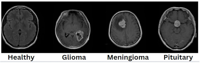
Figure 2: Brain tumor images, including tumor types. The dataset contains four images of healthy brain tissue and three tumorous images: glioma, meningioma, and pituitary. Please click here to view a larger version of this figure.
Proposed model
Following the pre-processing stage, the next step is to suggest a training model effective only for brain tumor classification. For this, it has been proposed an efficient model for training, specifically for classifying brain tumors. For this, a novel and efficient hybrid feature fusion-based pretrained model is proposed, including DenseNet12131,32 and EfficientNetB733, which were used to extract the features from the images, and further, those extracted features were concatenated and passed to different fine-tuned hyperparameters, including trainable and non-trainable layers, to diagnose brain tumors accurately, and have been implemented on five different publicly available datasets, which were discussed in the above related sections. Furthermore, the DenseNet121 model was developed by Gao Huang and his co-workers in 2017 and comprises 121 layers. The main aim of this model was to focus on maximizing feature reuse and avoiding the vanishing gradient problem34. The layers in this model are organized into dense blocks, each containing multiple convolutional layers that extract and learn features. Each layer takes the feature map from all preceding layers as input, and its output is connected to the outputs of those layers and passed as input to subsequent layers in the same block in a feed-forward fashion. Further, transition layers are added between dense blocks, each composed of a 1 × 1 convolutional layer, a BatchNormalization layer, and 2 × 2 average pooling layers, which reduce the feature map to control the model's complexity. Furthermore, a final layer is added with a SoftMax activation function (AF) before a global average pooling layer for classification. The DenseNet121 model's fundamental design is shown in Figure 334 below.
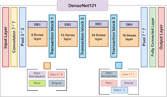
Figure 3: DenseNet121 architectural detail34. This figure shows the architectural detail of the DenseNet121 model, including all dense and transition blocks. Please click here to view a larger version of this figure.
Further, the EfficientNetB7 model was invented by Tan and Lee in 2019. It belongs to the EfficientNet family, with variants from B0 to B7, and its primary goal is to outperform others while using fewer parameters and less processing power. Model width (number of channels per layer), depth (number of layers), and resolution can all be fine-tuned via compound scaling, which is the model's core feature. Further, this model comprises of MBConv (mobile inverted bottleneck convolutional) blocks, which have a 1 × 1 convolutional expansion layer responsible for expanding channels, a depthwise separable convolution that is responsible for applying convolution to each channel separately, and a 1 × 1 convolutional projection layer that reduces the number of channels to the original. Further, each MBConv block consists of Squeeze and Excitation (SE) blocks35, which recalibrate channel-wise features, helping the network focus on the most important ones. Further, instead of sigmoid or any other AF, the Swish function is used, which performs better than ReLU by allowing negative values, which helps in gradient flow. Moreover, a final output layer is added with a SoftMax AF before a global average pooling layer for classification purposes. Figure 435 shows the basic design of the EfficientNetB7 model, whereas Figure 5 shows the recommended model architecture.
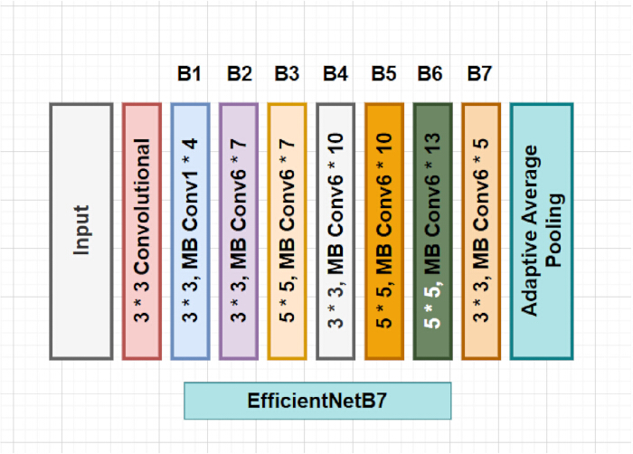
Figure 4: EfficientNetB7 architectural detail35. This figure shows the architectural detail of the EfficientNetB7 model, including all mobile inverted bottleneck convolutional blocks. Please click here to view a larger version of this figure.
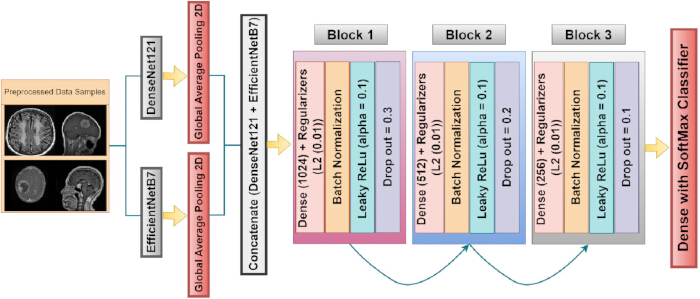
Figure 5: Proposed hybrid fused model architecture. The proposed architecture illustrates how preprocessed images are passed to the feature extractor, which consists of three customized blocks with different hyperparameters, followed by an output layer. Please click here to view a larger version of this figure.
Additionally, first features were extracted from the pretrained DenseNet121 and EfficientNetB7 models. The pretrained models' updated weights were loaded onto the trained models, and it froze the untrainable base layers of the models to prevent the model from being trained again. This should help the model retain its best knowledge from the past, adapt it in light of new data samples to improve convergence, and focus on additional layers to train and extract advanced features. The Below equations 1 and 2 show the workings of the DenseNet121 and EfficientNetB7 models.
 (1)
(1)
 (2)
(2)
The above equations 1 and 2 show the working of the pretrained model regarding feature extraction; F1 denotes the output feature maps produced by the pretrained DenseNet121 model and F2 denotes the output feature maps produced by the pretrained EfficientNetB7 model by applying processing to input images, which is represented by X. further, W1 and W2 are the learnable parameters or weights associated with the first blocks and layers of the DenseNet121 and EfficientNetB7 models, respectively. Further, ∈ RN ×H1×W1×C1 and ∈ RN ×H2×W2×C2 represent the dimensionality of the output feature maps of the DenseNet121, and EfficientNetB7 models, respectively, with dimensions of H1 ×N×W1×C1 and H2 ×N×W2×C2, where N represents the batch size of the images, which was considered 16. Further, H1×W1 represents the height and width of the images, respectively for the DenseNet121 model and H2×W2 represents the height and width of the images for the EfficientNetB7 model and has been selected with 224 × 224 height and width sizes. C1 and C2 represents the color channel for DenseNet121 and EfficientNetB7 models, respectively. After getting output feature maps from the model as 2560 channels output from EfficientNetB7 and 1024 from DenseNet121, the global average pooling 2D36 layer is applied to the output feature maps to reduce the spatial dimension by taking the average of all spatial dimensions to a single vector, which is more convenient to pass to the next layer for better feature extraction and pattern recognition in terms of features that are interpretable.
 (3)
(3)
 (4)
(4)
The above equations 3 and 4 show the workings of the global average pooling 2D layer applied to the DenseNet121 and EfficientNetB7 models, respectively, where  and
and  shows the procedure of normalizing the sum by dividing the total number of spatial locations for both models to ensure that the pooled output is an average rather than a simple sum.
  and
and  represents the summation across the spatial dimensions of the feature maps, while i, and j These are just for iterating over height and width, respectively, to sum the feature maps for both models. Further, F1(i, j, :) and F2(i, j, :) represents the values of feature maps at particular spatial positions (i, j) across all the channels for both DenseNet121 and EfficientNetB7 models, respectively. This pooling operation aggregates spatial information into a more compact and accurate representation while preserving the most important features across every image. Further, the outputs of the global average pooling layers are concatenated to produce a single feature vector for each sample, which is often used to fuse features from different models to improve performance by leveraging both models’ strengths; Equation 5 shows how it works.
![Matrix equation G=[G1,G2]∈ℝN×(C1+C2); linear algebra; mathematical formula; research analysis.](/files/ftp_upload/73365/73365eq5.jpg "figure-protocol-14") (5)
(5)
Above equation 5 shows the concatenation procedure of two different model feature vectors [G1, G2] where G1 represents the features vector of the DenseNet121 model and G2 represents the feature vector of the EfficientNetB7 model, while the shape of the concatenated feature vector is represented by RN ×(C1+ C2), where N is the batch size, which represents the number of samples that proceed in parallel, and (C1+ C2) are the total number of features getting from model 1 and 2 respectively which are about to 3584, which are processed in parallel, and the concatenated output feature vector is represented by G. Further, three different blocks have been added to modify the fused model for extracting more complex features, improving generalization, and preventing overfitting, just to get more accurate and efficient results. Each block is composed of a dense layer with a different number of neurons, and the first block has 1024 neurons in its dense layers, which focus on capturing a wide range of features and more generic patterns in data, while the second block has 512 neurons in its dense layer, which specifically refines the features by reducing dimensionality and focusing on more specific patterns. The third block contains 256 neurons in its dense layer, which are more specifically distilling the features to ensure that only the most relevant features and patterns are passed to the output layer to perform a more relevant task. Further, L2 regularization37 approaches are added to every dense layer in each block to prevent overfitting by penalizing larger weights, and this is also causing the model to become more complex. A dropout layer38 is also introduced after each block just to randomly ignore 30%, 20%, and 10% of neurons for blocks 1, 2, and 3, respectively, which forces networks to develop more robust features that are not reliant on a single neuron. Further, to stabilize the training process, a BatchNormalization39 layer is applied after each dense layer, which ensures that the activations remain within a stable range and also helps the model to avoid issues like vanishing gradients and exploding gradients during the training phase. Additionally, this BatchNormalization layer also accelerated the training process, which allowed the model to converge faster by smoothing the loss landscape, which made it easier to get global minima for optimizers. Further, in each block, to produce non-linearity, leaky ReLU activation40 is used, which allows the model to learn complex patterns, and leaky ReLU has advantages over other activation functions that ensure that the neuron doesn’t become inactive by allowing a small, non-zero gradient for negative inputs. Further, the below equation 6 show the working of different blocks integrated with the hybrid fused model.
 (6)
(6)
After getting the concatenated vector, G is passed through the block 1 dense layer (fully connected) with 1024 neurons, where the weight matrix W1 transforms the input vector G into a 1024-dimensional output vector and each element in output vector is a linear combination of the input features. Further, the b1 bias vector is then added to each of the 1024 elements in the output, which allows the model to shift the output of the input features independently. Further, the L2 regularization term: λ||W1||22 penalizes the large weights, which discourages the model from depending excessively on a single neuron, which helps to avoid overfitting. Where, the weight matrix of a particular layer is W1 in the neural network, while ||W1||22 denotes the squared L2 norm of the weight matrix W1 and λ is the regularization parameter that controls the degree of regularization applied, which has been set to 0.1 in all blocks. Z1 Become the new feature representation after applying the dense layer as well as L2 regularization on the input passed from the concatenated vector G, which is shown in equation 6.
After getting output from the dense layer of block 1 as Z1, the BatchNormalization layer was applied, which was used to speed up the training process, and the below equation 7 shows how it works.
 (7)
(7)
σ2 Represents the variance of the output of the last layer Z1 across the batch, while μ is the mean of the output Z1 which is calculated separately for each neuron, which was 1024 in the first dense layer. While, ε is a minor constant that is incorporated to ensure numerical stability and prevent division by zero. The normalized output can be adjusted by the model by adjusting the learnable scale parameter γ, while the normalized output can be shifted by the learnable shift parameter β. Finally, after applying the BatchNormalization layer to the output of the dense layer, the normalized output Z1, ensures that the activations have a consistent distribution over the different layers, which helps to stabilize and speed up training. After the BatchNormalization the normalized output Z1 passed through the leaky ReLu activation function, which produces non-linearity in the network which helps to learn complex patterns in the data. Instead of choosing ReLU or another activation function, leaky ReLU were chosen, which is the modified version of ReLU function that considers small negative values also instead of making them 0 like ReLU activation function as overcome the dying ReLU problem. Equation 8 below shows how it works.
 (8)
(8)
Where Z1 belongs to the output of BatchNormalization layer, which is passed to Leaky ReLU as input for performing non-linearity, while ∝ is a small constant that is used to determine the slope of the negative part of the function. Further, A1 shows the output that is obtained after applying non-linearity. Finally, a dropout layer is applied to the output A1 received as input from Leaky ReLu activation, which is shown in the equation 9.
 (9)
(9)
Where A1 is the original activation function output received from the last ReLu activation function, and where p is the dropout rate, which varies between 0 and 1 and has been selected as 0.3, 0.2, and 0.1 for three block layers, respectively, just for dropping the fraction of neurons. Further, A1′ shows the modified output after applying the dropout layer, from which some neurons have set to 0. The main advantage of using it is just to prevent the overfitting issues as well as reducing co-adaptation. Further, the output from block1 A1′ passed to the next block again for extracting more abstract features again and applied the same parameters that are in block 1, with some distinguishing of 512 neurons in the dense layer instead of 1024 and a dropout rate of 0.2 instead of 0.3, and the other operational sequences are the same, which is described in the below equations 10 to 13.
 (10)
(10)
 (11)
(11)
 (12)
(12)
 (13)
(13)
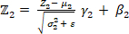
After getting the output from block 1 as, A1′ which is passed through the block 2 dense layer (fully connected) with 512 neurons, where the weight matrix W2 transforms the input vector A1′ into a 512-dimensional output vector, and each element in the output vector is a linear combination of the input features. Further, the b2 bias vector is then added to each of the 512 elements in the output, which allows the model to shift the output of the input features independently. Further, the L2 regularization also applied where: λ||W2||22 penalized the large weights, which serves to mitigate overfitting by preventing the model from placing an excessive amount of reliance on any particular neuron in this specific block. Where, W2 is the weight matrix of a particular layer in the neural network, while, λ is the regularization parameter that controls the degree of regularization applied that has been applied as 0.1. Z2 Become the new feature representation after applying the dense layer as well as L2 regularization on input passed from block 1, which is shown in equation 10.
Further, the BatchNormalization layer was applied to the new feature Z2, which was used to speed up the training process, σ22 Represents the variance across the batch, while μ2 is the mean of the output Z2. Although ε is a small constant that is incorporated to ensure numerical stability, γ is a learnable scale parameter that enables the model to modify the normalized output, and β is a learnable shift parameter that enables the model to shift the normalized output. Finally, after applying the BatchNormalization layer, which is shown in equation 11, the normalized output Z2 passed through the leaky ReLU AF, which produced non-linearity in the network, which is shown in equation 12. Where Z2 belongs to the output of the BatchNormalization layer, which passes to Leaky ReLU as input for performing non-linearity. While, A2 shows the output that is obtained after applying non-linearity.
Finally, a dropout layer is applied to the output A2 received as input from Leaky ReLU activation, which is shown in equation 13. Where A2 is the output received from the last ReLU activation function, and where p2 is the dropout rate, which has been selected 0.2 for this block, just for dropping the fraction of neurons. Further, A2′ shows the modified output after applying the dropout layer, from which some neurons have set to 0. Further, the output from block 2 A2′ passed to the third block again for extracting again more abstract features and applied the same parameters that are in block 2, with some distinguishing of 256 neurons in the dense layer instead of 512 and a dropout rate of 0.1 instead of 0.2, and the other operational sequences are same, which is described in the below equations 14 to 17.
 (14)
(14)
 (15)
(15)
 (16)
(16)
 (17)
(17)
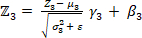
After getting the output from block 2 as, A2′ which is passed through the block 3 dense layer (fully connected) with 256 neurons, where the weight matrix W3 transforms the input vector A2′ into a 256-dimensional output vector, and each element in the output vector is a linear combination of the input features. Further, the b3 bias vector is then added to each of the 256 elements in the output, which allows the model to shift the output of the input features independently. Further, the L2 regularization also applied where: λ||W3||22 penalized the large weights, which discourages the model from depending excessively on a single neuron, which helps to avoid overfitting. Where, W3 is the weight matrix of a particular layer in the neural network, while, the degree of regularization employed is controlled by the regularization parameter λ , which has been set to 0.01. Z3 Become the new feature representation after applying the dense layer as well as L2 regularization on input passed from block 3, which is shown in equation 14.
Further, the BatchNormalization layer was applied to the new feature Z3, which was used to speed up the training process, σ32 Represents the variance across the batch, while μ3 is the mean of the output Z3. While, ε is the small constant that is added for numerical stability. The normalized output can be adjusted by the model using the learnable scale parameter γ3, and shifted using the learnable shift parameter β3. Finally, after applying the BatchNormalization layer, which is shown in equation 15, the normalized output Z3 passed through the leaky ReLU activation function, which produced non-linearity in the network, which is shown in equation 16. Where Z3 belongs to the output of the BatchNormalization layer, which passes to Leaky ReLU as input for performing non-linearity. While, A3 shows the output that is obtained after applying non-linearity.
Finally, a dropout layer is applied to the output A3 received as input from Leaky ReLU activation, which is shown in equation 17. Where A3 is the output received from the last ReLU activation function, and where p3 is the dropout rate, which has been selected 0.1 for this block, just for dropping the fraction of neurons. Further, A3′ shows the modified output after applying the dropout layer, from which some neurons have set to 0.
Further, the output from block 3 A3′ passed through the last dense layer for classification purposes with a K number of neurons that represents the actual number of classes in the dataset, which is described in equation 18 below.
 (18)
(18)
The weight matrix linked to the thick layer is Wk, which is responsible for transforming the 256-dimensional vector A3′ into k-dimensional vector, which represents the learned features from the previous block and comes as output. Further, bk represents the bias vector that adjusts the prediction to ensure that the activation function has a non-zero output when the input is zero, and Zk is the output of the final layer before applying the activation function, and it produces the logits against each class, and in the last SoftMax41 classifier has been applied that converts the logit Zk into the probability of each class, which is shown in equations 19 and 20.
 (19)
(19)
 (20)
(20)
Where the predicted probability of the ith class is represented by yi, K is the number of classes, while Zk, i is the logit for the ith class, and eZk, i is the exponential of the logit of ith class. y shows the probability distribution of all possible classes and ensures the sum of probabilities is 1. Table 3 below provides the hyperparameter details used to train the proposed hybrid model, including the architectural details adopted for improved reproducibility and performance.
| Hyper Parameters | Proposed Model (FusionNetX) |
| Image size | 224 × 224 |
| Backbone Architecture | Pretrained EfficientNetB7 and DenseNet121 as BBA1, and BBA2 |
| Data Augmentation | Rotation range = 7, |
| Width/height – shift range up to 0.05, | |
| Zoon range up to 0.01, | |
| Horizontal/vertical – flip | |
| Data splitting ratio | 80% for training and 20% for validation on stratified sampling with fixed randome_state = 42 |
| Feature extraction and fusion | Global average pooling is applied on each backbone’s output: 2560 for BBA1 and 1024 for BBA2 and fused to get 3584 joint feature vectors. |
| Fully Connected Block Composition | 3 fully connected blocks with 1 output layer. Each block contains L2 regularization (λ=0.01), BatchNormalization, LeakyReLU (α=0.01), Dropout of (0.3, 0.2, and 0.1) and hidden dimension of (1024, 512, 256) respectively. No additional Skip connection introduced in fusion head |
| Activation function | Leaky ReLU & SoftMax |
| Optimizer and Learning rate | Adam with 0.00001 fixed with no learning rate scheduler. |
| Loss function | sparse_categorical_crossentropy |
| Batch size | 16 |
| Epochs | 100 fixed epochs for each dataset |
| Plateform used | Kaggle Notebook having a P100 GPU and 16GB VRAM with the TensorFlow and Keras platforms. |
Table 3: Hyperparameters used to train the proposed model and proposed architectural details. This table provides the structural and architectural details of the proposed model, along with fine-tuned parameters and implementation environment.
Access restricted. Please log in or start a trial to view this content.
Results
This part details the results of testing the proposed dual feature fusion model on five open-source datasets on brain cancers, including Br35H, Figshare, Sartaj, Masoud, and Balanced Brain tumor datasets, and their performance is evaluated regarding different statistical performance evaluation parameters, including accuracy42,43,44, misclassification rate (MCR)45, precision, also referred as PPV
Access restricted. Please log in or start a trial to view this content.
Discussion
As concluded, the proposed model worked as follows: First, the image size was chosen as 224 × 224, which is the moderate size for any deep learning model to extract and learn suitable features from the data samples while keeping all important information, and further performed data augmentation, which is more beneficial to make data samples in more diverse directions, which plays an important role for models to extract features from different planes or angles, and the rotational range was selected as 7% with a width...
Access restricted. Please log in or start a trial to view this content.
Disclosures
The authors have nothing to disclose and have no conflict of interest. Further, no AI tools have been used to generate the manuscript as well as figures.
Acknowledgements
The authors are grateful for the support provided by the Princess Nourah bint Abdulrahman University Researchers Supporting Project (PNURSP2026R192), Princess Nourah bint Abdulrahman University, Riyadh, Saudi Arabia. The authors also thank the research participants and institutions that contributed to this research.
Funding:
This work was supported by the National Research Foundation of Korea (NRF) grant funded by the Korea government (MSIT) (No. RS-2023-00218176) and the Soonchunhyang University Research Fund. Princess Nourah bint Abdulrahman University Researchers Supporting Project number (PNURSP2026R192), Princess Nourah bint Abdulrahman University, Riyadh, Saudi Arabia.
Access restricted. Please log in or start a trial to view this content.
Materials
| Name | Company | Catalog Number | Comments |
|---|---|---|---|
| Br35H Brain Tumor Dataset | Kaggle (dataset contributor) | https://www.kaggle.com/datasets/ahmedhamada0/brain-tumor-detection | Public dataset; binary classification (tumor / no tumor)300 MRI images |
| Figshare Brain Tumor Dataset | Kaggle / Figshare | https://doi.org/10.6084/m9.figshare.1512427 | Public dataset; multiclass (glioma, meningioma, pituitary tumor) 3064 MRI images |
| Sartaj Brain Tumor Classification MRI Dataset | Kaggle (dataset by Sartaj Bhuvaji) | https://doi.org/10.34740/kaggle/dsv/12745533 | Public dataset; multiclass (glioma, meningioma, no tumor, pituitary tumor) 3264 MRI images |
| Masoud Brain Tumor MRI Dataset | Kaggle (dataset by Masoud Nickparvar) | https://doi.org/10.34740/kaggle/dsv/14832123 | Public dataset; multiclass (glioma, meningioma, no tumor, pituitary tumor) 7023 MRI images |
| BBT-Dataset (Brain Tumor Dataset) | Kaggle (dataset contributor) | https://doi.org/10.34740/kaggle/dsv/6758053 | Public dataset; balanced multiclass brain tumor 5248 MRI images |
| Python | Python Software Foundation | https://www.python.org | Programming language, version 3.10.13 |
| TensorFlow / Keras | Google / TensorFlow developers | https://www.tensorflow.org | Deep learning framework; model construction, training, and evaluation, version 2.15.0 |
| EfficientNetB7 (pretrained) | Google / Keras Applications | https://keras.io/api/applications/efficientnet/ | ImageNet-pretrained backbone; feature extraction |
| DenseNet121 (pretrained) | Keras Applications | https://keras.io/api/applications/densenet/ | ImageNet-pretrained backbone; feature extraction |
| scikit-learn | scikit-learn developers (NumFOCUS) | https://scikit-learn.org | Label encoding, train-test split, evaluation metrics (classification report, confusion matrix, ROC/AUC) |
| OpenCV (cv2) | OpenCV team | https://opencv.org | Image loading and resizing |
| NumPy | NumPy developers (NumFOCUS) | https://numpy.org | Numerical computing and array operations |
| pandas | pandas development team (NumFOCUS) | https://pandas.pydata.org | Data organization and metrics tabulation |
References
- He Z, et al. A review on methods for diagnosis of breast cancer cells and tissues. Cell Prolif. 2020;53(7):e12822. doi:10.1111/cpr.12822.
- Siegel RL, Giaquinto AN, Jemal A. Cancer statistics, 2024. CA Cancer J Clin. 2024;74(1):12–49.
- Varuna Shree N, Kumar TNR. Identification and classification of brain tumor MRI images with feature extraction using DWT and probabilistic neural network. Brain Inform. 2018;5(1):23–30.
- Ghoreishi Mokri SM, Valadbeygi N, Grigoryeva V. Diagnosis of glioma, menigioma and pituitary brain tumor using MRI images recognition by deep learning in Python. EAI Endorsed Trans Intell Syst Mach Learn Appl. 2024;1:1–9.
- Sadeghi MH, et al. Deep learning in ovarian cancer diagnosis: a comprehensive review of various imaging modalities. Pol J Radiol. 2024;89:e30–e48.
- Anari S, Safarpour H, Cunneen M, Bendechache M. AR-EpiAid: an augmented reality decision support system for real-time interpretation of multimodal epilepsy data [conference paper]. Presented at: 3rd International Conference on Artificial Intelligence, Computer, Data Sciences, and Applications; Boracay Island, Philippines; 2026. https://doi.org/10.1109/ACDSA67686.2026.11468245.
- Iyortsuun NK, et al. A review of machine learning and deep learning approaches on mental health diagnosis. Healthcare (Basel). 2023;11(3):285. doi:10.3390/healthcare11030285.
- An Q, Rahman S, Zhou J, Kang JJ. A comprehensive review on machine learning in the healthcare industry: classification, restrictions, opportunities, and challenges. Sensors (Basel). 2023;23(9):4178. doi:10.3390/s23094178.
- Iqbal S, Qureshi AN, Li J, Mahmood T. On the analyses of medical images using traditional machine learning techniques and convolutional neural networks. Arch Comput Methods Eng. 2023;30:3173–3233.
- Chhimpa GR, et al. A transfer learning-driven fine-tuning of YOLOv10 for improved brain tumor detection in MRI images. Sci Rep. 2026;16:98. doi:10.1038/s41598-025-28813-w.
- Akbarian S, Seyyed-Kalantari L, Khalvati F, Dolatabadi E. Evaluating knowledge transfer in the neural network for medical images. IEEE Access. 2023;11. doi:10.1109/ACCESS.2023.3283216.
- Meena G, Mohbey KK, Acharya M, Lokesh K. An improved convolutional neural network-based model for detecting brain tumors from augmented MRI images. J Auton Intell. 2023;6:1–19.
- Ata MM, Yousef RN, Karim FK, Khafaga DS. An improved deep structure for accurately recognizing brain tumors. Comput Syst Sci Eng. 2023;46(2):1597–1616.
- Khushi HMT, et al. Performance analysis of state-of-the-art CNN architectures for brain tumour detection. Int J Imaging Syst Technol. 2024;34:e22949. doi:10.1002/ima.22949.
- Agarwal M, et al. Deep learning for enhanced brain tumor detection and classification. Results Eng. 2024;22:102117. doi:10.1016/j.rineng.2024.102117.
- Peddinti AS, Maloji S. Optimised ResNet50 for multiclass classification of brain tumors. Scalable Comput Pract Exp. 2024;25(3):1667–1680.
- Zahoor MM, et al. Brain tumor MRI classification using a novel deep residual and regional CNN. Biomedicines. 2024;12(7):1395. doi:10.3390/biomedicines12071395.
- Chen W, et al. A robust approach for multitype classification of brain tumors using deep feature fusion. Front Neurosci. 2024;18:1288274. doi:10.3389/fnins.2024.1288274.
- Suryawanshi S, Patil SB. Efficient brain tumor classification with a hybrid CNN-SVM approach in MRI. J Adv Inf Technol. 2024;15:340–354.
- Reyes D, Sánchez J. Performance of convolutional neural networks for the classification of brain tumors using magnetic resonance imaging. Heliyon. 2024;10:e25468. doi:10.1016/j.heliyon.2024.e25468.
- Bibi N, et al. A transfer learning-based approach for brain tumor classification. IEEE Access. 2024;12:111218–111238.
- Albalawi E, et al. Integrated approach of federated learning with transfer learning for classification and diagnosis of brain tumor. BMC Med Imaging. 2024;24:110. doi:10.1186/s12880-024-01261-0.
- Alkhatib AJ, et al. Diagnosing brain tumors from MRI images through a multi-fused CNN with auxiliary layers. Sustain Mach Intell J. 2024;6(1):4–13.
- Hamada A. Br35H: Brain Tumor Detection 2020 [dataset]. Kaggle; 2020. Available from: https://www.kaggle.com/datasets/ahmedhamada0/brain-tumor-detection.
- Cheng J. Brain tumor dataset [dataset]. Figshare; 2024. Available from: https://doi.org/10.6084/m9.figshare.1512427.
- Bhuvaji S. Brain Tumor Classification (MRI) [dataset]. Kaggle; cited 2026 Jul 30. Available from: https://doi.org/10.34740/kaggle/dsv/12745533.
- Nickparvar M. Brain Tumor MRI Dataset [dataset]. Kaggle; cited 2026 Jul 30. Available from: https://doi.org/10.34740/kaggle/dsv/14832123.
- Jayanti V. Brain Tumor MRIs [dataset]. Kaggle; cited 2026 Jul 30. Available from: https://doi.org/10.34740/kaggle/dsv/6758053.
- Tuteja P, et al. Augmented multimodal fusion for optimized brain tumor detection: evaluation and comparative analysis. J Vis Exp. 2025;(220):e67822. doi:10.3791/67822.
- Rasool N, et al. CNN-TumorNet: leveraging explainability in deep learning for precise brain tumor diagnosis on MRI images. Front Oncol. 2025;15:1554559. doi:10.3389/fonc.2025.1554559.
- Huang G, Liu Z, van der Maaten L, Weinberger KQ. Densely connected convolutional networks [conference paper]. Presented at: IEEE Conference on Computer Vision and Pattern Recognition; Honolulu, HI, USA; 2017. p. 4700–4708. Available from: https://openaccess.thecvf.com/content_cvpr_2017/html/Huang_Densely_Connected_Convolutional_CVPR_2017_paper.html.
- Tuteja P, Wani MA, Wani NA, Bedi J. EASE-Net: an explainable AI-based segmentation and ensemble network for interpretable brain tumor diagnosis and classification in MRI images. Arab J Sci Eng. 2026;in press. doi:10.1007/s13369-026-11350-7.
- Tan M, Le QV. EfficientNet: rethinking model scaling for convolutional neural networks [conference paper]. Presented at: 36th International Conference on Machine Learning; Long Beach, CA, USA; 2019. p. 6105–6114. Available from: https://proceedings.mlr.press/v97/tan19a.html.
- Vellaichamy AS, Swaminathan A, Varun C, Kalaivani S. Multiple plant leaf disease classification using DenseNet-121 architecture. Int J Electr Eng Technol. 2021;12(5):38–57.
- Naidji MR, Elberrichi Z. Automatic detection of COVID-19 from chest X-ray images using the EfficientNet-B7 CNN model with channel-wise attention. Int J Comput Digit Syst. 2024;15:1443–1456.
- Malla PP, Sahu S, Alutaibi AI. Classification of tumors in brain MR images using a deep convolutional neural network and global average pooling. Processes. 2023;11(3):679. doi:10.3390/pr11030679.
- Shi G, Zhang J, Li H, Wang C. Enhance the performance of deep neural networks via L2 regularization on the input of activations. Neural Process Lett. 2019;50:57–75.
- Srivastava N, et al. Dropout: a simple way to prevent neural networks from overfitting. J Mach Learn Res. 2014;15:1929–1958.
- Ioffe S, Szegedy C. Batch normalization: accelerating deep network training by reducing internal covariate shift [conference paper]. Presented at: 32nd International Conference on Machine Learning; Lille, France; 2015. p. 448–456. Available from: https://proceedings.mlr.press/v37/ioffe15.html.
- Varshney M, Singh P. Optimizing nonlinear activation functions for convolutional neural networks. Signal Image Video Process. 2021;15:1323–1330.
- Bera S, Shrivastava VK. Analysis of various optimizers on a deep convolutional neural network model in the application of hyperspectral remote-sensing image classification. Int J Remote Sens. 2020;41:2664–2683.
- Safarpour H, et al. A dual-phase segmentation framework utilizing Gumbel-Softmax and a cascaded Swin Transformer for multiclass brain tumor segmentation. Research Square. 2025:doi:10.21203/rs.3.rs-7093467/v1.
- Seyrek EC, Uysal M. A comparative analysis of various activation functions and optimizers in a convolutional neural network for hyperspectral image classification. Multimed Tools Appl. 2024;83:53785–53816.
- Maxwell AE, Warner TA, Guillén LA. Accuracy assessment in convolutional neural network-based deep-learning remote-sensing studies—part 1: literature review. Remote Sens (Basel). 2021;13(13):2450. doi:10.3390/rs13132450.
- Villon S, et al. A new method to control error rates in automated species identification with deep-learning algorithms. Sci Rep. 2020;10:10972. doi:10.1038/s41598-020-67573-7.
- Rasool N, et al. TransResUNet: revolutionizing glioma brain tumor segmentation through transformer-enhanced residual UNet. IEEE Access. 2024;12:72105–72116.
- Chen Y, et al. Evaluation efficiency of hybrid deep-learning algorithms with neural-network decision-tree and boosting methods for predicting groundwater potential. Geocarto Int. 2022;37:5564–5584.
- Alakus TB, Turkoglu I. Comparison of deep-learning approaches to predict COVID-19 infection. Chaos Solitons Fractals. 2020;140:110120. doi:10.1016/j.chaos.2020.110120.
- Ranjbarzadeh R, et al. Explainable attention-guided Swin Transformer networks for brain tumor segmentation from 3D MRI. Lect Notes Netw Syst. 2026;1730:110–128. Available from: https://lero.ie/bibliography/explainable-attention-guided-swin-transformer-networks-for-brain-tumor-segmentation-from-3d-mri/.
- Ranjbarzadeh R, et al. A global-local 3D brain tumor segmentation model using vision transformers and axial state-space modeling [conference paper]. Presented at: 3rd International Conference on Artificial Intelligence, Computer, Data Sciences, and Applications; Boracay Island, Philippines; 2026. https://doi.org/10.1109/ACDSA67686.2026.11468214.
- Hussain SS, et al. Next-generation automation in neuro-oncology: advanced neural networks for MRI-based brain tumor segmentation and classification. IEEE Access. 2025;13:41141–41158.
Access restricted. Please log in or start a trial to view this content.