Enrichment of Retinal Endothelial Cells and Müller Glia Enable Comprehensive scRNA-Seq Profiling of the Blood-Retinal Barrier

Summary

Analysis of low-abundant target cell populations remains a challenge, even with high-throughput omics. Here, we describe techniques to selectively enrich for target cell types from complex retinal tissue while preserving the general cell heterogeneity.

Abstract

Obtaining high-quality single-cell suspensions from neural tissues such as the murine retina remains technically challenging due to cellular fragility, tight intercellular junctions, and the heterogeneous composition of the tissue. These challenges are further compounded when studying rare cell populations, including vascular endothelial cells and Müller glia, which each account for less than 2% and are underrepresented in standard dissociation workflows, often lost during processing. Here, we present an optimized method for isolating murine retinal cells that preserves cellular integrity and enables selective enrichment of sparse populations for downstream single-cell RNA sequencing (scRNA-seq).

Our protocol integrates gentle enzymatic dissociation with mechanical trituration to maximize cell viability and minimize transcriptional artifacts. We further incorporate targeted enrichment strategies, using fluorescence-activated cell sorting (FACS), to increase the relative abundance of vascular endothelial and Müller glial cells without compromising overall transcriptomic diversity. Moreover, we tested antibody-based cell hashing to enable sample multiplexing to improve cost efficiency. We demonstrate that this approach yields high-quality single-cell suspensions with improved representation of rare retinal cell types, enabling more robust and reproducible scRNA-seq analyses. This method provides a practical framework for researchers aiming to investigate the vascular and glial cell components of the retina at single-cell resolution and can be adapted to other neural tissues in which rare cell populations are of interest.

Introduction

The retina is a highly specialized neurovascular tissue composed of diverse neuronal, glial, and vascular cell populations that function in close coordination to enable visual perception. Among these populations, retinal vascular endothelial cells (ECs) and Müller glia play essential roles in maintaining the integrity of the inner blood–retina barrier¹. However, both cell types are present only in low abundance within the murine retina, with ECs accounting for approximately 0.6%² of total retinal cells and Müller glia representing approx. 1.5%³. The scarcity of these cells presents a substantial technical challenge for downstream transcriptomic analyses, particularly for single-cell RNA sequencing (scRNA-seq), where insufficient enrichment may result in inadequate sampling and loss of biologically relevant information.

Recent studies have demonstrated that Müller glia and ECs closely interact to regulate retinal barrier permeability and vascular stability¹. This cellular crosstalk is essential for maintaining retinal homeostasis under physiological and pathological conditions. Consequently, the simultaneous isolation, enrichment, and characterization of these rare retinal populations within the diverse retinal cell environment is of considerable interest for understanding neuro-glio-vascular interactions in the retina at single-cell resolution.

Fluorescence-activated cell sorting (FACS) presents a successful approach for the selective enrichment of rare cell populations from heterogeneous tissues⁴. In order to utilize this approach, cell surface markers must be present to securely label different cell types, therefore forcing researchers to abandon otherwise performed single-nuclei sequencing. Especially in fragile neuronal tissues, usually single-nuclei sequencing is preferred due to its robustness, while single-cell sequencing presents a challenge when trying to sample highly viable cells for downstream analysis.

By using highly specific cell-surface markers, our FACS-based approach enables efficient isolation of sparse cell populations while still sampling viable single cells suitable for downstream molecular applications. In the murine retina, GLAST1 has been described as a selective membrane-associated marker for Müller glia⁵, while CD31+ CD45- staining is widely used as a specific marker for endothelial cells⁶. The combination of these markers provides an opportunity for targeted enrichment of both retinal cell populations while preserving cellular diversity within the tissue.

Antibody-based cell hashing provides an opportunity to enable sample multiplexing, therefore reducing the cost per experiment. Using antibody-linked RNA probes, major histocompatibility complex 1 (MHC1)-based hashing binds to all cells expressing MHC1 on the cellular membrane, which leads to incorporation of the Probes into the sequenced transcriptome, therefore allowing for downstream sample demultiplexing⁷.

A critical requirement for successful scRNA-seq is the preservation of high-quality, intact single cells throughout tissue dissociation and sorting procedures⁸. Excessive manipulation or prolonged processing can induce transcriptional artifacts, reduce cell viability, and compromise the representation of native cellular heterogeneity. Therefore, optimized enrichment strategies are necessary to isolate rare retinal populations while minimizing technical bias and preserving the physiological transcriptional state of individual cells.

In this study, we established a selective FACS-based enrichment workflow for murine retinal ECs and Müller glia using CD31 and GLAST1 as cell-specific markers. To prevent the false identification of CD31+/CD45+ cells as ECs, we initially performed CD31/CD45 co-staining and conducted FACS analysis. In mouse tissue, however, we did not encounter CD31/CD45 double-positive cells that could have been mistakenly identified as ECs. This approach aimed to enrich low-abundance retinal cell populations while preserving a high-quality single-cell suspension suitable for downstream single-cell RNA sequencing analyses without loss of retinal cellular heterogeneity.

Protocol

All mouse experiments adhered to the animal care guidelines of the Institute for Laboratory Animal Research (Guide for the Care and Use of Laboratory Animals) in accordance with both the Animal research: Reporting of in vivo experiments (ARRIVE) guidelines and the association for research in vision and ophthalmology (ARVO) statement for the use of animals in ophthalmic and vision research. Experiments were approved by the local animal welfare committee (Tierschutzkommission) under approval number G22-053.

Pregnant C57BL/6J mice were obtained from Janvier Labs. Six pups were euthanized on postnatal day 13 (P13). Three mice (i.e., biological replicates) were used per treatment group, and both retinas from one mouse were pooled per sample. Between treatment groups, mice were not controlled or matched for sex. Notably, the protocol was also tested on 17-day-old and adult mice. The reported protocol was conducted multiple times to ensure reproducibility.

1. Experimental setup

1. Determine treatment groups.
2. Use at least 3 mice per treatment group (= biological replicates)
3. Include control samples: unstained control and fluorescence minus one controls.
4. Depending on the number of animals needed, start breeding or order pregnant mice.
5. Consider the use of hashing antibodies to run all biological replicate samples in one lane for scRNA seq analysis.

2. Preparation of reagents and equipment

1. Preparation of 500 mL of wash buffer:
   1. Prepare 500 mL of PBS, 2 mM ethylenediaminetetraacetic acid (EDTA), 0.25% bovine serum albumin (BSA).
   2. Weigh 0.25 g of Mg²⁺, Ca²⁺ free BSA
   3. Prepare 2 mL of 500 mM Mg²⁺, Ca²⁺ free EDTA Stock
   4. Fill it up to approx. 450 mL with Mg²⁺, Ca²⁺ free PBS, and shake it well.
   5. Adjust pH to 7.2 while stirring.
   6. Top it up to 500 mL while stirring.
   7. Put in fridge at 4 °C overnight.
2. Preparation of coated tubes
   1. Coat 1.5 mL low-binding tubes with BSA stock solution (diluted 1:5 in PBS).
   2. Put in fridge at 4 °C overnight.

3. Extraction of the mouse retina

1. Use at least three mice per group to obtain six eyes per group, and use one additional mouse as an unstained control.
   NOTE: If the litter is too small, use the mother mouse as an unstained control.
2. Perform cervical dislocation followed by induction of anesthesia using isoflurane (3%).
3. Immediately enucleate both eyes by pushing a pair of forceps down next to the eye.
   Extract the eye from the socket
4. Transfer to Hank’s Balanced Salt Solution (HBSS; 1000 µL) and place it on ice.
5. Repeat steps 3.1–3.4 for all mice.
6. Transfer to a backlit microscope.
7. Use forceps, grab the eye at the cornea, and tear open the eye.
8. Peel retina and lens through the prongs of forceps to remove the sclera/choroidal complex.
9. Remove remaining parts of choroid, pigmented cells, and lens.

4. Preparation of single cell suspension

1. Mix Papain (500 µL) + DNase Mix (50 µL) and preheat using a 37 °C water bath (no more than 15 min prior to usage).
2. Transfer both isolated retinae of one mouse to a preheated Papain (500 µL) + DNase mix (50 µL) (in water bath, approx. 37 °C).
3. Incubate for 10 min at room temperature.
4. Break up retinae using a 1000 µL pipette until no clumps are visible.
5. Pipette solution onto albumin-ovomucoid inhibitor solution (500 µL) to stop the reaction.
6. Centrifuge at 1000 × g for 10 min 4 °C.
7. Remove the supernatant.
8. Resuspend the pellet in 1 mL of wash buffer, then transfer it into 5 mL FACS tube, and place on ice.

5. FACS preparation and staining

1. Centrifuge cells in a 5 mL FACS tube at 500 × g for 5 min at 4 °C.
   1. For unstained control, decant the supernatant, resuspend in 300 µL of wash buffer, and place on ice.
2. Decant the supernatant, resuspend in 1000 µL of 1:10.000 (diluted in wash buffer) DAPI for 5 min in the fridge, cover in silver foil to block light.
3. Centrifuge the cells in the FACS tube at 500 × g for 5 min at 4 °C.
4. Decant the supernatant, resuspend in 150 µL of 1:200 Fc Block (CD16/CD32, diluted in wash buffer) for 20 min in the refrigerator, cover in silver foil to block light.
5. Add 1 mL of wash buffer, centrifuge the cells in the FACS tube at 500 × g for 5 min at 4 °C.
6. Decant the supernatant, resuspend in 150 µL of 1:100 CD31-phycoerythrin (PE) and 1:50 Glast-allophycocyanin (APC) (diluted in wash buffer), add 3 µL (0.5 mg/mL) hashing antibody to each condition, and stain for 20 min in the fridge, cover in silver foil to block light.
7. Add 1 mL of wash buffer, centrifuge cells in the FACS tube at 500 × g for 5 min at 4 °C.
8. Wash again with 1 mL of wash buffer, centrifuge cells in the FACS tube at 500 × g for 5 min at 4 °C.
9. Resuspend in 300 µL of wash buffer and proceed with the FACS analysis.
10. Pass through a 30 µm cell strainer immediately before the FACS analysis.
    NOTE: Sorter: benchtop multi-laser fluorescence-activated cell sorter (FACS) equipped with avalanche photodiode (APD)-based detection, electrostatic droplet sorting, and multiparametric digital acquisition for high-sensitivity single-cell analysis and isolation.

6. Flowcytometry set-up and sort

1. Establish cytometer settings using an unstained control to adjust for cell size and granularity.
2. Use fluorescence minus one (FMO) stained control samples to perform compensation set-up.
3. Set gates according to individual compensation, differentiating between negative and positive-stained cells.
4. Sort 50,000 DAPI-negative cells into one coated 1.5 mL low-binding tube (wash buffer).
5. Sort the rest for either CD31-PE or GLAST-APC in separate coated 1.5 mL low-binding tubes and set the threshold at 3,000 cells per mouse (wash buffer).
6. Continue straight with downstream analysis. When analyzing consecutive samples, store on ice for a maximum of 3 h.
7. Determine cell counts per microliter (µL) and load cells according to the experimental setup.
   NOTE: Here, a ratio of 3:1:1 (DAPI negative cells, ECs, and Müller cells, respectively) was used for further single-cell analysis

7. Single-cell library preparation

1. Pool samples for 10x Genomics Library preparation in accordance with the preplanned sequencing strategy and load for drop-seq preparation.
   NOTE: Here, 8,000 cells were loaded. Verify MHC hashing success to avoid uncertainty in post-sequencing sample identification.
2. Process sorted retinal cells through the 10x Genomics single-cell 3′ workflow according to the manufacturer’s instructions⁹.

8. Sequencing

1. Pool libraries to the desired quantities to obtain appropriate sequencing depths as recommended by 10x Genomics and sequenced on a NovaSeq 6000 flow cell⁹.

9. Data analysis

1. Analyze scRNA-seq data using the R package (v4.5.1)¹⁰ and Seurat (v5.4.0)¹¹.
2. Set normalization method to LogNormalize.
3. Perform dimensionality reduction using the RunUMAP function, use the default resolution for clustering.
4. Characterize clusters, differential gene expression analysis using the FindMarkers
   function in Seurat⁹.

Results

Using the workflow described above (Figure 1), we routinely obtain highly viable single‑cell suspensions containing approximately 3–5 million cells per mouse aged 13 days (two pooled retinae) (Figure 2).

Figure 1: Graphical abstract showing the workflow. Single-cell digestion, staining, selective enrichment using flow cytometry, library preparation, sequencing, and subsequent data analysis. Please click here to view a larger version of this figure.

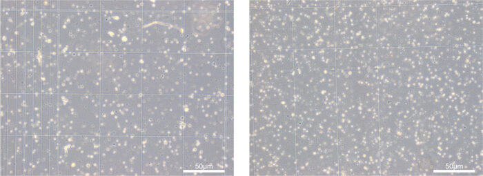
Figure 2: Single cell suspension. Representative images from separate experiments, showing pooled retinae from one mouse each. Scale bar: 50 µm. Please click here to view a larger version of this figure.

This protocol has also been successfully applied to younger mice (from 12 days onward) up to fully adult animals, demonstrating its robustness across developmental stages and tissue maturities.

Following dissociation, we reliably stain and sort target populations using established marker genes. In the present study, CD31 was used to identify ECs, while we used GLAST1 to label Müller glia. To ensure optimal separation during flow cytometry, fluorochromes with clearly distinct emission spectra (e.g., APC and PE) were selected (Figure 3), minimizing spectral overlap and improving gating precision. Using the described workflow, we routinely selected approx. 8,000–10,000 GLAST+ Müller glia cells, and 3,000–4,000 CD31+ CD45- ECs per two pooled retinae (one mouse).

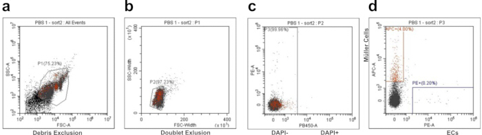
Figure 3: Flow cytometry gating strategy. Representative FACS gating strategy of a mouse intravitreally injected with PBS. (A) Debris exclusion. (B) doublet exclusion. (C) Cell viability stain using DAPI (DAPI-negative cells represent viable cells). (D) single positive GLAST1-APC cells (Müller Glia) and CD31-PE cells (endothelial cells [ECs]). Please click here to view a larger version of this figure.

To validate the pipeline, we performed single‑cell RNA sequencing on the sorted populations. As shown in Figure 4A, the major retinal cell types were successfully captured, and the targeted populations were markedly enriched compared to their native abundance, as reflected by the increased proportion of ECs and Müller glia relative to the viability filtered reference in Figure 3D. The cell-type annotations were supported by the expression of canonical marker genes across the identified populations (Figure 4A, Table 1). In particular, expression of Slc1a3 and Pecam1 localized to the corresponding Müller glia and EC populations, further supporting their identification (Figure 4C,D). Because ECs, photoreceptors, and other neural populations are known to exhibit relatively low transcriptional activity, we applied lower thresholds for the number of detected genes per cell during quality filtering to avoid excluding biologically relevant but transcriptionally quiescent cells.

To ensure that only high‑quality cells were retained for downstream analysis, we examined mitochondrial RNA content (Figure 4E). The majority of cells displayed mitochondrial RNA fractions well below 5%, indicating minimal dissociation‑induced cell death and confirming the overall high quality of the dataset.

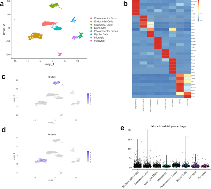
Figure 4: Retinal cell heterogeneity. (A) UMAP dimension reduction display of main retinal cell types, as well as relative enrichment of Endothelial Cells (orange) and Müller Glia (light green). (B) Heatmap, displaying canonical marker genes of major retinal cell populations. (C) UMAP dimension feature plot, showing the GLAST1 (Slc1a3) positive cell population. (D) UMAP dimension feature plot, showing the CD31 (Pecam1) positive cell population. (E) Scatter plot, displaying a low percentage of mitochondrial gene transcripts per each cell type. Please click here to view a larger version of this figure.

Cell Population	Number (Percentage)	Gene expression		UMI expression		Mitochondrial RNA expression
		Mean	Median	Mean	Median	Mean	Median
Photoreceptor rods	1342 (25.3%)	264.9	236	367.5	313	1.3%	1.0%
Endothelial cells	1404 (26.5%)	808.3	766.5	1687.7	1381	1.1%	0.7%
Müller glia	689 (13%)	608.6	574	1064	968	1.2%	1.0%
Monocytes	424 (8%)	529.2	494	1020.6	892	0.7%	0.6%
Photoreceptor cones	636 (12%)	500.7	472.5	756.7	679.5	1.3%	1.2%
Bipolar cells	313 (5.9%)	544.4	509	835.4	761	1.2%	0.9%
Microglia	274 (5.2%)	383.1	299.5	615.2	466	1.2%	0.9%
Pericytes	217 (4.1%)	959.9	926	2190.3	1943	0.9%	0.8%
Total	5299

Table 1: Quality metrics. Retinal cell detection, percentages, gene detection, unique molecular identifier (UMI) detection, mitochondrial RNA percentage.

Nevertheless, in the case of retinal samples, MHC1-based antibody hashing proved unreliable. As shown in Figure 5, hashing-based identification of the different treatment groups yielded reliable results for vascular endothelial cells, Müller cells/macroglia, microglia, monocytes/macrophages, and pericytes. Photoreceptors and bipolar cells, however, were not successfully labeled using MHC1 antibody hashing. Incomplete hashing reduced demultiplexing reliability when pooling multiple biological replicates/ multiple samples into a single 10x Genomics library preparation reaction. Therefore, carefully weigh the risks of losing sample identification vs the monetary benefits of pooling samples into one reaction.

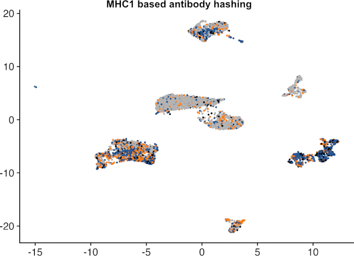
Figure 5: MHC1-based antibody hashing. Orange/blue representing positive hashing signals, grey coloring represents unhashed cells. Please click here to view a larger version of this figure.

Discussion

The present study describes a robust and reproducible workflow for the selective enrichment of retinal ECs and Müller glia from murine retina prior to single-cell RNA sequencing. Both cell populations are present at low abundance in the retina, making comprehensive characterization challenging with conventional unsorted single-cell approaches. By combining papain-based tissue dissociation with fluorescence-activated cell sorting using the established markers CD31 and GLAST1, we achieved reliable enrichment of both populations while retaining the overall cellular diversity of the retinal tissue. The resulting datasets contained the major retinal cell types and demonstrated a substantial increase in the representation of ECs and Müller glia compared to their physiological abundance (Table 1).

A central consideration for any single-cell transcriptomic workflow is the impact of tissue dissociation and cell sorting on cellular viability and transcriptional integrity.
While single-cell RNA sequencing provides high-resolution characterization of retinal cell populations, single-nucleus RNA sequencing is often favored for fragile tissues because of its reduced sensitivity to dissociation-induced stress and improved compatibility with archived samples¹². Retinal tissue is particularly susceptible to processing-induced perturbations because of its fragile neuronal architecture. Enzymatic dissociation and mechanical manipulation have been shown to activate stress-response pathways and alter the expression of immediate early genes¹³. Such effects cannot be completely avoided in the present workflow. However, all samples, including enriched fractions and unsorted retinal reference populations, were subjected to identical dissociation, staining, and sorting procedures. Moreover, single nuclei RNA sequencing does not allow for cell hashing or fluorescence-based cell sorting, as membrane-bound antigens are missing, therefore single-cell sequencing was favored in our approach.

To maintain cellular heterogeneity and avoid introducing selection bias during enrichment, an initial fraction of 50.000 DAPI-negative cells was collected prior to selective sorting, ensuring representation of the broader retinal cellular landscape. Consequently, potential dissociation-induced transcriptional changes are expected to affect all samples similarly, preserving the validity of relative comparisons between cell populations. The present workflow demonstrates that high-quality single-cell datasets can be generated from murine retina when tissue processing is carefully optimized.

The retina comprises a highly heterogeneous cellular environment that includes populations with markedly different transcriptional activity^14,15 and abundance¹⁶. Several retinal cell types exist in relatively quiescent states and naturally exhibit low RNA content, which can lead to their exclusion during standard quality-control filtering. Likewise, low abundant cell types that were not enriched might be missed due to their insignificant numbers. To avoid preferential loss of such populations, transcript count thresholds were intentionally lowered to at least 250 detected RNA transcripts per cell during downstream analysis. Despite these permissive filtering criteria, multiple quality metrics supported the integrity of the resulting datasets. Mitochondrial transcript fractions remained well below the commonly accepted 5% threshold associated with high-quality murine single-cell preparations¹⁷, and canonical marker gene expression enabled unambiguous identification of all cell clusters corresponding to the major retinal cell types. With the goal to focus on the inner blood retinal barrier, our protocol was designed to only enrich vascular endothelial cells and Müller cells. Low abundant amacrine cells, horizontal cells and retinal ganglion cells were not enriched and are not securely identified in the current dataset. Larger total cell numbers are needed to identify these rare populations. Retinal pigment epithelial cells are largely removed during retinal dissection and are therefore not expected to be detected in the resulting preparations. Adaption of the FACS protocol to enrich low abundant cell types is possible. Together, these findings indicate that the retained low-transcript cells largely reflect biological variation rather than technical artifacts, while rare cell types are only detected when large enough cell numbers are sequenced.

An additional methodological observation concerns sample multiplexing. MHC-I-based hashing strategies have been successfully applied in several murine tissues¹⁵; however, in our hands this approach did not provide reliable labeling of all retinal cells, likely owing to heterogeneous and often low MHC-I expression levels across some retinal cell populations¹⁸. Antibody-based sample assignment could not be performed with sufficient confidence for all cell types. This finding highlights the importance of validating multiplexing strategies in a tissue-specific manner before large-scale implementation.

A limitation of our enrichment strategy is its dependence on accessible cell-surface markers. Efficient fluorescence-activated cell sorting requires target populations to express suitable membrane-associated antigens that can be detected using fluorochrome-conjugated antibodies. CD31 and GLAST1 enabled robust enrichment of ECs and Müller glia/macroglia, respectively. In prior experiments, we confirmed that CD31+, CD45+ double-positive cells were not present in mouse tissue (data not shown). Moreover, we considered the expression of GLAST1 in astrocytes, however due to the diminishing relative percentage compared to GLAST positive Müller glia, we opted to not include further refining steps.

The adaptation of the workflow to other rare retinal populations will require the identification and validation of equally specific surface markers. Despite this requirement, the overall workflow is readily transferable and may facilitate the targeted investigation of additional low-abundance cell types in the retina and other heterogeneous tissues, especially as flow cytometry sorting allows selecting multiple different surface markers to securely identify relevant cell populations.

In conclusion, the presented workflow enables reliable enrichment of rare retinal ECs and Müller glia while preserving cellular diversity and transcriptomic quality. By combining optimized tissue dissociation, selective FACS enrichment, and quality-controlled single-cell RNA sequencing, the approach substantially increases the representation of low-abundance populations without compromising overall dataset integrity. This strategy provides a versatile framework for studying retinal cell biology, neurovascular interactions, and disease-associated cellular mechanisms at single-cell resolution.

Materials

List of materials used in this article

Name	Company	Catalog Number	Comments
1× DPBS	Gibco	14190169
5 mL Polystyrene Round-Bottom FACS Tube	Falcon	352058
Albumin Bovine Fraction V, Protease-Free (BSA)	SERVA	11926.03
Anti-Mo CD31 (PECAM-1)-PE	Invitrogen	12-0311-81
BD Pharmingen Purified Rat Anti-Mouse CD16/CD32 (Mouse BD Fc Block)	BD Bioscience	553142
Cell Tricks 30 µm Cell Strainer	Sysmex	04-0042-2316
Chromium i7 Multiplex Kit, 96 rxns	10x Genomics	PN-120262
Chromium Single Cell 3' Feature Barcode Library Kit, 16 rxns	10x Genomics	PN-1000079
Chromium Single Cell 3' GEM, Library and Gel Bead Kit v3, 4 rxns	10x Genomics	PN-1000092
Chromium Single Cell B Chip Kit, 16 rxns	10x Genomics	PN-1000074
Cytoflex SRT (FACS machine)	Beckman Coulter
DAPI	Invitrogen	62248
DNA Low Binding Tube 1.5 mL	Eppendorf	0030 108.051
EDTA 500 mM, pH 8.0	Invitrogen	AM9260G
Hanks’ Balanced Salt Solution (HBSS)	Gibco	14025092
HCl	Sigma-Aldrich	2,02,52,290
MACS BSA Stock Solution	Miltenyi Biotec	130-091-376
Papain Dissociation System (containing Papain, DNase, Ovomucoid)	Worthington Biochem.	LK003150
pH Meter	SI-Analytics	Lab 850
Rabbit anti-EAAT1/GLAST1/SLC1A3-APC	Biotechne	NB100-1869APC
TotalSeq-B0301 anti-mouse Hashtag 1-6	BioLegend	155831
R package	R	Version 4.5.1
Seurat	R	Version 5.4.0

References

- Peña JS, et al. Müller glia co-regulate barrier permeability with endothelial cells in an vitro model of hyperglycemia. Int J Mol Sci. 2024;25(22).
- Chavkin NW, Walsh K, Hirschi KK. Isolation of highly purified and viable retinal endothelial cells. J Vasc Res. 2021;58(1):49-57.
- Jeon C-J, Strettoi E, Masland RH. The major cell populations of the mouse retina. J Neurosci. 1998;18(21):8936.
- Chintalapudi SR, et al. Isolation and molecular profiling of primary mouse retinal ganglion cells: comparison of phenotypes from healthy and glaucomatous retinas. Front Aging Neurosci. 2016;8:93.
- Harada T, et al. Functions of the two glutamate transporters GLAST and GLT-1 in the retina. Proc Natl Acad Sci U S A. 1998;95(8):4663-6.
- Lertkiatmongkol P, et al. Endothelial functions of platelet/endothelial cell adhesion molecule-1 (CD31). Curr Opin Hematol. 2016;23(3):253-9.
- Stoeckius M, et al. Cell hashing with barcoded antibodies enables multiplexing and doublet detection for single cell genomics. Genome Biol. 2018;19(1):224.
- Attar M, et al. A practical solution for preserving single cells for RNA sequencing. Sci Rep. 2018;8(1):2151.
- du Halgouet A, et al. Multimodal profiling reveals site-specific adaptation and tissue residency hallmarks of γδ T cells across organs in mice. Nat Immunol. 2024;25(2):343-56.
- Team RC. R: A language and environment for statistical computing. R Foundation for Statistical Computing; Vienna, Austria; 2025.
- Hao Y, et al. Dictionary learning for integrative, multimodal and scalable single-cell analysis. Nat Biotechnol. 2024;42(2):293-304.
- Ding J, et al. Systematic comparison of single-cell and single-nucleus RNA-sequencing methods. Nat Biotechnol. 2020;38(6):737-46.
- Bondonese A, et al. Impact of enzymatic digestion on single cell suspension yield from peripheral human lung tissue. Cytometry A. 2023;103(10):777-85.
- Surzenko N, et al. SOX2 maintains the quiescent progenitor cell state of postnatal retinal Muller glia. Development. 2013;140(7):1445-56.
- Hamon A, et al. Linking YAP to Müller glia quiescence exit in the degenerative retina. Cell Rep. 2019;27(6):1712-25.e6.
- Fadl BR, et al. An optimized protocol for retina single-cell RNA sequencing. Mol Vis. 2020;26:705-17.
- Osorio D, Cai JJ. Systematic determination of the mitochondrial proportion in human and mice tissues for single-cell RNA-sequencing data quality control. Bioinformatics. 2021;37(7):963-7.
- Liu J, et al. The expression pattern of classical MHC class I molecules in the development of mouse central nervous system. Neurochem Res. 2013;38(2):290-9.
Reprints and Permissions
This article has been published
Video Coming Soon