Predicting Oxaliplatin-Induced Severe Neuropathy in Colorectal Cancer Patients with Diabetic Polyneuropathy

Summary

This study develops an interpretable machine learning approach using XGBoost and SHAP analysis to predict oxaliplatin-induced dose-limiting neurotoxicity in colorectal cancer patients with diabetic peripheral neuropathy and to characterize model-level associations among clinical risk factors.

Abstract

Colorectal cancer (CRC) patients with comorbid diabetic peripheral neuropathy (DPN) face an increased risk of oxaliplatin-induced dose-limiting toxicity (DLT). This study aimed to develop a machine learning model to predict chemotherapy tolerance and investigate nonlinear feature associations within the predictive framework. We retrospectively analyzed 513 CRC patients with DPN. Five machine learning algorithms were developed and evaluated, and SHapley Additive exPlanations (SHAP) were used to explore feature associations. The XGBoost model demonstrated the highest discriminative performance in predicting DLT (AUC = 0.880), significantly outperforming logistic regression (p = 0.002). SHAP analysis showed that cumulative oxaliplatin dose, poor glycemic control (HbA1c > 8.0%), and systemic inflammation (NLR) were associated with increased model-predicted risk of DLT. Interaction analyses further identified nonlinear model-level associations between oxaliplatin exposure and metabolic and neurological features. The XGBoost model combined with SHAP explanations provides an exploratory framework for dynamic risk stratification during treatment. These findings represent associative predictive patterns and require prospective, external validation before clinical application.

Introduction

Oxaliplatin-based chemotherapy remains a standard treatment modality for patients with colorectal cancer (CRC)^1,2. However, its clinical use is often impaired by peripheral neuropathy induced by oxaliplatin, which commonly occurs as a dose-limiting toxicity (DLT)³. This is a specific clinical dilemma in CRC patients with comorbid diabetic peripheral neuropathy (DPN)⁴. Neuronal vulnerability to platinum-based agents might depend on preexisting nerve damage and chronic metabolic dysregulation⁵. Furthermore, the resulting superimposed neurotoxicity is often irreversible, potentially leading to persistent sensory and motor dysfunction that significantly diminishes the patients' long-term quality of life⁶. As a result, the given comorbid group is at an increased risk of experiencing premature treatment interruption, which can have a negative impact on long-term oncology prognosis⁷.

Although this comorbidity has clinical importance, there is limited accuracy in the risk prediction of chemotherapy tolerance in this subpopulation⁸. The existing prognostic and risk assessment models are mainly based on conventional linear statistical models and anatomical tumor, node, metastasis (TNM) stages⁹. These traditional methods might not be adequate to measure the complex, nonlinear relationship between cumulative pharmacological exposure, systemic inflammation, and metabolic indices like glycated hemoglobin (HbA1c)¹⁰. Consequently, clinicians do not necessarily have accurate, personalized evaluation tools that can be used proactively to identify the patients who are at the greatest risk of developing severe, irreversible neurotoxicity dynamically during the course of treatment, accounting for planned cumulative exposures¹¹.

Machine learning algorithms have become a tool for analyzing complex clinical data and may improve predictive performance over traditional statistics by detecting high-dimensional patterns¹². In order to overcome the inherent black-box nature of more advanced predictive algorithms, interpretable models like SHapley Additive exPlanations (SHAP) may be employed to visualize feature impacts and their underlying relationships¹³. Thus, the main aim of this investigation was to design and contrast various machine learning models to predict DLT among CRC patients with comorbid DPN. Moreover, we aimed to use SHAP analysis to clarify the nonlinear relationships and potential synergies among clinical risk factors, ultimately providing a methodological guide for individualized risk stratification and clinical management.

Protocol

This retrospective observational study was conducted utilizing clinical data collected between January, 2020 and December, 2025. The study protocol was reviewed and approved by the Institutional Review Board of Second People's Hospital of Yibin (Approval Number: 2026-029). All procedures were conducted in accordance with the principles outlined in the Declaration of Helsinki. Given the retrospective nature of the study, the requirement for written informed consent was waived.

Patient selection criteria

The study population comprised patients who met the following inclusion criteria: (1) pathologically diagnosed with colorectal cancer; (2) documented clinical history of type 2 diabetes mellitus complicated by diabetic peripheral neuropathy prior to chemotherapy; (3) received oxaliplatin-based chemotherapy regimens; and (4) availability of complete baseline clinical and neurophysiological data. Patients were excluded if they: (1) presented with preexisting peripheral neuropathy attributed to other etiologies, such as alcohol abuse, severe nutritional deficiency, or previous exposure to other neurotoxic agents; (2) had severe concurrent malignancies, severe renal or hepatic dysfunction before treatment; or (3) lacked essential follow-up records for toxicity evaluation.

Clinical variables and outcome definition

A total of 15 clinical features, encompassing both baseline and treatment-related variables, were extracted from the electronic medical records. Demographic and anthropometric variables included Age (years), Body Mass Index (BMI, kg/m² ), and Skeletal Muscle Index (SMI, cm²/m²). Metabolic and neurological features consisted of Glycated Hemoglobin (HbA1c, %), Fasting Blood Glucose (FBG, mmol/L), Duration of Diabetes (years), baseline Toronto Clinical Neuropathy Score (TCNS, points), Sural Nerve Conduction Velocity (NCV, m/s), and Serum Vitamin B12 (pg/mL). Oncological and treatment-related characteristics included Tumor TNM Stage, Cumulative Oxaliplatin dose (mg/m²), and Carcinoembryonic Antigen (CEA, ng/mL). Systemic and inflammatory indicators comprised the Neutrophil-to-Lymphocyte Ratio (NLR), estimated Glomerular Filtration Rate (eGFR, mL/min/1.73 m²), and Serum Albumin (g/L). The primary endpoint was the occurrence of dose-limiting toxicity (DLT), defined as the delay, dose reduction, or early discontinuation of oxaliplatin primarily due to severe peripheral neurotoxicity. To minimize retrospective ascertainment bias, the DLT endpoint was adjudicated via electronic medical record review by two independent clinical oncologists. Cases where treatment modifications were clearly attributed to disease progression, severe hematological toxicities, or gastrointestinal toxicities, rather than neurotoxicity, were strictly excluded from the DLT cohort.

Secondary clinical outcomes evaluation

To support the clinical translation analysis, chemotherapy-induced peripheral neuropathy (CIPN) severity was retrospectively graded from medical records using the National Cancer Institute Common Terminology Criteria for Adverse Events (NCI-CTCAE) version 5.0. Patient-reported symptom burden and quality of life (QoL) outcomes were derived from the European Organisation for Research and Treatment of Cancer Quality of Life Questionnaire CIPN twenty-item scale (EORTC QLQ-CIPN20), which focuses on sensory, motor, and autonomic domains, evaluated at the end of the scheduled chemotherapy regimen.

Machine learning algorithms and hyperparameter configuration

Five machine learning algorithms, eXtreme Gradient Boosting (XGBoost), Random Forest (RF), Support Vector Machine (SVM), k-Nearest Neighbors (KNN), and Logistic Regression (LR), were created to assess chemotherapy tolerance. Prior to model development, variables with more than 10% missing values were excluded. For the remaining variables, missing data were handled using median imputation. Importantly, to prevent data leakage, imputation and feature scaling (standardization for continuous variables in SVM and KNN models) were performed strictly after the dataset partition, utilizing parameters derived solely from the training set. A fixed random seed (set.seed(202405)) was employed to partition the dataset into a training cohort (75%) and an internal hold-out testing cohort (25%). A systematic grid search, coupled with 5-fold cross-validation on the training set, was used to optimize hyperparameters. For the final XGBoost model, the selected hyperparameters included a maximum tree depth (max_depth) of 4, a learning rate (eta) of 0.05, and 100 boosting rounds (nrounds). The RF model utilized 300 decision trees (ntree = 300). The SVM model employed a radial basis function kernel, and the KNN algorithm was configured with 7 nearest neighbors (k = 7). The optimal decision threshold for binary classification in the confusion matrix was determined using Youden's Index derived from the ROC curve on the training set.

Regarding the distribution of classes, the examined cohort presented a relatively balanced proportion of the non-DLT (n = 272) and DLT (n = 241) groups. To address residual bias and ensure a robust evaluation, performance measures less sensitive to class distribution, e.g., the Area Under the Precision-Recall Curve (AUC-PR) and the Brier score, were prioritized alongside the conventional Receiver Operating Characteristic (ROC) analysis.

Statistical and interpretability analysis

Continuous variables were summarized as means and standard deviations (SD) or medians and interquartile ranges (IQR), and compared via either Student’s t-test or Mann–Whitney U (MWU) test depending on data distribution. Categorical variables were presented as frequencies and percentages, and compared using the Chi-square test. To quantify the magnitude of differences between the tolerance groups beyond statistical significance, effect sizes were calculated as the Standardized Mean Difference (SMD) for all baseline variables. The DeLong test was implemented for comparing AUC values of the models. SHapley Additive exPlanations (SHAP) were used for extracting feature importance, interaction matrices, and individual, localized SHAP values. All statistical computing and Machine Learning analyses were performed using R Software (version 4.3.1). A two-sided p-value of 0.05 was valued as significant.

Results

=Baseline characteristics and comorbidity landscape

A total of 513 colorectal cancer patients with comorbid diabetic peripheral neuropathy were included in this study, comprising 241 patients who experienced dose-limiting toxicity (DLT group) and 272 who did not (Non-DLT group). Table 1 summarizes the baseline clinical and demographic features. The tumor TNM stage did not differ significantly between the two groups (p = 0.468), indicating that the incidence of DLT was not more likely attributable to an advanced oncological stage and may be more directly associated with host factors and comorbidity status. Patients in the DLT group had an elevated baseline Toronto Clinical Neuropathy Score (TCNS), a reduced skeletal muscle index (SMI), worse glycemic control (higher HbA1c and fasting blood glucose), and increased systemic inflammation (NLR) compared with the Non-DLT group (all p < 0.05).

Interestingly, the cumulative oxaliplatin dose was greater in the DLT group than in the Non-DLT group (605.44 vs. 543.71 mg/m², p < 0.001). As shown in the density distribution in Figure 1A, the exposure of oxaliplatin in the DLT cohort shifted towards a higher dosage range. This finding can be indicative of the dose-cumulative nature of the oxaliplatin induced neuropathy. A higher chance of reaching the neurotoxic threshold occurs in patients who have a longer planned schedule of therapy, and lower chances of patients developing severe toxicity occur in patients who are on short-course therapies. Moreover, Figure 1E shows that the sural nerve conduction velocity (NCV) before chemotherapy was notably lower in the DLT group, suggesting nerve impairment as a risk factor.

In order to create a graphical representation of the comorbidity, a Venn diagram was created (Figure 1B), which reveals that there is significant overlap between three key risk factors, namely high dose of oxaliplatin, inadequately controlled glycemic levels, and abnormal NCV, with 214 patients exhibiting all these characteristics. Spearman correlation analysis (Figure 1C) showed anticipated physiological correlations between metabolic, inflammatory, and neurological indices. Though there was a positive correlation between HbA1c and baseline TCNS (Figure 1D), the correlation coefficient was low (R = 0.17, p < 0.001). This dispersion suggests that linear associations with individual variables may not be sufficient to capture the severity of neuropathy in this group. Likewise, Principal Component Analysis (PCA) revealed significant overlap of the DLT versus Non-DLT groups on the first two principal components (Figure 1F). The fact that traditional linear dimensionality reduction cannot effectively disentangle the cohorts suggests nonlinear interactions among these clinical characteristics, thereby justifying the use of machine learning algorithms in subsequent analyses.

Development and performance evaluation of machine learning models

Given the complex, nonlinear interactions suggested by the baseline clustering analysis, five machine learning models were developed and evaluated in an internal hold-out testing cohort (N = 128). Figure 2A presents the Receiver Operating Characteristic (ROC) curves, which show that the XGBoost model performed best based on a better Area Under the Curve (AUC = 0.880; 95% CI, 0.815-0.945), in comparison to a more traditional logistic regression (LR) model (AUC = 0.783; 95% CI, 0.698-0.868). A DeLong test revealed a statistically significant difference between XGBoost and LR (p = 0.002), suggesting that tree-based algorithms can capture more complex interactions underlying toxicity-driven comorbidity patterns. This benefit persisted after PR analysis (Figure 2C), with XGBoost consistently achieving the highest AUC-PR (0.870).

To convert the predicted probabilities into a clinical classification, a confusion matrix of the XGBoost model was plotted (Figure 2B). In the independent testing cohort (N = 128), there were 45 patients who actually experienced dose-limiting toxicity (DLT) and 83 patients who did not. The model accurately identified 39 true positives and 65 true negatives, yielding a sensitivity of 86.67% (39/45) and a specificity of 78.31% (65/83), accompanied by 6 false negatives and 18 false positives. This relatively high sensitivity of such a predictive assay is likely to be extremely valuable in an oncology practice, where missing out on a patient at risk for severe neurotoxicity could result in potentially irreversible nerve damage.

Second, to minimize the bias of small sample variance from the limited testing cohort, a calibration curve was constructed (Figure 2D) using a quintile binning method. Predicted probabilities closely followed the diagonal reference line, and the observed event fractions indicated satisfactory calibration in this model's risk estimation. Pairwise comparison of clinical utility by Decision Curve Analysis (DCA) was performed (Figure 2E). The net benefit of the XGBoost model was greater across a range of clinically relevant threshold probabilities (approximately 0.10 to 0.60) than that of the LR model, as well as for treat-all or treat-none strategies. The small fluctuations at very high thresholds (i.e., above 0.75) are probably just mathematical artifacts that arise from the limited number of positive predictions in this part of the testing set.

Lastly, overall errors of the models were quantified (Figure 2F). XGBoost also had the lowest Brier Score (0.140) and Log-Loss (0.435) out of all algorithms assessed, consistent with its discriminative performance, followed by Random Forest (Brier Score = 0.168, Log-Loss = 0.507). Upon performing these comprehensive evaluations, the XGBoost model was chosen as the best in class algorithm for the subsequent interpretability analysis.

Global interpretability and nonlinear feature associations via SHAP analysis

To understand the mechanisms driving the XGBoost model's predictions, SHapley Additive exPlanations (SHAP) were employed to evaluate global feature importance and potential interactions. The SHAP summary plot (Figure 3A) and the bar chart of mean absolute SHAP values (Figure 3B) identify cumulative oxaliplatin dose (mean |SHAP| = 0.461) and sural nerve NCV (mean |SHAP| = 0.412) as the features of greatest importance to the model output, supporting the critical role of drug exposure and nerve integrity at baseline in the model of chemotherapy tolerance. Among the blood and systemic functions, NLR (0.342) and SMI (0.320) ranked higher than HbA1c (0.121) and baseline TCNS (0.137). It appears that, even though glycemic control and the pre-existence of diabetes and neuropathy are highly relevant, the systemic and generalized impact may dominate across the study cohort.

In addition to the importance of individual features, the SHAP interaction matrix (Figure 3C) illustrates multiple, synergistic relationships among clinical parameters. The cumulative oxaliplatin dose interacted synergistically with numerous other factors, suggesting that dose-limiting toxicity (DLT) may result from the combined impact of oxaliplatin exposure and additional clinical comorbidities.

To better understand these nonlinear relationships, SHAP dependence plots were created. The dependence plot of HbA1c (Figure 3D) showed a clear nonlinear relationship, with SHAP values (i.e., risk) increasing sharply once HbA1c levels exceeded 8.0%. The coloring of the points indicated that risk values increased among the few patients with severe poor glycemic control and high oxaliplatin levels, pointing towards a possible metabolic-pharmacological synergy. In addition, Figure 3E showed that the relationship between oxaliplatin and risk was modest until a cumulative threshold was reached, at which point risk sharply increased, particularly in patients with poor glycemic control (high HbA1c levels). Furthermore, Figure 3F showed the relationship between baseline TCNS and systemic inflammation (NLR). The plot shows that the risk of DLT further increases in patients with greater baseline neuropathy and higher inflammation (NLR), as indicated by red points. Therefore, the results showed that poor glycemic control and systemic inflammation demonstrated a strong nonlinear association with an amplified predicted risk of oxaliplatin-related neurotoxicity within the model's feature space.

Individualized precision medicine profiling via local SHAP explanations

While global SHAP analysis revealed population-level trends, local SHAP explanations were utilized to evaluate how the model might assist in individualized clinical decision-making. To demonstrate the localization of risk factor accumulation and interaction, we have selected three representative patient profiles and visualized them using SHAP waterfall and force plots (Figure 4).

Figure 4A and Figure 4B show a high-risk patient who experienced a dose-limiting toxicity (DLT), with a predicted risk of 92.5%. The waterfall plot is a quantitative measure of the process of accumulating risk from the baseline expected log-odds (E[f(x)] = -0.121) up to the ultimate prediction (f(x) = 2.52). Interestingly, in combination with a rather high cumulative dose of oxaliplatin (675 mg/m2), poor glycemic control (HbA1c = 9.6%) and impaired baseline renal function (eGFR = 79.4 mL/min/1.73m2) yielded large positive SHAP values (indicated by red bars/arrows). The accompanying force diagram (Figure 4B) illustrates that these variables combined to yield a substantial positive shift in the model's output, outweighing the protective contributions of the features and pushing the final prediction into a high-risk zone of severe neurotoxicity.

On the other hand, Figure 4C,D represent a low-risk patient (predicted risk: 4.7%) who was able to complete chemotherapy without any DLT. In this case, good baseline nerve functioning (sural nerve NCV = 46.4 m/s and TCNS = 3 points) and moderate exposure to oxaliplatin (495 mg/m²) contributed to large negative SHAP values (blue bars/arrows). As shown in the force plot (Figure 4D), these protective features effectively counteracted the treatment's inherent mild toxicity, keeping the final prediction well below the safety threshold.

The potential clinical utility of machine learning is especially emphasized in borderline cases, as illustrated by Patient C (Figure 4E,F), with a predicted risk probability of 50.4%. The force plot shows a clearly competing set of opposing forces where a severely impaired baseline nerve conduction (sural nerve NCV = 26.3 m/s) has a strong positive impact towards toxicity (red) that was almost countered by protective measures like adequate skeletal muscle index (SMI = 44.7 cm²/m²) and optimal glycemic control (HbA1c = 7.0%). These visualizations indicate that the optimality of metabolic and nutritional status in such patients with preexisting neuropathic damage may serve as an important buffer. These personalized profiles illustrate how individual clinical features contribute to model-predicted risk; however, their utility for guiding clinical interventions requires prospective validation.

Clinical translation and risk stratification based on the AI model

To evaluate the translational potential of the proposed AI model in real-world clinical settings, the continuous predicted probabilities generated by XGBoost were utilized to stratify the patient cohort into three distinct risk groups: Low Risk (probability < 0.30), Intermediate Risk (0.30 - 0.70), and High Risk (> 0.70). These exploratory thresholds were determined based on the approximate tertile distribution of predicted probabilities derived from the training set, rather than being pre-specified clinical cutoffs. Risk stratification (Figure 5A) showed a substantial separation in clinical outcomes, with real DLT (red dots) events clustering within the High Risk zone, supporting the model’s population-level discrimination.

The Sankey diagram (Figure 5B) further illustrated the AI-derived stratification, showing the patient pathway through the TNM framework and AI risk strata, as well as clinical outcomes. The alluvial plot indicated that, despite belonging to the same conventional oncology stage (Stage II or Stage III), the patients in the AI model were shifted to different risk pathways. High-risk patients, regardless of their traditional stage, consistently flowed toward the DLT outcome, suggesting that the AI model may surpass traditional staging models by accounting for patient prognostics and comorbidities.

Risk strata post-chemotherapy were directly associated with clinical severity. As shown in the stacked bar chart (Figure 5C), the likelihood of developing Grade 3+ CIPN (potentially irreversible) increased with their grouping (Chi-square p < 0.001). Grade 3+ CIPN was reported in only 3.6% of the Low Risk group and 64.2% of the High Risk group. Lastly, patient-reported symptom burden beyond grade was quantified and shown across QoL domains, with High Risk patients exhibiting a larger polygon area (indicating greater symptom burden) across multiple facets of impairment compared to Low Risk patients (Figure 5D).

A risk trajectory curve was plotted (Figure 5E) to illustrate the existence of more complex nonlinear clinical dynamics. Across baseline TCNS scores, a higher DLT risk was predicted for patients with poor glycemic control (HbA1c > 8.0%) versus patients with good control. Overall, this observation aligns with the hypothesis that optimal glycemic control may not eliminate the neurotoxic risk associated with baseline nerve damage, but may decrease risk. The gap in the full-course chemotherapy completion rates among the different risk strata is illustrated in Figure 5F. The Low Risk group completion rate was 87.1% (SE = 2.4%), while the rate for the High Risk group was only 10.9% (SE = 2.4%, p < 0.001). Based on these observations, the AI-derived risk stratification approach shows potential in characterizing patient vulnerability to treatment. However, given the lack of external validation in the current study, this framework is purely exploratory. It provides a methodological reference for future research but is not yet ready for direct clinical application to guide dose adjustments or mitigation efforts.

DATA AVAILABILITY:

To promote research reproducibility, the fully de-identified underlying clinical dataset and the custom R code used for machine learning analyses and visualizations in this study are provided as Supplementary Materials (Supplementary File 1 and Supplementary Coding File 1, respectively) available with this article.

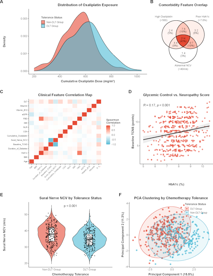
Figure 1: Baseline comorbidity landscape and clinical feature distributions of the study cohort. (A) Density plot showing the distribution of cumulative oxaliplatin dose between the DLT and non-DLT groups. (B) Venn diagram illustrating the overlap of three comorbidity features: high oxaliplatin dose, poor HbA1c, and abnormal NCV. (C) Heatmap presenting the Spearman correlation among clinical variables. (D) Scatter plot indicating a potential positive association between HbA1c levels and baseline TCNS points. (E) Violin plot comparing the sural nerve NCV between different chemotherapy tolerance statuses. (F) Principal Component Analysis (PCA) plot showing the overall clustering tendency of the cohort based on tolerance status. Please click here to view a larger version of this figure.

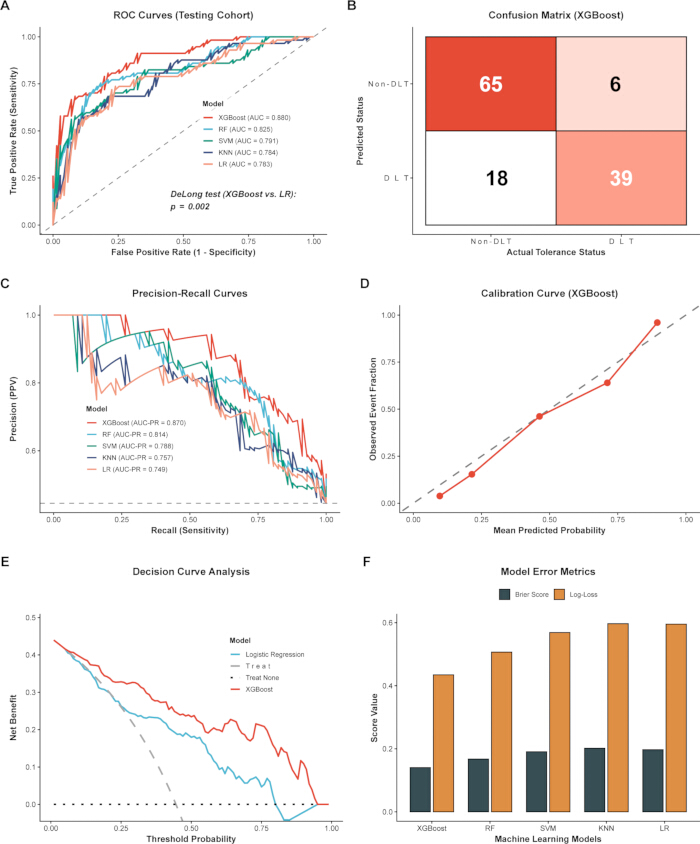
Figure 2: Performance evaluation of the machine learning models in the testing cohort. (A) Receiver Operating Characteristic (ROC) curves of the five machine learning algorithms. The DeLong test was used to compare the AUC between XGBoost and Logistic Regression (LR). (B) Confusion matrix illustrating the classification results of the XGBoost model. (C) Precision-Recall (PR) curves for the evaluated models. (D) Calibration curve indicating the agreement between XGBoost-predicted probabilities and observed event fractions. (E) Decision Curve Analysis (DCA) suggesting the potential net clinical benefit of the models across different threshold probabilities. (F) Bar chart presenting the model error metrics, including Brier Score and Log-Loss. Please click here to view a larger version of this figure.

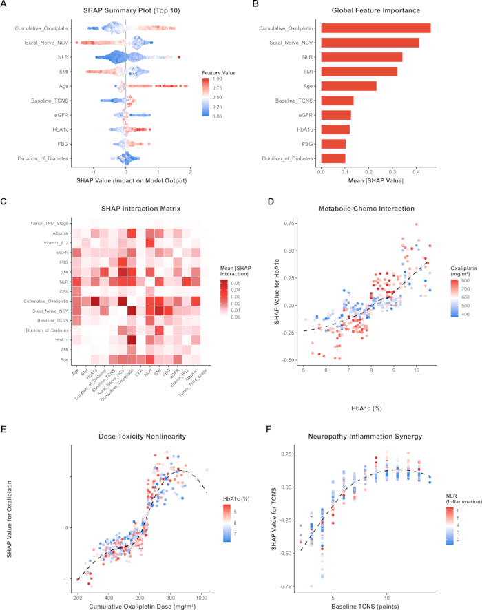
Figure 3: Global SHAP (SHapley Additive exPlanations) analysis for the XGBoost model. (A) SHAP summary plot indicating the distribution of SHAP values for the top 10 features, where color represents the feature value. (B) Bar chart showing the global feature importance ranked by mean absolute SHAP values. (C) SHAP interaction matrix presenting the mean absolute interaction values among variables. (D–F) SHAP dependence plots illustrating the nonlinear trajectories and potential interaction effects of specific features: (D) HbA1c colored by cumulative oxaliplatin dose, (E) cumulative oxaliplatin dose colored by HbA1c, and (F) baseline TCNS colored by the neutrophil-to-lymphocyte ratio (NLR). Please click here to view a larger version of this figure.

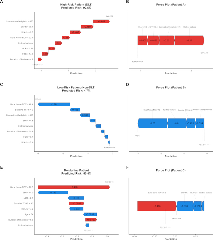
Figure 4: Individualized patient profiling using local SHAP explanations. SHAP waterfall and force plots are presented for three representative clinical cases to illustrate how individual features may drive the model's predictions: (A, B) a high-risk patient who experienced DLT; (C,D) a low-risk patient without DLT; and (E,F) a borderline patient. Red bars/arrows indicate features that increase the predicted risk of DLT, while blue bars/arrows indicate features that decrease the risk. Please click here to view a larger version of this figure.

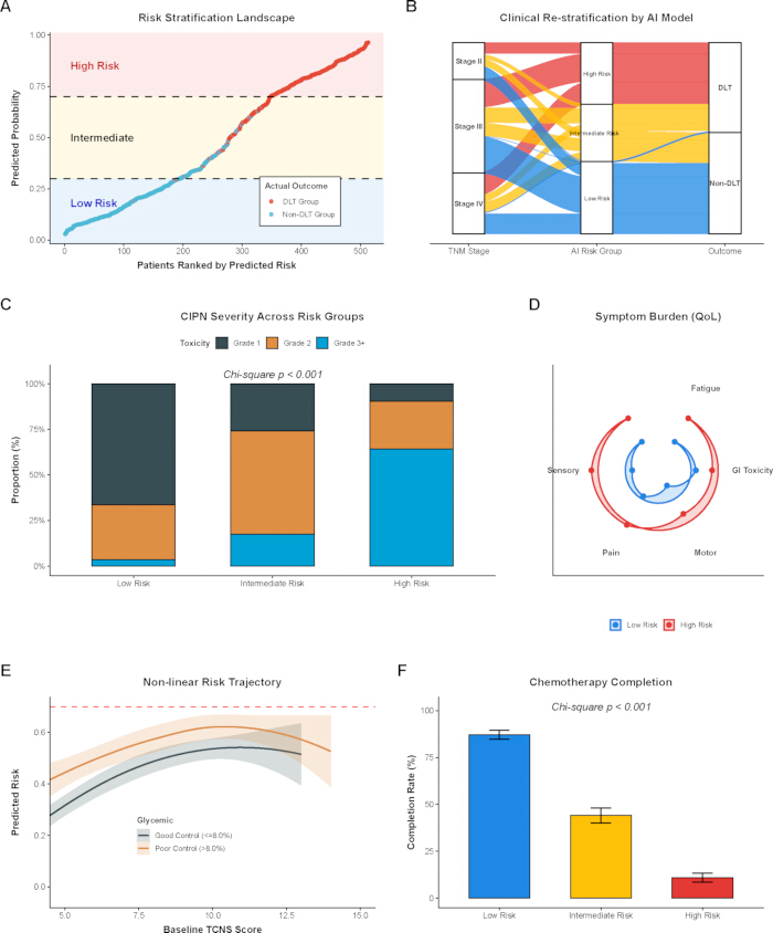
Figure 5: Clinical risk stratification and its association with therapeutic outcomes. (A) Risk stratification landscape sorting patients by AI-predicted probability into low, intermediate, and high-risk groups. (B) Sankey diagram illustrating the patient flow from traditional TNM stages to AI-assigned risk groups, and subsequently to the clinical outcomes. (C) Stacked bar chart showing the distribution of CIPN severity across different risk groups. (D) Radar chart indicating the average symptom burden (quality of life dimensions) for the low- and high-risk groups. (E) Nonlinear risk trajectory suggesting the relationship between baseline TCNS and predicted risk, stratified by glycemic control status. (F) Bar chart presenting the full-course chemotherapy completion rates among the three risk groups. Please click here to view a larger version of this figure.

Clinical Characteristics	Total Cohort (N=513)	Non-DLT Group (N=272)	DLT Group (N=241)	Effect Size (SMD)	P-value
Demographic and Anthropometric
Age (years), mean (SD)	62.00 (8.67)	60.66 (8.13)	63.51 (9.02)	0.332	<0.001
BMI (kg/m²), mean (SD)	24.27 (3.59)	24.11 (3.50)	24.44 (3.68)	0.092	0.305
SMI (cm²/m²), mean (SD)	42.54 (6.17)	43.64 (6.27)	41.30 (5.81)	0.387	<0.001
Metabolic and Neurological
HbA1c (%), median [IQR]	8.00 [7.30, 8.70]	7.80 [7.20, 8.60]	8.20 [7.40, 8.90]	0.384	0.001
Fasting Blood Glucose (mmol/L), mean (SD)	8.80 (1.52)	8.63 (1.45)	9.00 (1.58)	0.245	0.006
Duration of Diabetes (years), median [IQR]	7.60 [4.90, 11.40]	7.40 [4.70, 11.60]	8.00 [5.20, 11.00]	0.082	0.459
Baseline TCNS (points), median [IQR]	8.00 [5.00, 10.00]	7.00 [4.00, 10.00]	9.00 [7.00, 11.00]	0.65	<0.001
Sural Nerve NCV (m/s), mean (SD)	36.25 (5.41)	37.58 (5.60)	34.74 (4.76)	0.546	<0.001
Serum Vitamin B12 (pg/mL), median [IQR]	457.00 [368.00, 525.00]	448.50 [367.25, 525.00]	464.00 [368.00, 524.00]	0.075	0.52
Oncological and Treatment-Related
Tumor TNM Stage, n (%)				0.088	0.468
Stage II	99 (19.3)	57 (21.0)	42 (17.4)
Stage III	251 (48.9)	134 (49.3)	117 (48.5)
Stage IV	163 (31.8)	81 (29.8)	82 (34.0)
Cumulative Oxaliplatin (mg/m²), mean (SD)	572.71 (136.05)	543.71 (127.63)	605.44 (138.07)	0.464	<0.001
CEA (ng/mL), median [IQR]	12.50 [6.50, 21.30]	12.30 [6.47, 20.85]	12.50 [6.90, 22.70]	0.041	0.703
Systemic and Inflammatory
NLR, median [IQR]	2.74 [1.98, 3.99]	2.44 [1.85, 3.55]	3.11 [2.21, 4.31]	0.42	<0.001
eGFR (mL/min/1.73m²), mean (SD)	94.97 (12.60)	96.17 (12.38)	93.62 (12.72)	0.203	0.022
Serum Albumin (g/L), mean (SD)	38.20 (4.65)	38.22 (4.72)	38.17 (4.58)	0.011	0.915

Table 1: Baseline characteristics of colorectal cancer patients with comorbid diabetic peripheral neuropathy, stratified by chemotherapy tolerance. Note: Data are presented as mean (standard deviation, SD) for normally distributed continuous variables, median [interquartile range, IQR] for skewed continuous variables, and number (%) for categorical variables. Statistical differences were evaluated using Student's t-test, Mann-Whitney U test, or Chi-square test, as appropriate. Effect sizes are reported as the Standardized Mean Difference (SMD), where an SMD value > 0.10 indicates a meaningful imbalance between the groups.
Abbreviations: DLT, Dose-Limiting Toxicity; BMI, Body Mass Index; SMI, Skeletal Muscle Index; HbA1c, Glycated Hemoglobin; TCNS, Toronto Clinical Neuropathy Score; NCV, Nerve Conduction Velocity; TNM, Tumor, Node, Metastasis; CEA, Carcinoembryonic Antigen; NLR, Neutrophil-to-Lymphocyte Ratio; eGFR, estimated Glomerular Filtration Rate.

Supplementary File 1: De-identified clinical dataset. Please click here to download this file.

Supplementary Coding File 1: Custom R code used for machine learning analyses and visualizations in this study. Please click here to download this file.

Discussion

Colorectal cancer patients with comorbid diabetic peripheral neuropathy frequently face severe neurotoxicity during oxaliplatin-based chemotherapy, presenting a significant challenge in clinical oncology¹⁴. This study developed an XGBoost machine learning model and applied SHAP analysis, suggesting that synergistic interactions among cumulative oxaliplatin dose, glycemic control, and systemic frailty are strongly correlated with chemotherapy tolerance and the occurrence of dose-limiting toxicity.

The XGBoost algorithm achieved better results than conventional logistic regression. This conclusion is consistent with prior research indicating that tree-based models tend to perform better on high-dimensional clinical data¹⁵. A widely discussed issue in oncology is whether traditional anatomical staging is adequate for assessing toxicity risk¹⁶. The AI model effectively restratifies patients with the same TNM staging into distinct pathways based on toxicity risk, as shown in the Sankey diagram (Figure 5B). This model suggests that anatomical staging alone may be an inadequate predictor of pharmacologic tolerance. Additionally, the baseline data showed an atypical trend: patients in the DLT group received more oxaliplatin. This could be explained by the cumulative dose-dependent nature of oxaliplatin neuropathy: patients on long-term regimens are more prone to surpass the neurotoxic threshold, whereas patients on short adjuvant regimens manage to complete their treatment before severe toxicity occurs^17,18.

The global SHAP analysis informed the model on how features are connected. While traditional oncology prioritizes cumulative dose as the dominant factor in drug-induced neuropathy, the interaction matrix (Figure 3) suggests a possible synergy between oxaliplatin exposure and the patient's baseline HbA1c levels. A high HbA1c value indicates worse glycemic control, and glycemic variability may be a chronic factor in damaging the blood-nerve barrier¹⁹. Schwann cells may become more susceptible to damage from platinum-based drugs²⁰. It is crucial to emphasize that SHAP analysis strictly quantifies mathematical feature contributions and associative interactions within the predictive boundaries of the XGBoost model. Although these nonlinear model-level interactions (such as those observed among oxaliplatin dose, HbA1c, and inflammation) align with certain clinical hypotheses, they cannot, in principle, establish true biological causality or prove direct physiological synergy²¹. These computational findings should be interpreted solely as associative risk patterns warranting future biological validation. At the same time, systemic indicators such as the neutrophil-to-lymphocyte ratio and skeletal muscle index ranked higher in overall feature importance than specific markers like HbA1c. This means systemic inflammation and sarcopenia are hypothesized to reduce treatment tolerance across the entire cohort, compared with specific metabolic markers such as HbA1c. SHAP values indicate that traditional linear analyses may fail to detect these critical nonlinear catalytic dynamics.

The potential individual- and population-level clinical tools were illustrated through contextual risk stratifications and local SHAP explanations. For borderline patients, the force plots (Figure 4) capture the balance between protective and deleterious forces. The risk stratifications, along with the SHAP, dynamically matched the actual clinical outcomes. Mild neuropathy incidence and the full course of chemotherapy completion were other clinical outcomes considered. The minor fluctuations observed at the extreme-high thresholds of the decision curves are likely mathematical artifacts due to the limited absolute number of high-risk patients, rather than inherent model instability²². However, it should be noted that the risk-stratification thresholds (0.30 and 0.70) were exploratory and derived from the training data distribution. Consequently, evaluating secondary outcomes (e.g., severe CIPN and completion rates) based on these post hoc, model-derived strata carries an inherent risk of circular inference, necessitating future validation using pre-specified clinical cutoffs.

This study also has several limitations. First and foremost, it is a single-center retrospective study that relies exclusively on a random-split internal validation. No independent external dataset was utilized to evaluate the model's performance. Consequently, the real-world generalizability of the XGBoost model remains unproven, as the findings may be inherently biased toward the specific demographic characteristics and localized clinical management protocols of our institution. Secondly, a major study limitation was that the model did not incorporate certain crucial unmeasured confounding variables. Most notably, pharmacogenomic data, such as specific genetic polymorphisms related to platinum-induced peripheral neuropathy (e.g., variants in DNA repair, transport, or drug metabolism pathways), were not collected. This important source of inter-patient biological variability remains unaccounted for in our current predictive architecture and represents a notable constraint of the present clinical dataset. Because of these unaddressed inter-patient variances and the lack of external validation, we must emphasize that the model presented herein is purely exploratory. It is not ready for direct clinical application. Future multicenter, prospective validation is strictly required before considering any clinical translation. Thirdly, the inclusion of cumulative oxaliplatin dose as a feature means this model functions as a dynamic risk simulator during therapy rather than a strictly baseline, pre-treatment prediction tool. The inherent correlation between cumulative dose and treatment duration necessitates careful interpretation when applying these findings to pre-treatment decision-making.

Conclusion

This research constructed an XGBoost-powered prediction model specialized in chemotherapy tolerance for colorectal cancer patients suffering from diabetic peripheral neuropathy. The model demonstrated initial computational feasibility in stratifying toxicity risk for this specific comorbid population within the internal cohort. SHAP analysis showed model-level associations and potential interactions between oxaliplatin exposure, glycemic control, systemic markers, and predicted dose-limiting neurotoxicity. Implementing local SHAP risk stratification helped predict certain aspects of the clinical context in this study. Visualizations derived from local SHAP explanations and risk stratification matrices offer a potential framework to help clinicians identify vulnerable patient subsets. These findings identify potential factors for further investigation in prospective studies. Given the retrospective design of this study, the interpretations provided may guide the management of certain forms of cancer. Future multicenter prospective studies could assist in generalizing the findings.

Materials

List of materials used in this article

Name	Company	Catalog Number	Comments
caret (R package, v6.0-94)	Max Kuhn via CRAN	www.cran.r-project.org/package=caret	Utilized for reproducible data partitioning and hyperparameter tuning Catalog number not applicable because this is software/an R package.
ggplot2 (R package, v3.4.4)	Hadley Wickham via CRAN	www.ggplot2.tidyverse.org/	Core package utilized for rendering high-resolution scientific graphics Catalog number not applicable because this is software/an R package.
pROC (R package, v1.18.0)	Xavier Robin via CRAN	www.cran.r-project.org/package=pROC	Used for generating ROC curves and conducting DeLong tests Catalog number not applicable because this is software/an R package.
R Software (version 4.3.1)	R Foundation for Statistical Computing, Vienna, Austria	www.r-project.org/	Base environment for all statistical computing and machine learning Catalog number not applicable because this is software/an R package.
RStudio IDE	Posit Software, PBC, Boston, MA, USA	www.posit.co/download/rstudio-desktop/	Integrated development environment used for code execution Catalog number not applicable because this is software/an R package.
shapviz (R package, v0.9.1)	Michael Mayer via CRAN	www.cran.r-project.org/package=shapviz	Employed for generating global and local SHAP interpretability visualizations Catalog number not applicable because this is software/an R package.
xgboost (R package, v1.7.5.1)	DMLC (Distributed Machine Learning Community) via CRAN	www.cran.r-project.org/package=xgboost	Implementation of the eXtreme Gradient Boosting algorithm Catalog number not applicable because this is software/an R package.

References

- Hines RB, et al. The association between sociodemographic, clinical, and potentially preventive therapies with oxaliplatin-induced peripheral neuropathy in colorectal cancer patients. Support Care Cancer. 2023;31(7):386.
- Bong JW, Lee H, Jeong S, Kang S. Older age threshold for oxaliplatin benefit in stage II to III colorectal cancer. JAMA Netw Open. 2025;8(8):e2525660.
- Gonjobe MS, Dharsee N, Mduma E, Maunda KK. Oxaliplatin induced peripheral neuropathy and associated factors among colorectal cancer patients in Tanzania. BMC Cancer. 2026;26(1):407.
- Zajaczkowska R, et al. Mechanisms of chemotherapy-induced peripheral neuropathy. Int J Mol Sci. 2019;20(6):1451.
- Zhou HY, et al. Oxaliplatin-induced peripheral neuropathy: from pathogenesis to treatment. Support Care Cancer. 2026;34(4):302.
- Pezzullo L, et al. Electrophysiological studies in combination with interim-positron emission tomography scan for prevention of severe brentuximab-vedotin-induced neurotoxicity. Eur J Haematol. 2025;114(5):802-811.
- Sogaard M, Thomsen RW, Bossen KS, Sorensen HT, Norgaard M. The impact of comorbidity on cancer survival: a review. Clin Epidemiol. 2013;5(Suppl 1):3-29.
- Chen Y, et al. Combining IMWG GA and hematopoietic score to optimize the evaluation of dynamic chemotherapy tolerance in multiple myeloma. Ann Med. 2025;57(1):2558127.
- Chen H, et al. A nomogram including body composition parameters for predicting recurrence of pT1 clear cell renal cell carcinoma: a multicenter retrospective study. Insights Imaging. 2026;17(1):30.
- Ehsanul Karim M, Lei Y. Is there a competitive advantage to using multivariate statistical or machine learning methods over the Bross formula in the hdPS framework for bias and variance estimation? PLoS One. 2025;20(5):e0324639.
- Azizoddin DR, et al. The 3P-CP model: expanding our conceptualization of cancer pain. Cancer. 2025;131(18):e70080.
- Zhao F, Zhong H, You L, Du Y, Huang C. PTK6 mediated immune signatures revealed by single cell transcriptomic and multi omics big data analysis in cervical cancer. Discov Oncol. 2025;16(1):1566.
- Ji H, Xu Y, Teng G. Predicting egg production rate and egg weight of broiler breeders based on machine learning and Shapley additive explanations. Poult Sci. 2025;104(1):104458.
- Lee G, Kim SK. Therapeutic effects of phytochemicals and medicinal herbs on chemotherapy-induced peripheral neuropathy. Molecules. 2016;21(9):1252.
- Tou S, et al. Identifying key variances in clinical pathways associated with prolonged hospital stays using machine learning and ePath real-world data: model development and validation study. JMIR Med Inform. 2025;13:e71617.
- Tunali I, Gillies RJ, Schabath MB. Application of radiomics and artificial intelligence for lung cancer precision medicine. Cold Spring Harb Perspect Med. 2021;11(8):a039537.
- Zahrieh D, Satele D, Smith EML, Loprinzi CL, Le-Rademacher J. Temporal, location- and symptom-specific likelihood of patient-reported sensory symptoms related to oxaliplatin-induced peripheral neuropathy (OIPN) in patients receiving oxaliplatin for three months. Cancers (Basel). 2022;14(5):1212.
- Pan X, et al. Neurological adverse events associated with oxaliplatin: a pharmacovigilance analysis based on FDA adverse event reporting system. Front Pharmacol. 2024;15:1431579.
- Chen Z, et al. Interpretation of HbA1c lies at the intersection of analytical methodology, clinical biochemistry and hematology (review). Exp Ther Med. 2022;24(6):707.
- Zhu X, et al. Mitochondrial dysfunction/hyperfunction inducing excessive mtROS in inflammatory and neuropathic pain. Mol Pain. 2025;21:17448069251359601.
- Graham J, Sheng VS. SHAP informed neural network. Mathematics. 2025;13(5):849.
- Vickers AJ, Van Claster B, Wynants L, Steyerberg EW. Decision curve analysis: confidence intervals and hypothesis testing for net benefit. Diagn Progn Res. 2023;7(1):11.