Time-Resolved Photoluminescence Spectroscopy of Semiconductor Nanocrystals and Other Fluorophores

Summary

This paper presents an experimental how-to on time-resolved photoluminescence. The hardware used in many single photon-counting setups will be described and a basic how-to will be presented. This is intended to help students and experimenters understand the key system parameters and how to correctly set them in time-resolved photoluminescence setups.

Abstract

Time-resolved photoluminescence (TRPL) is a key technique for understanding the photophysics of semiconductor nanocrystals and light-emitting materials in general. This work is a primer for setting up and conducting TRPL on nanocrystals and related materials using single-photon-counting (SPC) systems. Basic sources of error in the measurement can be avoided by consideration of the experimental setup and calibration. The detector properties, count rate, the spectral response, reflections in optical setups, and the specific instrumentation settings for single photon counting will be discussed. Attention to these details helps ensure reproducibility and is necessary for obtaining the best possible data from an SPC system. The main aim of the protocol is to help a student of TRPL understand the experimental setup and the key hardware parameters one must generally comprehend in order to gain useful TRPL data in many common single-photon-counting setups. The secondary purpose is to serve as a condensed primer for the student of experimental time-resolved luminescence spectroscopy.

Introduction

Time-resolved photoluminescence (TRPL) is an important and standard method for studying the photophysics of luminescent materials. TRPL measurement systems can be open setups constructed by the experimenter or they can be self-contained units purchased directly from a manufacturer. Open setups are considered superior to "closed-box" TRPL units because they permit more experimental control and additional ways to collect useful data; however, they demand a more complete understanding of the measurement. TRPL is widely employed in the development of luminescent devices and should always be reported along with the basic emission spectrum of semiconductor nanocrystals and other light emitting materials. There are many methods for doing TRPL; this primer focuses on single photon counting systems.

Before starting, it is important to acknowledge a number of previous works. First, the Principles of Fluorescence Spectroscopy by Joseph Lakowicz¹ is a large compendium containing a chapter on TRPL methods. Ashutosh Sharma's Introduction to Fluorescence Spectroscopy contains a now somewhat dated chapter on time- and phase-resolved fluorimeters² used principally by chemists and biologists. Fluorescence Spectroscopy: New Methods and Applications³ remains valuable although it is over 20 years old. The most recent information and advances can be found in handbooks and technical notes^4,5,6,7,8. There are also some excellent chapters, reviews, and e-books devoted to a general introduction to TRPL methods^{9,10,11,12,13,14,15}.

Single photon counting (SPC) methods are common and widely employed, but there are several concepts that students of fluorescence spectroscopy should learn in order to take good data. The principles herein are general and applicable to a wide range of SPC experimentation. Of course, once the data has been collected, the fitting algorithms and methods are another essential art. The TRPL model fitting is critically important and is often done improperly despite the fact that many previous works have specifically focused on this particular issue^16,17,18,19. The present work, however, focuses primarily on experimental aspects of TRPL.

The rationale for this work is to develop a comprehensive guide toward performing TRPL with common single-photon-counting (SPC) modules. Because these systems are technically complicated, a good understanding of the basic experimental variables is important for optimizing the data collection and minimizing the appearance of avoidable artefacts. While techniques such as optical Kerr gating and equipment such as streak cameras present special opportunities for ultrafast TRPL¹⁵, recent technical developments in the field of SPC have made nanosecond and sub-nanosecond TRPL readily accessible to almost any experimental optics lab. SPC additionally offers speed and resolution improvements over older methods such as photodiode-oscilloscope combinations.

Protocol

1. Preparation

1. Follow all equipment and laser safety procedures for the lab. Always do alignments with the minimum possible laser power. Wear appropriate laser safety glasses.
2. Check the PL spectrum from the sample before connecting the output to the SPC setup. Make sure that the spectrum looks as expected and that none of the excitation laser light is present. The PL may have to be tuned down by weakening the excitation source or using neutral density filters.
   NOTE: Warning: too much light can permanently damage the SPC detector.
3. Make sure to minimize the amount of reflected or scattered laser light that enters the collection optics because this is a major source of artifacts.

2. Setup and pre-alignment

NOTE: Most of these steps should be necessary only if building a new setup.

CAUTION: When doing alignments, wear the appropriate laser safety glasses. Remove reflective personal items such as jewelry or a wristwatch. Damage to equipment can occur if the detector is exposed to too much light, or if you use improper input voltages for your specific equipment.

1. Use a notebook and make a sketch first. Always use at least two mirrors. The mirrors help align the laser beam. For SPC, the setup should look similar to that shown in Figure 1; for slow decays using an acousto-optic modulator (see Discussion), it will look similar to that shown in Figure 2.
2. Have a sample that is either a flat wafer or slide, or a solution in a cuvette. Use a slide or cuvette made of transparent fused silica or quartz. Microscope slides or glass vials should not be used because they have a weak whitish PL background and are UV-absorbing.
3. Try to make the beam lines run along the directions of the optical table. Make sure the tightening knobs for the post holders are easily accessible. Try to keep the beam horizontal as much as possible.
4. If using optical fibers, choose the fibers appropriately. There are different fiber diameters and different wavelength ranges (UV vs. NIR optimized fibers). For weak signals, use a large-diameter fiber. Avoid "mixing and matching" fibers of different types. TRPL may require long fibers due to reflections.
5. If the sample is in a cuvette, use a cuvette holder. If it is a wafer or slide, use a wafer clamp holder.
6. Set up the experiment roughly as shown in Figure 1 or Figure 2. Use the last mirror to make sure the laser beam strikes the sample and lands close to the front of the collection optics.
   NOTE: If the beam strikes near the corner of the cuvette and ends up reflecting all over inside the cuvette, one may get a lot of internal reflections. This can lead to a strange or "messy" TRPL spectrum, especially near the peak.
7. Perform coarse alignment by loosening the knob on the mirror holder and slowly rotating the mirror by hand.
   CAUTION: Do not get any hands in the way of the beam. Be careful of reflections. Weat appropriate laser safety glasses.
8. Perform fine alignment using the alignment screws or knobs on the mirror holder. Make this adjustment by maximizing the PL signal on the computer screen.
9. Block all reflected beams. Make sure all stray beams are accounted for and properly blocked.
10. Never bend the optical fibers to radii smaller than ~20 cm. Otherwise, the fiber can break.
11. Use a longpass filter with a cutoff at least 25 nm longer than the laser wavelength if possible. Interference filters have a forward and backward direction.
12. Obtain a clear, optimized PL spectrum without artefacts. Adjust intensity as appropriate for the SPC detector. If in doubt, use a low PL intensity.

3. TRPL spectroscopy

1. Taking data with the SPC module (fast dynamics)
   1. Ensure that the proper laser-blocking filter and shutter setup is used for the single-photon-counting detector. It will be damaged if it gets too much light. The shutter is closed.
   2. Turn on the laser and adjust the frequency as desired. Turn on the pulse delay generator and set up.
   3. Route the PL to the filter/shutter holder for the SPC detector.
   4. The detector controller and SPC control software should be running as well as cooling if available. Adjust detector gain to a lower value. Power all hardware.
   5. Ensure the sync frequency is correctly registered in the SPCM interface.
   6. Power the PMT (enable outputs). The CFD and TAC should now read a low frequency (dark counts).
   7. Slowly open the shutter to the detector. If you see a saturation warning, close it immediately. Otherwise open it fully.
      CAUTION: Too much light can permanently damage the detector. 
   8. There should now be higher CFD, TAC, and ADC counts. Increase detector gain carefully. Adjust laser power to avoid pile-up.
   9. If the ADC counts are low and no TRPL spectrum is seen, either adjust the delay generator or the sync frequency to bring the TRPL maximum near the left side of the collection window (closer to t = 0).
   10. Perform adjustments to the parameters as described in the main text, until a good PL decay trace in the recorded interval can be observed.
   11. When finished recording, immediately close the shutter and turn off the power to the detector. Turn off the laser. Save data.
2. Taking data with the multichannel scalar (slow dynamics)
   1. Turn on CW laser and acousto-optic modulator control and power.
   2. Open the laser shutter. Set the waveform generator to 1 Hz, appropriate voltage pattern and magnitude (e.g., 0-4 V square wave, 50% duty). Check the output of the AOM. There should be a flashing beam with nearly half the intensity of the main beam. If not, perform a full alignment of the AOM.
   3. Using the iris, ensure that only the bright, flashing beam is aligned onto the sample. Increase the frequency to the desired value (e.g., 200 Hz). Check the PL = using a spectrometer, as described previously.
   4. Power the detector. Run the MSC software. Set the MSC software according to procedure. Choose your timesteps.
   5. Route the PL to the detector input. Make sure the appropriate filter is used.
   6. Power the PMT, and then slowly open the shutter as in step 3.1.7. Close the shutter immediately if saturation warning appears. If so, weaken the PL signal.
   7. Collect data. Immediately close the shutter and disable the power to the PMT when finished. Close the laser shutter. Save the data.

Results

A standard SPC decay curve is shown in Figure 3. The initial rise was shifted so that the peak corresponds to zero time (this is not the case in the raw data due to the electronic and optical delays). The signal-to-background ratio is about 100 because this sample has a long-lived but weak phosphorescence. A weak reflection is clearly observable on the log scale, which occurs about 50 ns after the main TRPL peak. This is due to reflections inside the 5-meter-long optical patch fiber, as reported further below. A longer optical fiber would be preferable for this relatively long fluorescence decay. The dynamics also show a clearly non-single-exponential behavior, as indicated by the curved decay trace on the semilog plot.

A detailed overview of the modeling of these decays is outside the scope of this paper. However, a few basic points can be mentioned here. In a huge number of cases, the determination of what model to apply is an ill-defined problem, at least in the absence of a priori knowledge of the sample. This is especially true in quantum dots, which have a distribution of lifetimes as a result of inhomogeneous broadening, but many other material systems can show this behavior as well (e.g., conjugated polymer films). For example, simply picking a double exponential "because it fits well" is poor reasoning and can be erroneous. On the other hand, some cases can be simple, such as low concentration organic dyes that show a single exponential decay.

Moreover, the system response may have to be deconvolved from the decay function, especially if it is not much shorter than the sample lifetime. This clearly sets up a rather complicated problem in which one may have to convolve the IRF with a (guessed) lifetime distribution, leaving one with a fitting formula containing both numerical convolution and numerical integration. Such equations are difficult to get to work in software fitting algorithms, which may not handle such complexity with their built-in tools. The fitting line in Figure 3 represents a lognormal fit convolved with the IRF; it was obtained by first using a manual fitting code with variable sliders to find the minimum (least absolute residuals or least squares) by hand. Then the resulting variables were entered as the starting guesses for an automated fitting.

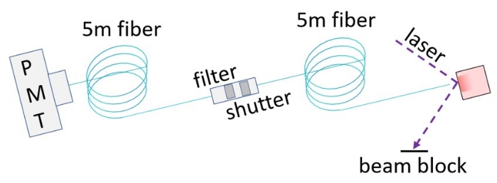
Figure 1: Schematic of the typical SPC experimental setup. Please click here to view a larger version of this figure.

Figure 2: Schematic of the AOM optical setup for long lifetime measurements. The lenses are necessary only if the response time of the AOM needs to be minimized. Essentially, if the beam is focused onto the crystal, then less time is required for the acoustic waves to pass through the region of the crystal exposed to the laser beam. The lenses can be left out when the time bins are relatively long compared to the AOM response time. Please click here to view a larger version of this figure.

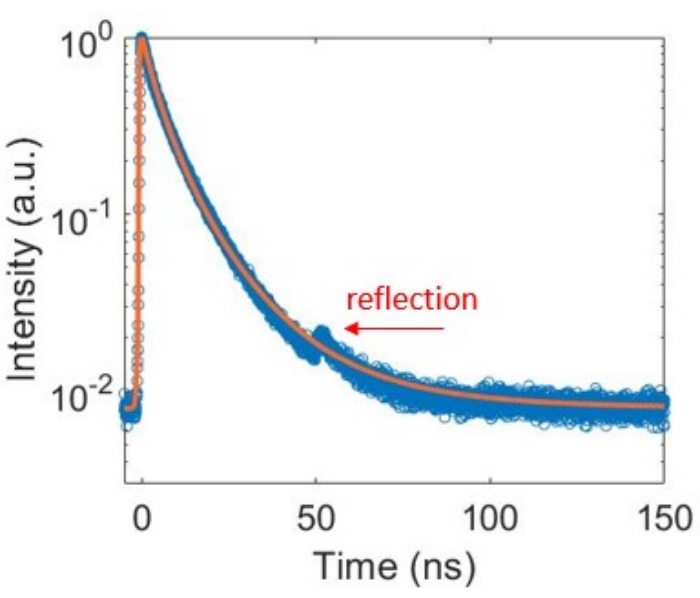
Figure 3: A fluorescence decay curve illustrating representative results. The offset in this luminescence decay is due to a long-lived phosphorescent component in the decay spectrum. Please click here to view a larger version of this figure.

Figure 4: Standard diagram of the SPCM electronic configuration. Please click here to view a larger version of this figure.

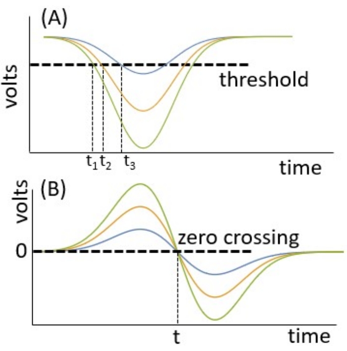
Figure 5: Diagram of the CFD amplitude and zero-crossing pulses. (A) Variable amplitude detector voltage pulses lead to timing jitter if a constant threshold discriminator is used. (B) The signal is split, one component is delayed and inverted, and then the components are recombined in the CFD. The zero crossing occurs at the same time independent of the amplitude. In practice, a threshold is used to reject the smaller noise-related pulses before the CFD is applied. Please click here to view a larger version of this figure.

Figure 6: Illustrative fluorescence decay curves. The effect of sync delay or pulse delay on the position of the PL decay curve within the recorded time interval is illustrated. The black curve represents the ideal position. Please click here to view a larger version of this figure.

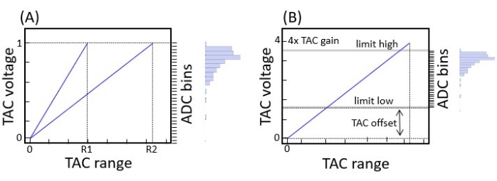
Figure 7: Effects of TAC settings. (A) Graphic illustrating two different TAC ranges R1 and R2. Range R1 is obviously shorter, the TAC ramp is steeper, and the timing resolution will be higher. (B) The same as in (A), except the TAC gain has been set to 4 times, a TAC offset has been applied (dotted lines), and ADC limits have been set (thick gray lines). Modified with permission after Reference 20. Please click here to view a larger version of this figure.

Figure 8: Illustration of the reverse stop-start counting method. The TAC starts on receiving a photon pulse from the detector (red vertical lines) and stops on the next sync pulse (black vertical lines). The times, Δt, are recorded and subtracted from the period in order to obtain the PL decay trace. Here, the delay timing (via pulse delay generator or cable lengths) is adjusted to prevent the TAC dead time from overlapping the subsequent photon pulse. Please click here to view a larger version of this figure.

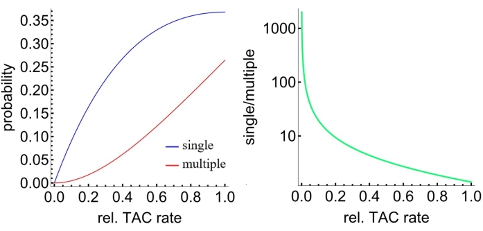
Figure 9: Poisson statistics in relation to the count rate. (A) Probability of single vs. multi-photon events within the TAC window. The relative TAC rate is equal to the TAC rate divided by the sync rate. (B) Ratio of single to multiple detection events as a function of the relative TAC rate. Please click here to view a larger version of this figure.

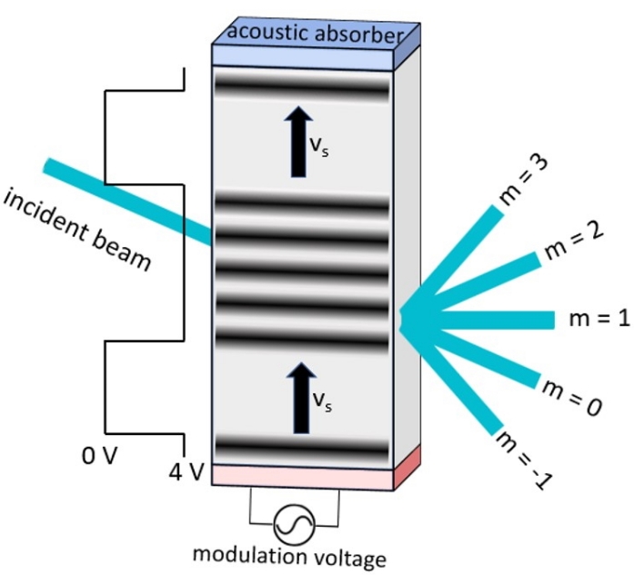
Figure 10: Diagram illustrating the grating formation in the acousto-optic crystal. A piezo (bottom) applies pressure to the AOM crystal at a built-in modulation frequency on the order of hundreds of MHz. This produces acoustic waves that travel up the crystal at the speed of sound, v_s. The timing of the piezo is controlled by the generator frequency and waveform. An interference pattern is set up when the incident beam passes through the acoustic grating. All but the m = 0 maximum will flash on and off at the generator frequency. Please click here to view a larger version of this figure.

Discussion

There are several important user-controlled parameters in any SPC setup that must be understood by the user. These parameters will explain the limitations of the SPC method for TRPL, allow the user to troubleshoot the setup more easily if something goes wrong, and help to understand the critical steps that are effectively required for good data collection. Moreover, different samples will often require different system settings - in other words, one cannot have a single procedure for all possible SPC decay traces. The setup must be modified all the time, which requires an understanding of the key elements of the system. The following discussion is with specific reference to the equipment used to gather the data in Figure 3 (see Table of Materials); however, much of the discussion is general for SPC systems.

Detector characteristics and limitations
Optimal detector characteristics for TRPL include low noise (ideally lower than 100 Hz) and an instrument response function (IRF) ideally better than 200 ps for direct-gap nanocrystals, graphene quantum dots, organic fluorophores, and any other fluorescent compound with few-nanoseconds time constants. The IRF is largely determined by the detector transit time spread (TTS), which is the variation of the time delays between the photon striking the detector and the generation of an electrical pulse at its output. The TTS is essentially the amplification time in the detector (i.e., a photomultiplier tube) and should be the main factor that controls the ultimate time resolution of the TRPL system.

In many detectors the IRF is wavelength dependent. For example, a single-photon avalanche photodiode (SPAD) showed an IRF ranging from 108 to 360 ps on changing the wavelength from 440 to 485 nm.²¹ Accurate measurement of the IRF requires it to be done near the TRPL emission wavelength, which can be accomplished using a picosecond pulsed laser to excite a suitable dye standard with ultrafast dynamics.²² Additionally, temporal broadening effects can occur due to dispersion in optical fibers or other experimental conditions. Timing jitter in the electronics can also cause IRF broadening, as discussed further below.

Hybrid PMT models can be especially nice because of the excellent sensitivity in the red and infrared for some models (useful for silicon nanocrystals) and lack of afterpulsing. Less expensive units may be uncooled and thus have a high dark count rate (up to 3,000 Hz) at room temperature. The dark noise depends on the local temperature - even 5° or 10° making a measurable difference. Therefore, an uncooled detector should always be kept as cool as possible by not having heat-producing devices (such as an Ar laser) working nearby at the same time. Regardless of the device being used, the IRF must be regularly tested in the laboratory setting in order to ensure proper operation, ideally at the PL wavelength and with the same optical path as for the sample.

The PMT used to accumulate the data in Figure 3 produces a negative voltage pulse of magnitude ~50 mV when it detects a photon (the amplified single electron response). This pulse needs to be timed down to the picosecond level by a single-photon counter module (SPCM). In SPCMs the timing resolution should be on the order of single picoseconds, so the overall response is limited by the detector IRF. The PMT output is connected to the "CFD" input of the SPCM (Figure 4). One has to be especially careful during the setup to ensure that the limit of the SPCM input is not exceeded (i.e., -500 mV), in order to not damage the SPCM hardware. Please note: it is the user's responsibility to ensure that the proper voltages are used in all apparatus. Check the manuals.

There are obviously a range of other important detector characteristics such as the bandwidth, spectral response, and amplification. These are discussed extensively in other sources^4,23,24,25. One rarely discussed limitation is the effect of the detector responsivity or quantum efficiency curve on the measured PL dynamics. This can have profound effects in cases where the luminescence is spectrally broad and, at the same time, there is a wavelength dependence of the luminescence lifetime. This situation is often the case in semiconductor nanocrystals, where inhomogeneous broadening due to the size distribution causes a wide lifetime distribution. The measured ensemble decay is affected by the response function of the detector and the resulting measured lifetimes from different detectors can be different by a factor of two¹⁶. One way to avoid this issue is to perform wavelength-resolved TRPL.

Synchronization and trigger timing: critical steps
Detection of the photon (detector) pulses in the SPCM must be timed relative to the incident laser pulses. There are two options: pick off the pulsed excitation beam with a beamsplitter and send it to a fast photodiode, which is connected to the sync input of the SPCM. The PL photons are then timed with respect to the sync pulses. Alternatively, one can sync from the internal pulse repetition frequency of the laser controller. Although there is typically tens-of-ps pulse-to-pulse timing jitter in many diode laser controllers, this may still be smaller than the IRF of the photon-counting detector. One again has to be careful with the connections - for example, many SPC modules require a negative pulse with a maximum amplitude of -500 mV; whereas laser controllers often produce much larger amplitudes. Hence, the sync signal may need to be attenuated and inverted before connecting it to the sync input of the SPCM.

Moreover, one must consider the relative timing difference between the sync pulses and the pulses from the single-photon detector. The different light paths, cable lengths, and electronics mean that the timing difference will not simply be the time between the laser pulse (the sync signal) and the photon pulse from the detector (in other words, the PL decay histogram will not start at time zero). In fact, for reasons discussed below, it can even start at a time outside the recorded data range, in which case the PL decay function will not be observed at all. Whether this happens depends on the laser pulse frequency, the time-to-amplitude converter (TAC) settings, and the relative delay time between the sync and detector pulses. This is especially important in systems using the reverse stop-start method.

There are two simple hardware methods to control or troubleshoot the time delay between the trigger and the signal pulse. One is to use different-length electronic cables connecting the sync or the PMT outputs to the SPCM. While straightforward, this method is awkward and lacks flexibility for tunable laser frequencies. Instead, a pulse delay generator can be used on the sync signal. Active pulse generators are economical although there is the risk of electronic jitter. A better choice might be a passive delay generator, but these can be more expensive. Again, the purpose of the delay generator is to make sure that the PL decay falls acceptably within the recorded time-to-amplitude converter (TAC) range for any laser repetition frequency. If the system has a fixed frequency (e.g., a Ti:sapphire laser), then one can set the delay with cable lengths and never change it afterward.

The basic electronic configuration is similar in many SPCMs (Figure 4). The two inputs - the sync pulses and those from single-photon-counting detector are first sent to their respective constant fraction discriminators (CFDs). The outputs from the CFDs are then sent to the time-to-amplitude (TAC) capacitor, which establishes the relative time difference as a voltage. This signal is then passed to the analog to digital converter (ADC), which digitizes the data for storage as a voltage (pulse timing) histogram in the system memory.

Constant fraction discriminator
There are two constant fraction discriminators (CFDs) in TRPL setups, one for the detector pulses and one for the sync pulses. The CFD is used in place of a constant threshold discriminator. The CFD triggers at a fixed fraction of the maximum pulse voltage. The idea behind the CFD is to reduce timing jitter caused by voltage amplitude variations coming from the incoming detector and sync pulses. With a constant threshold discriminator, higher pulses would reach the threshold at earlier times, causing potentially unacceptable timing jitter (Figure 5A). Pulse height variability is less likely on the sync line, so some systems may not have the sync CFD as an (easily) adjustable parameter.

The CFD eradicates amplitude jitter by splitting the input pulses in two, and then inverting and slightly delaying one of them. The pulses are then recombined and the time when the resulting sum of the two pulses crosses through zero is independent of the pulse height (Figure 5B). The discriminator level usually must be offset slightly away from zero (e.g., by -5 mV). Otherwise, with the crossing set to exactly zero, random small-amplitude pulses can cause the CFD to register a signal. The optimal CFD setting can be checked by varying the offset and checking the IRF.

The CFDs also have a threshold setting applied before the zero-crossing discriminator. The thresholds should be selected to optimally pass all signal photons and reject thermal noise pulses, and thus should be increased with increasing detector gain. In practice, one just has to look at the data; if the baseline seems high, try increasing the magnitude of the CFD threshold. Note that PMT afterpulsing (or an insufficiently dark workspace) can also cause a high baseline value.

The observed CFD frequency should always be 10-100 times lower than the sync frequency. In other words, most of the laser pulses should not have produced a detected PL photon. The reason has to do with the "pile up" issue, as discussed further below.

Time-to-amplitude converter - important considerations
The outputs from the CFDs are sent to a time-to-amplitude converter (TAC). This is a capacitor that starts charging upon the START signal and stops upon receiving the STOP signal. The magnitude of the voltage pulse from the TAC is directly related to the delay time between the start and stop pulses. The TAC frequency will be somewhat smaller than the CFD frequency because the CFD may still detect pulses while the TAC is experiencing dead time. The TAC range option sets the slope of the TAC capacitor - if the range is small, the slope will be steep and photons outside this range will not be detected. With a longer sync delay, the PL decay function moves to earlier times, and may eventually move outside the recorded TAC range. The length of the TAC range is equal to the TAC gain multiplied by the time per channel and the ADC resolution. The delay generator is used to place the decay conveniently near the left side of the recorded range, as illustrated by the black curve in Figure 6.

There are a few critical TAC settings to pay attention to. First, there is the range option. The TAC range sets the slope of the TAC capacitor charging time - it sets the time to the maximum TAC voltage (Figure 7A). The TAC range is essentially mapped into the ADC window to produce a histogram of voltages corresponding to the times between the start and stop signals. The TAC gain option multiplies the TAC output, which enables shorter time per channel to be mapped into the ADC (Figure 7B). Thus, the TAC gain should be increased if a higher timing resolution is needed.

The TAC limits (limit low and limit high) constrain the range of voltages that the TAC will output to the ADC. The limit low will always be with reference to the TAC offset as shown in Figure 7B. The limits are used to exclude early (limit high) or late (limit low) photons in the reverse start-stop configuration (or opposite in forward start-stop). Late photons may be related to detector noise and early ones could be related to the incident laser beam, for example, in case the filter did not entirely remove it, or Raman photons from the sample. With the limit low and limit high set above 0 and below 100%, respectively, a narrower range of the TAC window is mapped into the ADC histogram. This also produces a higher timing resolution.

The TAC range may need to be set to 3%-10% and 90%-97%, respectively, in order to avoid deviations from linearity that can occur near the ends of the TAC range. Finally, the TAC offset effectively changes the ADC window position relative to the TAC ramp (Figure 7B) when the gain is greater than 1. This is to ensure that the ADC range will map the sample TRPL decay function and not just the background.

Analogue-to-digital converter
The ADC divides the TAC range into (e.g., 4096) channels as a fluorescence decay measurement, effectively histogramming the TAC range into 4096 voltage bins in memory. The ADC frequency can be seen as the final detected photon frequency - that is, the number of photons + noise counts per second that contribute to the decay histogram. The ADC frequency is lower than the TAC frequency because the ADC may not accumulate the entire TAC range (e.g., Figure 7B). If many events are outside the recorded range (wasted signal), then the ADC frequency will be small and the decay will only show the background offset. By changing the delay time or TAC offset when the laser repetition frequency is low, one can effectively move the luminescence decay into the ADC's recorded interval, as illustrated in Figure 6, and a suitably high ADC signal will be recorded.

Some setups may have a sync frequency divider. This is used to record single or multiple periods. Controlled by the software, the sync frequency can be reduced by a given factor. With the divider set to factors greater than one, the sync rate is divided down internally so that several periods of the signal can be shown in each ADC recorded interval. This can be helpful when recording signals with repetition periods smaller than the minimum TAC range. With the frequency divider set to 4, one might then see four PL decay functions in the ADC range and all of that data can be used for statistical purposes or when looking for the appropriate recorded interval for the ADC.

Dead time considerations
Dead time is the time required to reset the TAC and the associated electronics after a pulse has been registered. Understanding dead time and how to minimize its contribution to the data accumulation can be of critical importance. It is an important consideration in the collection of PL decay traces because it adds to the overall collection time required to achieve the desired statistics. Once the TAC receives a stop signal, the electronics must measure the voltage and reset the TAC. This dead time should be on the order of 100 ns. The larger the TAC range, however, the longer is the associated dead time. The dead time can extend into the following signal period, further reducing the data collection efficiency. The timing of the system has to be set in order to prevent the dead time from significantly interfering with subsequent photon pulses; otherwise, the data collection may become impractically inefficient. A common technique to minimize dead time is the so-called "reverse stop-start" method. It is necessary to understand this method when setting the SPCM parameters.

Reverse stop-start
Many modern SPCMs use a reverse start-stop configuration (Figure 8). This minimizes the effects of dead time. In this mode, the TAC is triggered by the detector photon pulse and the stop signal is the subsequent sync pulse - exactly the opposite to a typical user's expectation. The histogram is then reversed in the hardware or software - in other words, the time between the detected photon and the next sync pulse is subtracted from the sync pulse interval to produce a "normal" decay function.

The TAC electronics are thus only started when a photon is detected, rather than on every sync pulse. Only for those intervals in which a photon is detected will there be an associated dead time. This reduces the total dead time significantly. A photon should be detected by the TAC typically less than 5% of the time in order to minimize pile-up distortions. It should be noted that modern time-correlated single photon counting (TCSPC) systems may take other approaches that do allow forward stop-start without excessive deadtime by incorporating multiple independent timing channels.

Limiting background signals due to afterpulsing
Afterpulses are spurious detector events that can occur over different timescales depending on the mechanism involved. Short-delay afterpulses (nanosecond regime) are due to electrons scattered elastically from the first PMT dynode. Alternatively, one can also get afterpulses coming from ionization of residual gas molecules in the PMT tube, and these appear on a time scale from hundreds of ns to microseconds after the primary pulse. Even solid-state detectors such as single-photon avalanche diodes can suffer from afterpulsing. In high-frequency experiments, the highly-delayed afterpulses can accumulate into a steady-state background signal. Afterpulsing can be reduced by lowing the detector gain a little, but then one may also have to lower the CFD threshold and end up more sensitive to dark noise. So-called "hybrid" PMT detectors are reported to suffer from almost no afterpulsing, however.

Removing reflections
Reflections can present problems in TCSPC measurements. Optical fibers are used to collect the PL and send it to the PMT. Small "echoes" of the decay curve can be observed at a delay time equal to the time it takes light to travel twice the length of the optical fibers. This occurs because roughly 4% of the PL is reflected from the glass-air interface at each end of the fiber. The PL light traveling down the fiber reflects to the "front" of the fiber, where ~4% is again reflected back down the fiber to appear as a small secondary peak having around 0.16% of the main intensity.

To minimize this problem, long lengths of fiber will force these reflections out to longer times after the primary decay, so that they may not interfere with the decay function (and fitting algorithm) or may even be pushed out of the TAC window altogether. Other optical surfaces can lead to additional reflections, including cuvette faces and the surfaces of optical filters (see the note after step 2.6). The only way to get rid of these reflections is to design the optical setup to specifically avoid them as much as possible, or at least move them out of the time window associated with the decay trace.

Laser frequency and pile-up distortion
A high laser pulse frequency is almost always beneficial because it increases the overall count rate and minimizes data collection time. However, the pulse period needs to be at least ten times longer than the characteristic decay time of the sample in order to fully capture the decay trace - otherwise the subsequent pulse will arrive before the previous decay is completely finished and this can complicate the modeling of the decay function.

Using lower-than-required frequencies has significant drawbacks, however. Obviously, it increases the data collection time, but in addition it means that one may have to install a delay line or pulse delay generator in order to ensure that the PL decay falls within the recorded interval. Moreover, it increases the probability that a start pulse will be initiated by noise - either a dark pulse or a stray photon. For a detector with poor noise characteristics, the noise problem can become so severe at frequencies below 100 kHz that one may not see any decay function at all, because almost every TAC interval is started by detector noise. Low noise detectors are thus important when low frequencies must be used.

During measurement, the TAC rate must be kept smaller than, at most, 10% of the sync rate. This value appears to be an accepted "rule of thumb" although 5% is preferable and generally not difficult to achieve. The photons follow Poisson statistics, so if the TAC rate were, for example, equal to the sync rate (average of one detected photon per laser pulse), one would get multiple photons within the TAC interval nearly as many times as one would get a single photon (26% vs. 37%). However, only the first photon within the interval can be recorded by the TAC, both for forward and reverse start-stop SPC systems. This means that the second photon is invisible to the SPCM, causing the data to become biased toward the earlier photons and the decay to appear faster than it really is. By keeping the TAC rate to less than 5% of the sync rate, one gets a single photon ~40 times more often than multiple photons within the TAC range (Figure 9).

Moreover, at high count rates, it is possible for two photons to arrive within the single-electron response time of the detector, registering as a single strong pulse. These multiphoton events can be identified by setting the CFD threshold to a higher value. Since this distortion is associated with the detector and not the TAC electronics, the only way to minimize it is to reduce the PL emission.

Count rate considerations
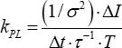
As discussed above, one typically wants the TAC count rate to be at most 5% of the sync rate when collecting the PL decay trace, in order to minimize pile up distortion. The PL count rate measured by the TAC, k_PL, has been estimated as:¹⁰

(1)

in which σ is the desired relative statistical error of the lifetime measurement, ΔI is the range of signal strength over which the decay is measured (i.e., the ratio of the maximum PL intensity to the minimum intensity in the decay), Δt is the time per histogram bin, τ is the PL decay lifetime (assuming a single exponential), and T is the total acquisition time. Imagining that one wants to determine the decay constant (τ ^-1) to within 1 part in 20, so σ = 0.05, the time windows are Δt = 12.2 ps and the TAC gain is 1, the specimen decay time constant is 1 ns, a factor of ΔI = 500 between the largest and smallest count number is required, and the collection time is 10 min, then one obtains k_PL = 27 kHz, which will be the TAC frequency if every photon is detected (i.e., with no reductions due to dead time). The laser frequency must therefore be at least 5.4 MHz in order to meet these requirements while minimizing pile-up events to less than 1/40 of the total signal.

Long lifetime TRPL
Silicon nanocrystals present an excellent example in which the lifetime is typically on the order of tens to hundreds of microseconds. Such a long decay enforces extremely low laser pulse frequencies on the order of hundreds of Hz. Phosphorescent organic dyes (triplet decay) have a similar issue. The SPC systems described above will obviously not work under these circumstances.

To detect such long PL decay traces, an entirely different setup is needed, starting with a controllable low-rep rate pulsed laser or the conversion of a continuous wave (CW) beam to a pulsed one. One advantage of starting with a CW laser is that the laser pulse function can be entirely controlled, from narrow pulses to square waves or even sine waves for frequency-resolved spectroscopy. One can use an acousto-optic modulator (AOM), an electro-optic modulator (EOM), or a chopper wheel to obtain the pulsed beam. Of these, an AOM gives excellent performance and versatility for the price. EOMs are also excellent but tend to be more expensive. A chopper wheel is a "brute-force" method, which is not recommended anymore for TRPL spectroscopy due to its poor rise time characteristics, local noise generation, and lack of flexibility in selecting the desired waveform.

Briefly, the AOM sets up a periodic interference grating by using a piezo crystal to create sound waves in an internal acoustic crystal (i.e., TeO₂, SiO₂, etc., depending on the desired wavelength range), causing a periodic variation in the index of refraction (Figure 10). This grating is switched on and off by the waveform generator that drives the piezo controller. The laser beam will form an interference pattern when the beam passes through the acoustic grating. The AOM has a built-in frequency (tens or hundreds of MHz) used to generate the grating. Thus, there are two frequencies: a user-controlled one that determines the frequency of the diffracted beams and an internal frequency for producing the acoustic vibrations. The timing resolution is set by the acoustic wave speed, v_s, and the incident laser spot size. Thus, the beam must be focused into the AOM if a the shortest risetime (a few nanoseconds) is required.

While the operating details of the AOM can be found in technical papers and application notes^26,27, here just a few practical points about alignment and timing resolution are presented. During the alignment, the user should make sure that roughly 50% the overall laser power is found in the main diffracted beam. For alignment, it is easiest to select a low drive frequency easily visible to the eye. The initial setup (Figure 2) can be tricky, because at first one may not see any diffracted beams at all. The diffraction efficiency is extremely sensitive to the direction and angle of the incoming laser beam. This can require a lot of tweaking to get the angle "just right". One wants to walk the beam into the input hole exactly horizontally and along the surface normal of the AOM. The AOM should sit on at least a 2-axis goniometer stage allowing "roll and yaw" of the AOM with respect to the incoming beam. Once the diffracted beams become visible, one has to adjust the alignment until the brightest diffracted beam has around half of the optical power. All the other beams are then blocked with an iris.

For silicon nanocrystals, one should use an infrared-optimized detector. The sync from the waveform generator and the pulse output should be interfaced to the appropriate inputs for the multichannel scalar (MSC). The time bins can be set from ns to milliseconds or longer in these setups. The counting is, in this case, started by the sync and will stop at the end of the recorded interval. The system waits for the next sync input to begin recording again.

An advantage of the MSC is that, unlike a CFD-TAC system, it can accept multiple photon pulses for a single start signal. In other words, it can register multiple distinct events, even thousands of photon arrival times per pulse. The trade-off is that the timing jitter is much worse, but if one is measuring in microsecond time windows (as opposed to nanoseconds), then this jitter is acceptable. This is why the MSC system is useful for very low repetition rates and is not as susceptible to detector noise compared to CFD-TAC systems.

Conclusion
TRPL is a key experimental method for the study of semiconductor nanocrystals and light emitting materials in general. Much information can be gained by performing high-quality, repeatable experimentation and appropriate data analysis and model fitting. Single photon counting setups are becoming ubiquitous and are now probably the standard way to measure PL decays. Unlike more complicated ultrafast setups such as optical Kerr gating, SPC systems are easy to set up, commercially available as complete units, if desired, and are becoming increasingly affordable for everyday lab use. However, many students of TRPL are not familiar with the setup considerations and may be faced with having to sort through a huge amount of information⁵ in order to try to understand what is really going on, what the limitations are, how to avoid artefacts, and how to collect optimal data in a reasonable period of time.

This paper was intended as a "how to" discussion for the experimental student of TRPL. The focus is on the equipment reported in this paper, but many of the points are generally applicable to most or all SPC systems for TRPL. The procedure gives specifics of how to build and use a SPC setup for TRPL, but there can be many variations on this procedure depending on the equipment used and the sample to be measured. The relatively long discussion was meant to outline the elements that the user must understand in order to be able to get good data, coming from a few years of sometimes frustrating personal experiences.

While several works have presented many of the issues associated with the model fitting of TRPL decay functions, there are relatively few recent papers dealing with basic experimental SPC setup and control for TRPL. The intent of this paper was to outline the practical aspects for conducting good TRPL experimentation, to review the key considerations when performing TRPL, and to serve as a quick reference guide for how to set up and perform TRPL experiments over a wide range of timescales.

Materials

List of materials used in this article

Name	Company	Catalog Number	Comments
AOM	Isomet	1260C
Laser	Alphalas	Picopower
Laser	Coherent	Enterprise
MCS	Becker-Hickl	PMS-400
PMT	Becker-Hickl	HPM100-50
PMT	Hamamatsu	H-7422
SPCM	Becker-Hickl	EMN130