A Comprehensive Protocol and Step-by-Step Guide for Multi-Omics Integration in Biological Research

Summary

This work details methods for integrating multi-omics data (concatenation, transformation, and model-based). By combining data from genomics, epigenomics, transcriptomics, proteomics, metabolomics, metagenomics, lipidomics, and glycomics, a comprehensive understanding of biological systems is achieved. The manuscript provides step-by-step guidelines, highlighting limitations, advantages, and visualization tools for multi-omics integration.

Abstract

This manuscript provides a comprehensive step-by-step guide for integrating multi-omics data in biological research.

Multi-omics data integration refers to the process of combining and analyzing data measured on the same set of biological samples with different omics technologies, such as genomics, epigenomics, transcriptomics, proteomics, metabolomics, microbiomes, lipidomics, and glycomics. Even though multi-omics approaches have similar objectives as single-block or single-omics analyses (for instance, description, discrimination, classification, or prediction), they are able to capture a broader spectrum of molecular information, thus providing a deeper understanding of biological systems and their complex interactions. Indeed, the combination of multiple-omics datasets enables the improvement of prediction accuracy and yields more robust results, especially in cases where the number of available samples is limited. Moreover, thanks also to the most recent development of machine learning techniques, multi-omics analyses are nowadays suitable to uncover hidden patterns and complex phenomena arising among different biological compounds.

The primary aim of this work is to present the full protocol that is commonly used in multi-omics studies, from the initial formulation of the problem to the tools useful for the biological interpretation of the results. The manuscript describes in detail the various methods of integrating multi-omics data, including concatenation-based (low-level), transformation-based (mid-level), and model-based (high-level) approaches, and highlights their limitations and advantages, along with the presentation of general visualization and diagnostic tools.

Introduction

The field of biological research has witnessed significant advancements in recent years, particularly in the area of omics technologies. These technologies provide valuable insights into the complex nature of biological systems. However, each omics technology offers a unique perspective on biological components, necessitating the integration of multi-omics data to obtain a comprehensive understanding.

Multi-omics encompasses various classes of biomolecules that can be quantitatively defined thanks to the advent of new and powerful high-throughput sequencing techniques. Among the different types of omics technologies are genomics, epigenomics, transcriptomics, proteomics, metabolomics, metagenomics, lipidomics, and glycomics. Genomics involves the study of an organism's genomes, while epigenomics focuses on the supporting structure of the genome, including protein and RNA binders, alternative DNA structures, and chemical modifications on DNA. Transcriptomics encompasses the study of all RNA molecules, including mRNA, rRNA, tRNA, and other non-coding RNA. Proteomics involves the study of proteins, including modifications made to specific groups of proteins. Metabolomics focuses on the ensemble of small molecules (metabolites) within a biological matrix. Metagenomics involves the study of microbial communities in well-defined habitats with specific physico-chemical properties. Lipidomics encompasses the study of the entire complement of cellular lipids, while glycomics focuses on the study of the glycome, including carbohydrates and sugars¹.

The integration of multi-omics data has gained increasing attention in the scientific community due to its potential to unravel complex biological phenomena. By combining data from multiple omics technologies, researchers can overcome the limitations of individual datasets and gain a more holistic view of biological systems. This integrated approach enables the identification of novel biomarkers, the discovery of disease mechanisms, and the elucidation of intricate biological pathways.

The number of citations of the terms "Multiomics" and "Multi-omics" in PubMed has significantly increased over the years, from 307 in 2018 to 1414 in 2021 to 3933 in 2023. The integration of different types of omics variables is becoming increasingly common as it allows for a deeper investigation into the mechanisms underlying diseases and dysfunctions of organisms. Single omics approaches provide a limited, partial view of the hidden biology, as they focus on a single perspective. However, by integrating multi-omics data, we can shed light on the interplay of different biomolecules, understanding the relationships within multiple layers, and bridging the gap between genotype and phenotype. Overall, multi-omics approaches can help answer important questions such as classifying different subgroups of diseases, predicting fundamental disease-associated biomarkers, and gaining a better understanding of biological pathways and mechanisms. In the following sections, the different omics datasets can also be referred to as data "views" or data "blocks".

Techniques for multi-omics integration can be classified into three main subgroups, as described by Reel et al. (2021)² and Ritchie et al. (2015)³ (Figure 1).

Low-level, early integration or concatenation: This approach involves concatenating variables from each single dataset into a single matrix. However, early integration does not consider the unique distribution of each omics data type and may assign more weight to certain omics data types with larger dimensions. It also poses challenges such as an increased risk of the curse of dimensionality, added noise, highly correlated variables, and computational scalability issues. Despite these limitations, early integration allows for the identification of coordinated changes across multiple omic layers and enhances biological interpretation.

Mid-level, middle integration or transformation-based: In this approach, mathematical integration models are applied to the multiple layers of omics data. Middle integration focuses on the fusion of subsets or representations extracted from the sources. Two sub-approaches within middle integration are the middle-up approach and the middle-down approach. The middle-up approach involves concatenated scores obtained from dimensionality reduction on each block, making it suitable for handling heterogeneous data. However, it may lack interpretability. The middle-down approach involves local variable selection and subsequent analysis on concatenated variable subsets, allowing for easier interpretation of the models. Middle integration offers advantages such as improved signal-to-noise ratio, reduced dimensionality, and improved statistical power.

High-level, late integration or model-based: This approach involves performing analyses at each single omic level and combining the results in an ad-hoc fashion. It includes the fusion of results from single block models to identify biomarkers from each source and provide a joint interpretation of the results. Late integration does not increase the dimensionality of the input space and works with the unique distribution of each omics data. It is particularly appropriate when one omic layer is more predictive than others. However, late integration may overlook cross-omics relationships and face challenges related to the lack of understanding of the connections between initial data blocks and the potential loss of biological information through individual modeling.

Protocol

1. Research question(s) definition

1. Clearly articulate the specific research question(s) that will be addressed through multi-omics integration. E.g., Research question 1: What are the changes in protein expression and metabolite profiles that correlate with treatment response? Research question 2: How do genetic variations influence gene expression patterns in patients with a given disease? Research question 3: How does the integration of specific omic layers provide a comprehensive understanding of a specific biological process or disease mechanism?
2. Consider the inclusion of multiple omics technologies to search for biomarkers or gain mechanistic insights into complex diseases. Note that increasing the sample size may be necessary for patient stratification.

2. Omics selection

1. Identify the most relevant omics technologies for the research question(s) and the biological system under study. For example, in the case of question 1, the relevant omic technologies are proteomics and metabolomics; for research question 2, genomics and transcriptomics; and for research question 3, several omic technologies.
2. Consider the purpose of the study and available resources when choosing the ideal omics layers. Examples include metabolomics for nutritional research, genomics and transcriptomics for cancer biology, and proteomics for various diseases.

3. Ensuring data quality

NOTE: Ensure data reliability and reproducibility of the omics data generated following the steps described below.

1. Carefully design the experiment and maintain consistent experimental conditions and sample collection methods across all omics layers to minimize batch effects.
2. Follow established protocols and implement quality control measures during data generation for each omic dataset.
   1. Use internal or external standards when appropriate.
   2. Perform quality checks in individual omics datasets.
      1. For genomics data, assess metrics such as read quality scores, base composition, and sequencing depth to ensure high-quality sequencing data, as well as alignment and mapping quality and variant calling quality, including allele frequency, read depth, and variant annotation.
      2. For transcriptomics data, assess metrics such as read length distribution, base composition, and Phred quality scores when assessing read quality, and transcript per million (TPM) or fragments per kilobase of transcript per million mapped reads (FPKM) when assessing transcript quantification quality.
      3. For proteomics data, consider relevant metrics such as peak intensity distribution, signal-to-noise ratio, and mass accuracy when assessing mass spectrometry data quality and peptide sequence coverage, protein identification score, false discovery rate, and reproducibility of protein abundance measurements when assessing protein identification and quantification quality.
      4. For metabolomics data, assess relevant metrics like peak intensity distribution, signal-to-noise ratio, and mass accuracy when assessing mass spectrometry data quality and matching mass spectra with reference databases or using fragmentation patterns for structural elucidation when evaluating metabolite identification quality.

4. Data preprocessing

1. Overlapping samples
   1. Include only samples that overlap across multiple omics datasets.
   2. Exclude blocks with an insufficient number of overlapping samples compared to other blocks.
2. Missing value imputation
   1. Handle missing values using statistical or machine learning methods.
   2. Employ techniques like the Least-Squares Adaptive (LSA) method for missing value imputation.
   3. Avoid removing rows with missing data, especially when dealing with limited samples.
   4. Exclude variables with a high percentage of missing values (e.g., 25% or 30% missing values across samples).
3. Standardization
   1. Perform data manipulation to ensure consistent scaling of features.
   2. Prevent features with larger effects from dominating those with smaller effects.
   3. Apply common transformations like logarithmic transformation, centering, and scaling.
      NOTE: Transformations should be carefully chosen to maintain the interpretability of the original data.
4. Outlier identification
   1. Detect outliers and extreme values using tools such as boxplots or distance from the median of the values.
   2. Address outliers through appropriate methods such as data transformation or removal.

5. Dimensionality reduction

NOTE: There are two approaches to dimensionality reduction: the removal of noisy and redundant variables (feature selection) or the combination of features to create more meaningful variables (feature extraction).

1. Identify if the aim of the study is predictive (e.g., build a model able to predict if a subject is healthy or sick) or analytic (e.g., which variables are biomarkers of a disease).
   NOTE: If the aim of the study is analytic, feature selection is more appropriate because feature extraction may result in loss of interpretability.
2. When dealing with highly dimensional data, it is important to select relevant variables to the phenomenon studied to ease the analysis and interpretation, reduce the computational resources needed, and remove noise and redundant information that will confound the results.
3. Feature selection
   1. Identify the subset of informative features for the phenomenon of interest.
   2. Use feature selection methods classified into categories such as filter, wrapper, embedded, and hybrid methods. In the case of multi-omics, biomarker selection methods can also be applied.
      NOTE: Consider the dataset characteristics when choosing the appropriate method. Wrapper methods provide the most accurate prediction models, but they require a much longer computation time than filter or embedded methods. A summary table with advantages and disadvantages of different feature selection and extraction methods is provided in Table 1.
   3. Balance the performance of the final model with the computational effort required for feature selection.
   4. Optimize the number of selected features to avoid underfitting or overfitting.
      NOTE: Examples of overfitting risks are discussed in a previously published work.
   5. Evaluate the model's performance using metrics such as accuracy, area under the curve (AUC) score, or balanced error rate (BER).
4. Feature extraction
   1. Transform raw data into a reduced set of meaningful features:
      1. Apply techniques like Principal Component Analysis (PCA) to identify important patterns and relationships by projecting data onto a lower-dimensional space.
      2. Utilize t-SNE for visualizing high-dimensional data while preserving local similarities.
      3. Consider Linear Discriminant Analysis (LDA) to maximize class separability.
      4. Explore Autoencoders to learn compressed representations of the data using neural networks.
         NOTE: Feature extraction may result in representations that are harder to interpret. Table 1 lists selected examples of feature selection and feature extraction methods⁵.

6. Integration method selection

1. Identify the most relevant(s) integration method(s) to apply to the data.
   1. If samples are matched and there are enough complete subjects, then proceed with an early integration method.
   2. If inter-layer interactions must be taken into account, then do not proceed with a late integration method.
   3. If signals may be subtle but consistent across layers, then an early integration method may be more suitable than a late integration method.
   4. If it is important to leverage the interrelationship of data between the different omic layers, then choose a middle integration method.
   5. Low-level integration of concatenation
      1. If one (or more) of the omics blocks remains much larger in number of features (variables) than the rest, reduce its (their) dimensionality following the steps in section 5.
      2. Concatenate variables from each single omics dataset into one wide matrix.
      3. Transform concatenated variables so that they will have similar ranges and distributions.
      4. Use the concatenated data matrix for subsequent analysis, such as applying machine learning algorithms or dimensionality reduction strategies.
         NOTE: The most common way to perform low-level integration is through concatenation. However, these methods may result in the loss of relationships between blocks or block-specific insights.
2. Mid-level integration
   1. Choose from the six main categories of mid-level integration depending on the goal of the analysis.
      1. Similarity-based: Use this approach to assess similarity between different samples or features to identify patterns or subtypes within diseases, in exploratory data analysis where relationships are not known a priori. Example: SNF⁶.
      2. Correlation-based: Employ this method to identify and quantify associations between different variables, in particular to assess how one variable changes with the changes in another one. Example: CNAMet⁷.
      3. Network-based: Use network-based methods to represent complex relationships among features. It is particularly useful to uncover clusters within the data structure and predict biomarkers. Examples: NetICS⁸, PARADIGM⁹, scMoMtF¹⁰.
      4. Bayesian-based: Use this approach to incorporate prior knowledge into the analysis or when dealing with uncertainties in the data. It is particularly useful for inferring disease subtypes and predicting biomarkers based on probabilistic models. Examples: MOFA¹¹, iClusterPlus¹².
      5. Multivariate-based: Use this method to analyze multiple variables simultaneously, especially when interactions among these variables are essential for understanding the biological system. It is useful for both clustering and biomarker discovery. Examples: mixOmics¹³, JIVE^14,15_.
      6. Fusion-based: Use this method to combine data from different omics layers into a single framework to leverage the strengths of each type of data. It is particularly useful for comprehensive analyses that require the integration of diverse datasets. Examples: PFA¹⁶, PSDF¹⁷.
         NOTE: Based on strong statistical processing or modeling by machine learning techniques, it might limit issues that are present in the case of Low- or High-level integrations.
   2. Apply the selected method to the multi-omics dataset.
3. High-level integration
   1. Perform a full data analysis on each single omic block independently.
   2. Jointly interpret the results obtained in the previous step.

7. Statistical analysis

1. Differential expression (DE) analysis
   1. Prepare the data by ensuring that the data is properly formatted and normalized.
      NOTE: Depending on the packages used, the data format and structure may differ. Using R packages such as limma¹⁸, edgeR¹⁹, or DESeq2²⁰ for DE analysis is recommended.
   2. Construct a design matrix that includes separate coefficients for each experimental group, specifying the experimental conditions and group assignments.
   3. Implement a linear model and apply it to each feature, incorporating the design matrix.
   4. Calculate moderated t-statistics and F-statistics to assess differential expression.
   5. Use empirical Bayes moderation of standard errors to estimate log-odds of differential expression.
   6. Determine significance thresholds
      1. Consider a p-value cutoff of 0.05 to determine statistical significance.
      2. Set log-fold change thresholds based on the type of feature:
      3. For metabolites and proteins, use a log-fold change of log2(1.1).
      4. For transcripts, use a log-fold change of log2(1.5).
2. Clustering
   1. Select a clustering method/algorithm to use.
      NOTE: There are clustering algorithms specifically designed for multi-omics data, such as NEMO²¹, iCluster²² and JIVE²³.
   2. Determine the number of clusters if the method requires it. Some alternatives are the elbow method, silhouette score, or gap statistic to estimate the optimal number of clusters.
   3. Run the selected clustering algorithm on the cleaned data.
   4. Optimize algorithm-specific parameters as needed.
   5. Assess the quality of the clustering results using internal or external validation metrics, such as the silhouette score or adjusted Rand index.
   6. If appropriate and feasible, validate cluster assignment using independent data or a test dataset previously excluded from the cluster analysis.
3. Predictive modeling
   1. Evaluate the need to perform predictive modeling in a multi-omics study.
      NOTE: Predictive models can be applied after multi-omics integration to compare how the accuracy of prediction on the outcome classification changes based on the features selected by different methods.
   2. If the decision taken in step 7.3.1 is positive, then proceed with the following steps; otherwise, go to step 8.
   3. Choose a suitable predictive model to apply.
      NOTE: An example of a model to use is Random Forest (RF), a machine learning algorithm that integrates multiple decision trees to obtain a final result.
   4. Fine-tune model parameters (e.g., using the R caret package).
   5. Split the dataset into train and test (60-40% or 80-20%), in a balanced way to have same proportion of samples from different groups.
   6. Run the model on the train set.
   7. Compute accuracy and F1 score in the test set for evaluating model performance.
   8. Repeat steps 2 to 4 multiple times (e.g., 1000) to increase randomness.
   9. Compute the average of the results of step 5.
   10. Report averaged Accuracy and F1 score. If not satisfactory, proceed to step 1 to improve the parameter selection.
   11. Determine feature importance using mean decrease in accuracy (DMA) and mean decrease in impurity (MDI).

8. Biological interpretation:

1. Select a pathway enrichment tool (commonly used PEA tools are DAVID, GSEA, Enrichr, and Metascape).
2. Input the list of genes or proteins into the selected pathway enrichment analysis tool.
3. Select the appropriate pathway database, such as KEGG, Reactome, or GO, to perform the analysis.
   NOTE: One tool that has been specifically designed for multi-omics data is Paintomics, which uses databases (KEGG, Reactome, or Mapman) to provide information about the functional relationships between these biomarkers, as well as their involvement in specific biological processes²⁵.
4. Run the pathway enrichment analysis using the selected tool and database.
5. Adjust parameters as needed, such as significance threshold, background list of genes, or correction method.
6. Visualize and evaluate final results (enriched pathways, FDR, pathway diagrams, heatmaps, among others).

9. Validation and follow-up experiments

1. Technical validation
   1. Verify that when using different analytical techniques on the same samples, equivalent results are also found.
      NOTE: For example, results obtained using Mass spectrometry (MS)- based proteomics can be later validated using an immunological assay such as enzyme-linked immunosorbent assay (ELISA).
2. Identify follow-up experiments to validate obtained results.
3. If possible, replicate the finding by analyzing omics data from an independent cohort.
4. For clinical applications, conduct randomized clinical trials to demonstrate the clinical validity of the findings.
   1. Design and implement a controlled study with an appropriate sample size and randomization to evaluate the efficacy and safety of the identified biomarkers or targets.
   2. Collect relevant clinical endpoints and measure the impact of the identified factors on patient outcomes.

10. Visualization and diagnostic tools

NOTE: Various types of plots can be utilized to illustrate the results of data analysis, providing visual representations of key findings. Commonly used plots include Volcano plots, heatmaps, circos plots, and Manhattan plots.

1. Volcano plots:
   1. Use Volcano plots to summarize differential expression analysis (DEA) results.
   2. Display the relationship between statistical significance and magnitude of change between tested groups.
   3. Identify key features for further examination based on their position in the plot.
2. Heatmaps:
   1. Utilize heatmaps to visualize the magnitude of a variable across different categories.
   2. Use colors to indicate the intensity of the variable, facilitating the identification of patterns and clusters within the datasets.
3. Manhattan plots:
   1. Employ Manhattan plots to efficiently summarize the results of DEA and visualize numerous data points on the same plot.
   2. Commonly used in Genome-Wide Association Studies (GWAS), but also applicable in multi-omics studies.
4. Circos plots:
   1. Use circos plots, circular visualizations, to explore interactions and correlations between various molecular features.
   2. Depict relationships and connections between different elements in a comprehensive and visually appealing manner.
      NOTE: This study provides examples of Representative Results for each plot type presented above using a cancer test dataset.
5. Diagnostic tools:
   NOTE: Visualization tools, together with performance metrics, are very important for diagnostic purposes.
   1. Utilize receiver operating characteristic (ROC) curves to assess the performance of classification models.
   2. Use loading plots and principal component analysis (PCA) plots to visualize the relationships and patterns within the data.
      NOTE: Examples of representative results for each of these plots using a cancer test dataset are shown in the Representative Results section.
6. Performance metrics for binary classification
   NOTE: The following metrics can all be adapted for multi-class classification, such as in the presented example, by considering each class versus the rest, for each class.
   1. Confusion matrix: Use a confusion matrix (Table 2) to indicate the true positives and true negatives in the diagonal, true negatives in the right bottom blocks, false positives in the right top blocks, and false negatives in the left bottom blocks.
   2. Precision: It is the proportion of positive identifications that were correct. Calculate precision using the formula, TP/(TP + FP). A model with a precision of 1 has no false positives. If a model has a precision of 0.5, then the model is correct half of the time.
      
   3. Recall or sensitivity: Also known as true positive rate or hit rate, it is the proportion of actual positives that were identified correctly. Calculate recall or sensitivity using the formula, TP/(TP + FN) or TP/pos, where pos = TP + FN is the total number of positive examples.
      
   4. Specificity: It is the proportion of actual negatives that were identified correctly. Calculate it using the formula, TN/neg, where neg = TN + FP is the total number of negative examples.
      
   5. Accuracy: Proportion of correct predictions (both positive and negative). Calculate accuracy using the formula:
      
   6. F-Score: F-Score is the harmonic mean between recall and precision. Calculate it using the formula:
      
   7. Balanced accuracy: The balanced accuracy (BAC) is the average of the sensitivity and the specificity. Calculate it using the formula:
      
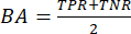
      where TPR stands for True Positive Rate and corresponds to recall, and TNR stands for True Negative Rate and corresponds to specificity.
   8. Balanced error rate: The balanced error rate (BER) is the average of the errors on each class. Calculate it using the formula:
      
      NOTE: The BER has the advantage of considering the difference in performance between the classes by creating a balanced measure of the error rate, thus limiting the effect of an unbalanced dataset. An error rate of 0.5 represents a similar performance to random guessing. For DIABLO, the BER is the weighted classification error rate from each block, depending on the correlation between the components and the condition of interest. BER is the complement of BA to 1, i.e., BER = (1 - BAC).
   9. Area under the curve: Compute the area under the curve (AUC) as the area below the ROC (described in the following section), obtained by plotting the sensitivity versus the specificity.
      NOTE: Which of these metrics is best suited for the task depends on the importance of false negatives and the balance or imbalance between the classes. Precision focuses on minimizing false positives, while recall focuses on minimizing false negatives. If there is a low proportion of positive cases, then precision alone may not be the best indicator to assess the performance of a model. Code.R is provided as Supplementary File 1.

Results

As in single-omics analysis, visualization is key for data exploration, data integration, pattern recognition, hypothesis generation, and communication of results. Specifically, good visualization of large data is very important during data pre-processing steps, aiding in the verification of normalization, identification of outliers, and many more. In multi-omics, even more so, visualization is vital, as it can aid in the evaluation of trends in the different omic layers/blocks, and the overlaying of information from eac...

Discussion

Identifying the most relevant omics dataset is one of the first steps in a multi-omics integration study. In nutritional research, metabolomics represents one of the first omics layers to look at, since it can highlight the metabolic pathways and biochemical processes at the basis of dietary intervention or metabolic response to food intake. On the other hand, for example, in cancer biology, genomics and transcriptomics which give information about DNA, genetic variants, and gene expression dysregulations, can help under...

Materials

List of materials used in this article

Name	Company	Catalog Number	Comments
Apple M2 Pro macOS	Apple	14.3 (23D56)	Processing computer
ggplot2 R package	r-project.org	3.4.4	Create data visualizations
ggpubr R package	r-project.org	0.6.0	Create publication ready plots
ggrepel R package	r-project.org	0.9.5	Automatically position non-overlapping text labels with ggplot2
lattice R package	r-project.org	0.22-5	Tellis graphics for R
limma R package	r-project.org	3.58.1	Linear models for microarray data
mixOmics R package	r-project.org	6.25.1	Omic data integration project
NEMO R package	r-project.org	0.1.0	Neighbourhood-based multi-omics clustering
R	r-project.org	4.3.2 (2023-10-31)	Programming language for statistical computing and graphics
R Studio	RStudio	2023.12.1+402 (2023.12.1+402)	Integrated development environment for R
SNFtool R package	r-project.org	2.3.1	Similarity network fusion
tidyr R package	r-project.org	1.3.1	Tidy messy data
yardstick R package	r-project.org	1.3.0	Tidy characterizations of model performance