A Quantum-Classical Hybrid Model for Long-term Network Traffic Prediction

Summary

QTSMixer, a hybrid quantum-classical model, enhances network traffic prediction by addressing TSMixer's limitations in periodic signals and long-term forecasts. It introduces quantum neural network components controlled by trainable parameters , outperforming TSMixer by 6.72% in long-term predictions on real-world data.

Abstract

Network traffic prediction, a critical application of time series analysis, is essential for network management and optimization. Traditional statistical models and machine learning methods have been employed for network traffic prediction, where recent advancements in multi-layer perception mixer architectures, particularly TSMixer, have achieved state-of-the-art performance. However, TSMixer faces challenges with periodic signals and long-term predictions. To address these limitations, we propose a Quantum TSMixer (QTSMixer) model, a hybrid quantum-classical approach that leverages quantum neural networks for enhanced feature extraction related to periodic signals and long-term dependencies. By introducing trainable parameters to control the strength of the quantum components, the hybrid structure of multi-layer perception and quantum neural network is generated. QTSMixer's cross-domain application potential and practical application capability are demonstrated through empirical analysis on real-world datasets, in which QTSMixer outperforms TSMixer by 6.72% in the long-term network traffic prediction dataset. In the future, the development of QTSMixer can be further explored in other fields, such as financial market analysis and weather prediction.

Introduction

Network Traffic Prediction (NTP)^1,2,3, as an essential application of time series analysis^4,5, involves analyzing historical network traffic data to identify patterns and trends, thereby forecasting future traffic changes. It is crucial for network management and optimization, as it can assist network operators in resource allocation, fault diagnosis, security monitoring, and quality of service assurance. The NTP problem has been well studied by statistical models and machine learning methods³. Recently, architectures based on Multi-Layer Perception Mixer (MLP-Mixer)^6,7 are becoming popular for NTP due to their powerful capability to capture multivariate time series dependencies. Among them, TSMixer⁸ stands out for its exceptional speed and lightweight design and has attained State-Of-The-Art (SOTA) performance on benchmark datasets⁹. TSMixer can better capture the time dependence and the correlation between features through the hybrid operation of time and feature dimensions. However, TSMixer has the following two disadvantages. First, it is not suitable for dealing with periodic signals. Periodic signals are stable, resistant to interference, and easy to analyze, making them highly valuable in communication, power systems, and control systems. Since TSMixer is based on MLP whose mathematical prototype is an aperiodic function, TSMixer is suitable for processing aperiodic signals but does not fit well when processing periodic signals. Second, it does not perform well when making long-term predictions as it is hampered by current computer memory limitations and the accumulation of errors in predicting. At present, most of the models have poor performance in dealing with long-term time series prediction. This is an urgent issue that needs to be solved in the field of time series prediction. Although TSMixer has achieved good results, there is still room for improvement. Therefore, it is of great significance to seek new strategies to avoid these drawbacks.

Quantum computing¹⁰ is a new computing paradigm based on quantum mechanics laws, which can process massive amounts of data both efficiently and securely. Quantum Neural Networks (QNNs)^11,12,13 are a kind of computing model that combines quantum computing and classical neural networks, which have a wide range of applications in image processing, speech recognition, and disease prediction. They exploit the properties of quantum computing, such as superposition and entanglement, to process information and perform machine learning tasks, leading to better simulations, faster computation, or quantum advantage in terms of network performance. Recently, some approaches have been investigated in the QNN realm for time series forecasting^{14,15,16,17,18,19}. Quantum time series models can surpass traditional models in terms of prediction accuracy and computational efficiency, especially when dealing with complex multi-dimensional data. On the one hand, QNN can be expressed as a Fourier series, which is a periodic function and suitable for processing periodic signals; on the other hand, some applications of QNN in time series have been successful. Therefore, it is of great interest to explore the role of QNN in NTP, especially long-term NTP.

Protocol

QTSMixer methodology

Let be a multivariate time series of length sl and number of channels c. The multivariate forecasting task is defined as predicting future values 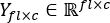given some history by a forecasting model , which can be formulated as

Where  is the forecast sequence length and denotes the prediction value. In QTSMixer, let X_L×C denote the original multivariate time series of length L and the number of channels c. We input the multivariate time series by minibatch , where sl ≤ L and b is the batch size. As shown in Figure 1, the QTSMixer model consists of four components: normalization, patch embedding, mixing layers, and forecasting. In the training phase, the loss of the model is calculated by the Mean Square Error (MSE) loss function to achieve the best fit. The QTSMixer can be characterized as

Where θ is the trainable parameter vector and is updated by stochastic gradient descent.

Figure 1: The high-level architecture of QTSMixer. Here we divide QTSMixer into four components: normalization, patch embedding, mixing layers, and forecasting. Please click here to view a larger version of this figure.

Next, we will detail the model components of QTSMixer.

Normalization

The forward propagation process of QTSMixer starts with receiving the input time series data . First, the input data are normalized and standardized by the PatchTSMixer StandardScaler⁸ or other scalers to eliminate the dimensional differences between features and ensure the stability of data performance during training.

Patch embedding

First, the standardized time series data are divided into multiple fixed-length segments (patches) through the patching module. This model design is inspired by Ekambaram et al.⁸, and the ability to capture local features is improved through the division of patches. Through patch division, QTSMixer can effectively deal with complex time series data patterns, reduce the number of model input tokens, and achieve better results in a shorter training time. The minibatch is reshaped into , where n is the number of patches and pl denotes the patch length. Let s denote the stride of patching, then .

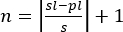To increase the expressive power of the model, each patch is mapped to a higher-dimensional space through a linear layer. Then, the data are reshaped into by linear transformation , where hf is the number of hidden features. The weight matrix has a dimension of pl × hf .

Mixing layers

In this part, the patch, feature, and channel dimensions are mixed through multiple mixing layers. Based on the dimension under focus in each mixer layer, the input is first permuted accordingly to learn correlation along the focused dimension. Then, the information is extracted by layer normalization, MLP, QNN, and Gated Attention (GA) mechanism to extract more comprehensive feature information.

In the patch mixing layer, the input is first reshaped to , in which we focus on the patch dimension (i.e., the last dimension); then, the layer normalization is performed. After that, this module employs a shared MLP (weight dimension n × n) to learn the correlation between different patches. Meanwhile, the QNN is realized by quantum re-uploading technology²⁰ to enhance the expression ability of the quantum layer. The quantum circuit in QNN has a total of ql layers, and the ith layer contains an encoding circuit U_x and an ansatz , where θ_i is the trainable parameter vector and i = 1, 2, ..., ql. Following a weighted addition operation, the model produces a hybrid structure of MLP and QNN, formulated as for the ith component of the patch dimension, to effectively integrate classical and quantum feature extraction capabilities. Note that here α_i is a trainable parameter with an initial value of 0, which indicates how strongly the quantum behavior is introduced. Finally, the GA⁸ probabilistically upscales the dominant features and downscales the unimportant features. The feature mixing layer and the channel mixing layer work in a similar way.

After multiple mixing layers, the data are processed as .

Forecasting

In the forecasting layer, the data are first reshaped to . The future values are predicted through a classical prediction head⁸—the encoded features are flattened and fed into a classical linear layer with dropout to generate a prediction of future values.

Experimental results

We conducted a detailed empirical analysis on the real-world dataset, i.e., the Long-Term Network Traffic Forecasting (LTNTF) dataset²¹, and three other popular public datasets. The first experiment is based on the LTNTF dataset²¹, which provides hourly traffic data and holiday information for three cities A, B, and C, in the real-world network from January 1, 2017, to February 20, 2019. The task is to use historical data to build an appropriate model to predict the hourly traffic values for each city for the next 95 days. The uniqueness of the dataset lies in its authenticity and long-term nature, offering detailed hourly network traffic data covering multiple cities over more than 800 days. The experimental results are summarized in Table 1, Figure 2, and Figure 3. To reproduce the experiment, refer to README.md in Experiment_1_LTNFT in Supplemental File 1.

Table 1: Performance comparison between QTSMixer and TSMixer in the LTNTF dataset. Here the MAPE and RMSE are used as the main evaluation metrics, and lower values indicate better performance. Please click here to download this Table.

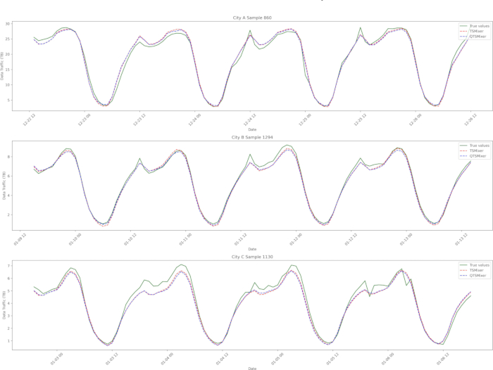
Figure 2: Comparison of prediction results of TSMixer and QTSMixer. Here we randomly select three samples from three cities and give the visual comparison between the real values and the predicted values of TSMixer and QTSMixer. Please click here to view a larger version of this figure.

Figure 3: Comparison of prediction results of a special case of TSMixer and QTSMixer. Here the samples with the best performances of QTSMixer are selected. Please click here to view a larger version of this figure.

The second experiment is based on the BasicTS+(Basic Time Series)²² framework, which is a benchmark library and toolbox for time series forecasting. It supports a variety of tasks and datasets, such as spatio-temporal forecasting and long series forecasting, and covers statistical models, machine learning models, deep learning models, and other algorithms. BasicTS+ provides a fair and comprehensive platform for the replication and comparison of popular deep learning models through a unified and standardized process. The BasicTS benchmark comprises seven carefully curated multivariate time series (MTS) datasets spanning diverse real-world domains to enable rigorous evaluation of forecasting models. The collection includes traffic datasets (PEMS04/08 for flow monitoring), energy consumption records (Electricity/Etth1/Ettm1), economic indicators (Exchange-Rate), and environmental measurements (Beijing Air Quality). The experimental results are shown in Table 2. To reproduce the experiment, refer to README.md in Experiment_2_Basicts in Supplemental File 1.

Table 2: Performance comparisons among QTSMixer and other models on various datasets of BasicTS+ framework. Here MAE, WAPE and RMSE are used as evaluation metrics, and lower values indicate better performance. The models with similar parameter counts are grouped. Please click here to download this Table.

The third experiment involves a comparative analysis between the quantum simulator and a real quantum computer. This experiment compares the performance of Qiskit and the DQ framework by evaluating their respective implementations of QTSMixer. The accuracy and execution efficiency of both frameworks in forecasting tasks were assessed. The superconducting quantum computer, ibm_brisbane, is used in this experiment. The experimental results are shown in Figure 4 and Table 3. To reproduce the experiment, refer to README.md in Experiment_3_Qiskit in Supplemental File 1.

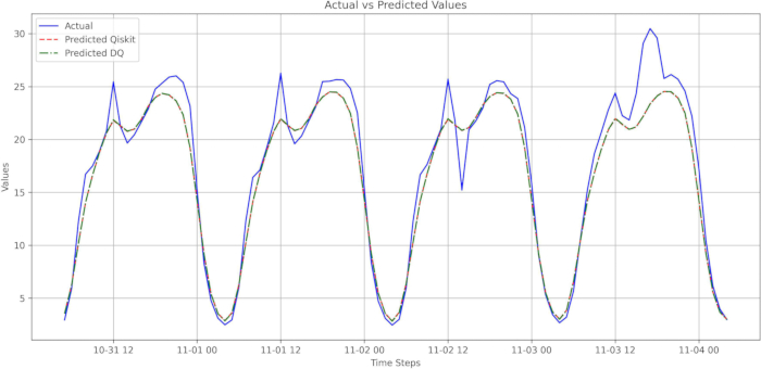
Figure 4: Comparison of prediction results of Qiskit (on quantum hardware) and DQ (on the simulator). Comparison between actual values and predictions, with predictions derived from Qiskit and DQ experiments. Please click here to view a larger version of this figure.

Table 3: Performance comparison of QTSMixer between quantum hardware and simulation experiments. Here, the MAPE and RMSE are used as the main evaluation metrics, and lower values indicate better performance. Please click here to download this Table.

Results

We conducted a detailed empirical analysis on some datasets. The first experiment is based on the LTNTF dataset. The three cities exhibited distinct data distribution patterns: City A showed a significant low point in traffic flow at the beginning of the year; City B maintained relatively high values during the same period, while City C displayed more balanced distribution throughout the year, see Supplemental Figure S1, Supplemental Figure S2,...

Discussion

In this paper, we proposed QTSMixer for long-term NTP, which is a novel quantum-classical hybrid approach with improvements in accuracy and cross-domain adaptability. This study not only expands the application potential of quantum computing in time series prediction but also points out the direction for its future deployment on real quantum hardware. However, the current quantum-classical hybrid architecture exhibits limited capability in processing exogenous variables. Future improvements could incorporate a channel-mi...

Materials

List of materials used in this article

Name	Company	Catalog Number	Comments
DeepQuantum	TuringQ Co., Ltd.	https://deepquantum.turingq.com/	An efficient programming framework for quantum machine learning and optical quantum computing developed by TuringQ.
Qiskit	IBM	https://www.ibm.com/quantum/qiskit	An open-source SDK for working with quantum computers at the level of extended quantum circuits, operators, and primitives.
ibm_brisbane	IBM	https://quantum.ibm.com/	The superconducting quantum computer in the IBM Quantum Eagle family.
LTNTF dataset	China Mobile	https://jiutian.10086.cn/open/#/dataset/710012?platform=OpenInnovation	The dataset comes from the Jiutian AI platform of China Mobile.
python3.10	Python Software Foundation	https://www.python.org/downloads/release/python-3100/
quantum re-uploading technology	Pérez-Salinas, A., Cervera-Lierta, A., Gil-Fuster, E., Latorre, J. I. Data re-uploading for a universal quantum classifier. Quantum. 4 226 (2019).	https://doi.org/10.22331/q-2020-02-06-226
BasicTS+ framework	Shao, Z. et al. Exploring progress in multivariate time series forecasting: Comprehensive benchmarking and heterogeneity analysis. IEEE Transactions on Knowledge and Data Engineering. 37 291-305 (2023).	arXiv:2310.06119v2
GPU A100	NVIDIA		80G GPU
Transformers	Hugging Face	https://huggingface.co/	The platform where the machine learning community collaborates on models, datasets, and applications.