Utilizing Whole-Cell Biosensors to Measure Ionic Mercury in Water Samples

Summary

This article presents protocols for utilizing two whole-cell biosensors (Mer-Blue and Mer-RFP) to detect ionic mercury. By providing detailed procedures for their operation and output analysis, the study aims to facilitate broader adoption and further development of these technologies for monitoring specific pollutants.

Abstract

Whole-cell biosensors (WCBs) are instrumental platforms for discovering and characterizing regulatory elements and advancing bioengineering. They also hold immense promise for environmental and food monitoring. While significant efforts have been invested in enhancing their sensitivity and portability, the standardization of their handling and data analysis remains relatively underdeveloped. This article presents a comprehensive guide to utilizing two recently developed WCBs, Mer-Blue and Mer-RFP, proven capable of detecting ionic mercury at levels below the World Health Organization's drinking water limits. The protocols detailed herein encompass microbial culture preparation, sensor calibration, data acquisition, and analysis. For the fluorometric Mer-RFP biosensor, a novel biosynthesis allocation theorem is employed to identify the time interval for reliable and accurate dose-response measurements. For the colorimetric Mer-Blue biosensor, a low-cost camera setup enables rigorous measurements in settings lacking expensive spectrophotometers and fluorimeters, facilitating decentralized pollution monitoring. The procedures used for testing freshwater samples are described, and the limitations of these biosensors with respect to sample types are discussed. By sharing these handling and analysis techniques, we encourage broader research groups to adopt and improve these biological devices for developing effective environmental monitoring solutions. Ultimately, this research aims to facilitate the widespread adoption of biosensor technologies within the environmental science community, contributing to more effective and efficient monitoring of trace element pollution in various ecosystems.

Introduction

As concerns grow over environmental pollution and the safety of the water and food supply, biosensors have emerged as an attractive, affordable alternative to traditional analytical chemistry methods. Heavy metals are highly toxic pollutants that have become increasingly prevalent due to human activities^1,2,3,4. However, conventional detection methods⁵ are often costly and inaccessible.

Mercury-sensitive WCBs harness the remarkable specificity and sensitivity of the MerR transcription factor^6,7,8. In its native function, MerR regulates the expression of effector proteins, whose detoxifying activity confers mercury resistance⁹. The ability of MerR to regulate gene expression in a mercury-dependent manner has been repurposed for the regulation of reporter proteins in mercury detection systems^{10,11,12,13,14,15,16}. Despite promising research, these WCBs have yet to be adopted for real-world monitoring. Factors such as biological fragility, specialized handling requirements, and the absence of standardized protocols and certified reference materials have hindered practical application^17,18,19,20.

A WCB system for ionic mercury detection has been developed using MerR coupled to two different reporter proteins. Mer-Blue expresses a chromogenic protein and serves as a colorimetric biosensor, enabling visual or camera-based detection. Mer-RFP, a fluorescent biosensor, allows continuous monitoring of signal accumulation. By carefully controlling the timing of sample exposure during the growth phase, robust reproducibility has been achieved in both systems¹⁵.

This article presents detailed protocols for operating both Mer-Blue and Mer-RFP, along with a comprehensive analysis of their signal outputs. For Mer-RFP, analysis is based on a recently introduced theorem of protein biosynthesis allocation²¹. For Mer-Blue, colorimetric analysis can be digitized using image processing software such as ImageJ. To ensure consistent image acquisition settings, a low-cost, DIY camera setup named PelletCam is presented. In both cases, automated software is provided to facilitate operation. By sharing accessible and standardized experimental methodologies and data analysis techniques, broader adoption of WCBs is encouraged for the development of reliable and cost-effective biosensor-based monitoring solutions.

Protocol

The reagents and the equipment used in this study are listed in the Table of Materials.

1. Preparing ionic mercury solutions

1. Weigh a small mass of HgBr₂ powder (typically between 0.1 and 0.2 g) using appropriate protective gloves and a mask to prevent inhalation and skin exposure.
2. Calculate the amount of water needed to obtain a 4 mM solution by dissolving the measured mass of solid powder in ddH₂O using the formula:
   
   NOTE: The expected volume is close to 100 mL; a simplified formula may be used:
   
   1. Alternatively, when using HgCl₂, apply the formula:
      
3. Store the stock solution in a hermetically sealed container in a refrigerated environment (4 °C) to prevent evaporation.
4. Prepare serial dilutions prior to each titration assay, starting with 1 mL of 2 mM Hg²⁺ and diluting down to 40 nM, as shown in Table 1.
   NOTE: The concentration of ionic mercury may change during storage, likely due to spontaneous reduction and evaporation of elemental mercury (Hg°). Although refrigeration and the use of high-quality, hermetic containers may reduce these effects, avoid using solutions stored for more than 6 weeks-especially for concentrations of 250 nM of Hg²⁺ or lower.

2. Preparing M9 medium

1. Dissolve reagent powders in separate flasks using ultrapure water to prepare the following stock solutions: M9 5×, 1 M MgSO₄, 1 M CaCl₂, 20% (w/v) glucose, and 20% (w/v) Casamino acids.
2. In a 500 mL or 1 L glass bottle, mix 50 mL of M9 5×, 2.5 mL of 20% (w/v) Casamino acids, and add ultrapure water to reach a total volume of 246.475 mL.
3. Autoclave the mixture and the stock solutions listed above at 121 °C for 20 min.
4. Allow all solutions to cool completely to avoid precipitation of CaCl₂.
5. Add to the cooled mixture: 25 µL of 1 M CaCl₂, 500 µL of 1 M MgSO₄, and 3 mL of 20% (w/v) glucose.
   NOTE: This results in a richly supplemented M9 medium with the following final concentrations: 0.24% (w/v) glucose, 0.2% (w/v) Casamino acids, 2 mM MgSO₄, 1 mM CaCl₂, 3 g/L KH₂PO₄, 0.5 g/L NaCl, 6.78 g/L Na₂HPO₄, 1 g/L NH₄Cl.

3. Activating the Mer-Blue / Mer-RFP biosensor

1. Use Escherichia coli DH5α cells transformed with the pUC-Mer-RFP or pUC-Mer-Blue plasmid (see Table of Materials).
2. Prepare an LB-agar Petri dish containing 100 µg/mL ampicillin.
3. Seed cells from a cryopreserved glycerol stock onto the LB-agar plate using the streaking method.
4. Incubate the plate overnight at 37 °C.
5. On the following day, pick a single colony from the LB-agar plate to inoculate a 10 mL culture using M9 medium (Figure 1A).
6. Incubate the culture at 37 °C with constant shaking at 220 rpm overnight (~16 h) (Figure 1B).

4. Titration experiment using Mer-RFP

1. Measure the optical density of the overnight bacterial culture at 600 nm (OD₆₀₀).
2. Calculate the volume of the overnight culture required to reach an OD₆₀₀ of 0.05 in a total volume of 10 mL of fresh M9 medium using the formula:
   
   where C₁ is the OD₆₀₀ of the overnight culture, and V₁ is the volume to be taken from it.
3. Centrifuge V₁ mL of the pre-inoculum at 3500 × g for 5 min. Discard the old M9 medium and resuspend the bacterial pellet in 10 mL of fresh M9 medium (Figure 1C).
4. Add 195 µL of the resuspended culture to each well of a 96-well microplate. Ensure that each micro-culture is prepared in triplicate for accurate measurements.
5. Add 5 µL of 40 nM to 40 µM ionic mercury solutions, as described in step 1, to each well to achieve final concentrations ranging from 1 nM to 1 µM (Figure 1D).
6. Place the microplate in a multimode microplate reader with temperature control, set to the following parameters (Figure 1E) - Temperature: 37 °C, Shaking: Constant shaking at 60 rpm, Time interval: Read every 15 min for 16 h, Optical density measurement: Read at 600 nm, Fluorescence measurement: Excitation at 570 nm and emission at 615 nm.
7. After completing the 16-h incubation period, collect the data from the microplate reader (Figure 1F).

5. Data analysis for Mer-RFP results

1. Use preferred spreadsheet software or data management tools to visualize raw OD₆₀₀ values over time for all individual cultures (Figure 1G). Verify that the end of the lag phase and the onset of the stationary phase occur at approximately the same time across all replicates within each mercury concentration condition. Exclude any cultures that deviate by more than 1 h from the average timing.
2. Calculate the average OD₆₀₀ for each time point across all replicates within each mercury concentration condition. For each triplicated culture condition, a single, averaged OD₆₀₀ growth curve and three fluorescent intensity outputs will be available at different time points.
3. Plot the averaged OD₆₀₀ vs. time for the culture without mercury. Visually identify and select the time interval where the growth rate is positive (see Figure 2). Exclude the remaining data points from all cultures.
4. For each culture, calculate the specific growth rate at each time point by finding the change in OD₆₀₀ from the previous time point and dividing that change by the OD₆₀₀ value at that time point, using the following formula:
   
5. Similarly, calculate the specific fluorescence production rate for each culture by finding the change in fluorescence intensity from the previous time point and dividing that change by the OD₆₀₀ value at that time point, using the formula:
   
6. For each culture, plot the specific growth rate against the fluorescence production rate (see Figure 3). Identify a linear range within the late time points. Exclude early time points until a linear regression with the highest R², based on a minimum of 12 points (approximately 3 h), is achieved.
   NOTE: The slope of this linear regression represents the expression fraction, i.e., the proportion of total protein synthesis allocated to the reporter protein²¹.
7. For all cultures, extract linear trends from approximately the same time interval and record the slope value for each condition.
   NOTE: Achieving the highest possible R² value across all cultures using the same time interval may require multiple attempts. For automated analysis, the following Jupyter Notebook (Google Colab framework) is available at https://github.com/frank-britto/Mer_RFP. This notebook serves as a template for optimizing the extraction of linear trends and further dose-response profiling.
8. Take the average slope across replicates for each mercury concentration.
9. Plot the averaged slope values against mercury concentration (see Figure 4A). Fit a Hill function to the data:
   
   Where: f_RFP is the expression fraction for Red Fluorescent Protein, H represents the maximum possible expression for the circuit, [Hg²⁺] is the ionic mercury concentration, k_Hg is related to the affinity for ionic mercury, n is the Hill coefficient that expresses the cooperativity of the response to Hg²⁺.

6. Titration experiment using Mer-Blue biosensor

1. Centrifuge an overnight, dense culture obtained as described in step 3 at 3,500 × g for 10 min.
2. Discard the spent M9 medium and resuspend the bacterial pellet in fresh M9 medium to an OD₆₀₀ of 1.0. Ensure a minimum of 5 mL of culture at this density is obtained (Figure 1C).
   NOTE: If a spectrophotometer is not available, approximate the initial conditions by resuspending the bacterial pellet in a volume of fresh M9 medium equal to twice the original volume of the dense culture.
3. Add 9.5 mL of M9 medium and 10 µL of a 100 mg/mL ampicillin stock solution to sterilized glass culture tubes (Figure 1H).
4. Inoculate the supplemented M9 medium with 500 µL of the biosensor culture prepared in step 6.2 (OD₆₀₀ = 1.0).
5. Add 10 µL of the prepared ionic mercury solutions (see step 1) to reach final concentrations of 0 nM, 1 nM, 2 nM, 5 nM, 10 nM, 25 nM, 50 nM, 100 nM, 125 nM, and 250 nM.
6. Incubate the cultures at 37 °C for 16 h with vigorous shaking at 220 rpm (Figure 1I).

7. Data acquisition and analysis for Mer-Blue results

1. Transfer approximately 1.3 mL of each culture to a 1.5 mL microtube (Figure 1J).
2. Centrifuge the microtubes at top speed for 3 min to obtain tight pellets. Discard the supernatant.
3. (Optional) To obtain larger pellets, repeat centrifugation and supernatant removal up to six times.
4. Photograph the bottom of each microtube, focusing on the pellet (Figure 1K). Use a microtube holder and a tripod or a PelletCam (see step 8) to ensure consistent and reproducible orientation, illumination, and color settings across all images (see Figure 5).
5. Determine the color intensity values of each pellet image across the red, green, and blue (RGB) channels.
   1. If using ImageJ: Load the image and navigate to Image > Type > RGB Stack to create a three-slice stack (red, green, and blue channels). Use the selection tool to draw a region of interest (ROI) around the pellet area. Navigate to Analyze > Measure to obtain the mean intensity values for the selected area in each channel.
   2. If using PelletCam: Open the .csv file containing average color intensity values for a representative nine-pixel area of the pellet image.
6. Compute the biosensor's response for each sample by calculating the Euclidean distance in RGB space relative to a white reference pellet image (non-transformed E. coli), as described previously²², using the equation:
   
   Here, R_sample, G_sample, and B_sample represent the average color intensities from each RGB channel in the selected area of the pellet image from the sample of the biosensor, while R_ref, G_ref, and B_ref denote the corresponding values for a reference pellet of non-transformed E. coli.
7. Plot the calculated Euclidean distances against the corresponding ionic mercury concentrations (see Figure 6). Fit a Hill function to the data (see Figure 4B) using the following equation:
   
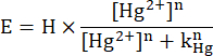
   Here, E is the Euclidean distance, H represents the maximum possible coloration for the circuit, [Hg²⁺] is the ionic mercury concentration, k_Hg is related to the affinity for ionic mercury, and n is the Hill coefficient that expresses the cooperativity of the response to Hg²⁺.

8. Building a PelletCam

1. Download the files to build a closed microcontroller system for color measurement in bacterial pellets from the website (https://github.com/EhbAIGit/PelletCam-OPENBIOLAB-AI).
   NOTE: Basic knowledge of laser cutting, 3D printing, ESP32, and Arduino is helpful. An introductory guide to ESP32-CAM is available at (https://lastminuteengineers.com/getting-started-with-esp32-cam/?utm_content=cmp-true). It is recommended to purchase the ESP32-CAM together with the MB Adapter for easier programming. For users unfamiliar with the ESP32, it is recommended to follow the tutorial at https://lastminuteengineers.com/esp32-arduino-ide-tutorial/ first.
2. Use the LasercutterBox.ai file to cut and engrave a 3 mm multiplex with a laser cutter.
3. Build the parts from file ESP32SET.stl file with a 3D printer. This .stl file can be imported directly by almost all 3D printer software; for example, Bambu studio (https://bambulab.com/en/download/studio).
4. Install the ESP32 (ESP32-CAM-MB 2640 WiFi Bluetooth-camera module) by placing the .cpp and .h and .ino files in a single folder. Next, open the .ino file with Arduino IDE software and click on >Upload. Once uploaded, the ESP32 will start automatically.
5. At this point, the user should be able to connect to the WiFi access point named >PELLET and password >PELLETCAM, as specified in the .ino file of the ESP32. The IP address of the PelletCam will be displayed in the Arduino IDE’s serial monitor. Open a web browser and navigate to the address: http://192.168.4.1.
   NOTE: This will enable to view the image or to take a new image (>CAPTURE PHOTO), rotate the image (>ROTATE), or set the luminance of the LED strip (>LEDS).
6. Connect the ESP32 Arduino to the LED strip (NeoPixel Stick - 8 x 5050 RGB LED with Integrated Drivers) and a 5V USB cable according to the scheme in the file InstallationManual.pptx.
7. Use a glue gun to glue the ESP32 and LED strip to the 3D-printed supports.
8. Insert a microtube with a colored bottom (or a bacterial pellet) in the 3D-printed front of the PelletCam. Position the ESP32-LED-support approximately 5 cm further and take a picture via the webpage. If a sharp and properly illuminated image is obtained, then glue the ESP32-LED-support on the bottom of the wooden box. If not, adjust the distance between the front and the ESP32-LED-support and repeat the procedure until a satisfying distance is obtained.
9. Assemble the box by using masking tape and gluing all parts together with wood glue.
10. Connect the PelletCam via the USB cable to a USB power supply that can deliver at least 1 A.
    NOTE: Ensure to have Python 3.9 or a later version installed.
11. Open a command prompt or terminal window. Navigate to the directory containing the pellet.py file. Execute the script using the command >python pellet.py.
12. If the pellet.py script cannot run, it might be due to missing Python libraries. Install the required libraries using the command >pip install pillow tkinter pathlib statistics. For extra guidance to set up your own system, refer to the document PelletCam Example.docx.

9. Measuring environmental water samples

1. Collect samples from environmental sources such as rivers or ponds and store them in airtight containers at low temperatures to minimize evaporation. For details, see the Discussion section.
2. Centrifuge the samples at 3,500 × g for 10 min to sediment sand and organic debris, isolating the aqueous fraction.
3. Sterilize the clarified sample using a 0.22 µm syringe filter.
   NOTE: Avoid heat sterilization, as mercury is volatile and may evaporate during the process.
4. (Optional) Prepare a separate acidified aliquot by adding 5% HCl for independent measurement using standard analytical chemistry techniques. Use only the non-acidified sample for biosensor assays.
5. Mix 5 mL of the sterile-filtered environmental sample with 4.5 mL of 2× M9 medium, resulting in a 1:2 dilution of the sample.
6. Inoculate the diluted sample-medium mixture with 0.5 mL of an overnight culture (prepared as described in step 5.4). This inoculation corresponds to a 20-fold dilution of the culture, yielding an OD₆₀₀ of 0.05 to initiate the assay.
   1. If using Mer-RFPTransfer 200 µL of the sample-medium mixture to a microplate well and initiate measurements using a microplate reader as described in step 3.6.
   2. If using Mer-Blue: Incubate the 10 mL sample-medium mixture at 37 °C for 16 h with vigorous shaking at 220 rpm, as described in step 5.6.

Results

Both biosensors exhibit no detectable baseline expression of their respective reporter proteins under mercury-free conditions. Mer-Blue cultures typically begin to display visible coloration to the naked eye between 6-8 h post-inoculation at HgBr₂ concentrations of 25 nM and above. When properly conducted, titration experiments using either Mer-RFP or Mer-Blue yield responses that fit a Hill function with a Hill coefficient close to 1, indicating non-cooperative binding behavior²³.

...

Discussion

The biosensor circuits utilized here are identical, only differing in the reporter protein. Both are entirely encoded on high-copy plasmids, enabling their deployment in Escherichia coli cells of various strains. While functional in E. coli B strain cells, a stronger colored signal from Mer-Blue was observed in K-12 strains, specifically DH5α and chemically competent E. coli cells¹⁵.

We observed that achieving a reliable output requires a subs...

Materials

List of materials used in this article

Name	Company	Catalog Number	Comments
3 mm thick multiplex wood	Many distributors
5 V USB cable	Many distributors
96-well Clear Flat Bottom Polystyrene TC-treated Microplates	Corning	3599
Agar powder	HiMedia	GRM026
Ampicillin	Gold Biotechnology, Inc.	A-301-100
CaCl2	Millipore	208290
Casamino Acids	Calbiochem	2040OP
D-(+)-Glucose	Central Drug House (P) Ltd.	506250
ESP32-CAM-MB 2640 Bluetooth WiFi Camera Module USB to Serial Port Development Board Auto Download (Type C)	Many distributors
Glass culture tubes	Corning	9825
HgBr2, Mercury(II) bromide	Merck	200085
HgCl2, Mercury(II) chloride	Merck	21465
Luria broth (Miller)	Sigma-Aldrich	L3522
M9 minimum salts	Sigma-Aldrich	M6030
MgSO4	HiMedia	GRM684
NeoPixel Stick - 8 x 5050 RGB LED with Integrated Drivers	Adafruit	1426
Plasmid: pUC-Mer-Blue	Our group	-	Full sequence available in https://www.mdpi.com/article/10.3390/bios14050246/s1
Plasmid: pUC-Mer-RFP	Our group	-	Full sequence available in https://www.mdpi.com/article/10.3390/bios14050246/s1
Syringe filters, hydrophilic, pore size 0.22 microns	Millipore	SLGV004SL	For sterilizing environmental samples.