Dual Encoder-Decoder-Encoder with Adversarial Training for Unsupervised Traffic Accident Detection in Surveillance Videos

Summary

This work proposes a dual encoder-decoder-encoder (EDE) model for automated traffic accident detection. Using a two-phase training method, it learns normal driving patterns and identifies anomalies via generative confrontation. The model effectively detects accidents in real-world footage and offers insights into driver behaviors by capturing subtle deviations.

Abstract

To enhance road safety and improve emergency response, traffic incidents should be detected in real-world surveillance footage as quickly as possible. Existing systems largely depend on manual monitoring, which is time-consuming and prone to error. Automated accident detection remains challenging due to the substantial class imbalance: normal driving situations are overrepresented, whereas accidents are rare and diverse. In such cases, traditional computer vision systems often cannot reliably differentiate between normal and abnormal events. This study addresses the problem by developing a deep learning architecture based on a dual encoder-decoder-encoder (EDE) framework. The model uses two shared encoder-decoder pipelines to map image distributions to specified latent distributions in both directions. This framework enables the system to model common traffic behavior patterns and become more sensitive to changes that may indicate dangerous or unusual events. A two-phase training technique is proposed to further improve anomaly detection. In the first phase, the model learns to reconstruct images of normal driving, using reconstruction loss to characterize normal behavior. In the second phase, a generative adversarial mechanism is introduced: reconstructed latent vectors from one EDE are passed to the other, generating synthetic images and latent spaces. This process amplifies differences between real and synthetic outputs, making the system more responsive to subtle signs of potential anomalies. The dual-EDE architecture and adversarial training methodology represent a substantial advance over current methods by modeling both normal and pathological behavior. Experimental results on real-world traffic surveillance datasets demonstrate that the proposed method significantly improves the detection of accidents and unsafe driving behaviors, both in terms of accuracy and robustness.

Introduction

According to the World Health Organization (2023), road traffic injuries are the leading cause of death among children and young adults aged 5-29 years, with approximately 1.3 million fatalities reported globally each year. This alarming statistic underscores the urgent need for automated systems capable of monitoring road traffic¹, detecting anomalies in real time, and reducing delays in emergency response. The integration of artificial intelligence (AI) and the Internet of Things (IoT) into smart city infrastructure has enabled the development of intelligent transportation systems. While closed-circuit television (CCTV)^2,3 networks provide continuous surveillance of urban traffic, manual monitoring is impractical and prone to error. Therefore, scalable, automated solutions for traffic incident detection are essential.

Traditional computer vision methods for traffic analysis -- such as vehicle detection, tracking, and behavior classification -- often employ convolutional neural networks (CNNs) trained via supervised learning^4,5. These systems require extensive annotated datasets and often fail to generalize across the rare and varied scenarios that characterize real-world accidents. Consequently, researchers have turned to unsupervised anomaly detection approaches, which do not depend on labeled anomaly data. Among these, autoencoders (AEs) and generative adversarial networks (GANs) have shown promise in modeling normal patterns and identifying deviations^6,7,8.

However, standard AEs tend to reconstruct inputs too faithfully -- even when those inputs are anomalous -- leading to high false-negative rates^9,10. Variational autoencoders (VAEs)¹¹ and GAN-based models such as f-AnoGAN¹², GANomaly¹³, and OCGAN¹⁴ address some of these issues by incorporating latent-space modeling and adversarial learning. Nonetheless, these models often rely on unidirectional mappings from image to latent space¹⁵, limiting their ability to detect subtle or complex inconsistencies in real-world traffic anomalies.

Supervised systems, such as those developed for the AI City Challenge by ByteDance¹⁶, WHU¹⁷, and USF¹⁸-achieve high accuracy through spatiotemporal tracking¹⁹and object-centric designs. However, they require labeled accident data and complex tracking pipelines, reducing scalability and applicability in real time.

Model	Type	Key Features	Limitations	Performance (Described)
GANomaly	Unsupervised	Encoder–Decoder–Encoder; adversarial training	Tends to reconstruct even anomalous inputs too well, leading to false negatives	Good overall, with high precision and balanced recall
OCGAN	Unsupervised	One-class GAN with constrained latent space	Struggles with detecting subtle or complex anomalies	Slightly better than GANomaly, with improved balance across metrics
f-AnoGAN	Unsupervised	Fast anomaly detection using GANs and feature matching	Limited ability to capture complex anomalies in latent space	Moderate performance (specific scores not provided)
ByteDance	Supervised	Spatiotemporal tracking with object-level anomaly localization	Requires labeled training data; limited scalability in real-world settings	Very high accuracy and precision; slightly lower sensitivity
BADU	Supervised	Uses background modeling and vehicle tracking	Less effective in diverse scenes; misses subtle anomalies	Solid accuracy; good balance but lower than top methods
WHU	Supervised	Dual-modality trajectory tracing	Poor generalization and low anomaly recall	Weak performance overall, especially in detecting anomalies
USF	Supervised	Combines background modeling with structural similarity analysis	Poor at identifying anomalies accurately	Very low accuracy and sensitivity
Proposed (Dual-EDE)	Unsupervised	Dual encoder–decoder–encoder; bidirectional latent mapping with adversarial and contrastive loss	High computational load; limited to RGB input	Excellent performance; top precision, high recall, and strong balance across metrics

Table 1: Summary of related work in video-based traffic anomaly detection.

Table 1 contrasts essential anomaly detection methods used in traffic surveillance, highlighting their architectures, advantages, drawbacks, and performance. Conventional GAN-based models like GANomaly and OCGAN can perform effective unsupervised detection but struggle with subtle abnormalities. Supervised methods, while highly accurate, depend heavily on labeled data and sophisticated tracking. The proposed Dual-EDE model integrates bidirectional latent space encoding with adversarial and contrastive training, enabling it to detect rare and subtle traffic anomalies without labeled data, offering both scalability and robustness.

Research gap and hypothesis
Although unsupervised models mitigate the need for labeled anomalies, they still struggle with accurately detecting rare, subtle, and high-impact traffic events. Current methods are limited by architectural asymmetry and the inability to fully exploit latent-space inconsistencies. Many also fail to robustly distinguish between complex normal behavior and genuine anomalies in highly dynamic traffic environments.

We hypothesize that a dual encoder-decoder-encoder (EDE) architecture trained exclusively on normal traffic data, combined with a two-phase training strategy, can outperform state-of-the-art models in detecting diverse and subtle traffic anomalies. By enforcing bidirectional latent consistency and integrating adversarial reconstruction, the system becomes more sensitive to minute deviations from expected behavior -- such as sudden braking, erratic swerving, or collisions -- without the need for annotated accident data.

Proposed method
We propose a novel unsupervised anomaly detection framework built upon a dual-EDE architecture. Unlike traditional models that employ a single encoding-decoding pipeline, our system uses two EDE pathways that perform bidirectional mapping between images and latent representations. This design enables the model to learn rich features of normal traffic dynamics and to amplify discrepancies when anomalies occur. The training process consists of two phases:

Phase One uses reconstruction loss to model normal behavior, akin to standard autoencoder training.

Phase Two introduces a generative adversarial mechanism, where latent vectors from one EDE are passed into the second to generate synthetic data, forcing the system to maximize distinctions between real and fake representations in both image and latent domains.

Key contributions
We introduce a dual-EDE architecture that captures latent inconsistencies through bidirectional mapping for improved anomaly detection. We develop a two-phase training procedure that combines autoencoder reconstruction with adversarial learning to enhance sensitivity to subtle deviations. We demonstrate, through experiments on the AI City Challenge (Track 4) dataset, that the model outperforms several state-of-the-art supervised and unsupervised baselines, achieving robust and scalable accident detection in real-world urban environments. In summary, this work offers a scalable, accurate, and label-free approach to traffic anomaly detection, contributing to safer and more responsive smart transportation systems.

Protocol

System

Setup
We deployed the proposed traffic anomaly detection system within a hierarchical and distributed computing framework, leveraging the Intel Tiber Cloud environment. This architecture comprises three tiers -- edge, fog, and cloud -- to ensure low-latency inference, scalable training, and efficient resource allocation across compute nodes.

Edge Tier: Real-time anomaly detection is conducted at the edge using lightweight, GPU-capable embedded devices (e.g., NVIDIA Jetson Nano or equivalent Intel-based platforms with integrated GPUs). These units were co-located with surveillance cameras and executed frame-by-frame inference with minimal latency, enabling decentralized and responsive traffic monitoring.

Fog Tier: More compute-intensive tasks, including batch inference and real-time model refinement, were handled by fog nodes provisioned as dedicated virtual machines or bare-metal instances within the Intel Tiber Cloud. Each fog node was configured with an Intel Xeon processor with at least 16 GB of RAM and had access to Intel-integrated or discrete GPU acceleration. This intermediate layer enabled high-throughput operations near the data source while maintaining autonomy from central servers.

Cloud Tier: For large-scale training and archival, the cloud tier utilizes scalable compute clusters offered through Intel Tiber's AI-optimized services. Instances equipped with Intel Habana Gaudi accelerators or Intel Xeon Scalable processors are employed for training deep neural networks on extensive video datasets, supporting model versioning, long-term storage, and system-wide orchestration.

The full software stack operated in a Python 3.8+ environment using Intel-optimized libraries for accelerated computation. The primary frameworks include PyTorch (with Intel Extension for PyTorch), OpenCV for image and video preprocessing, and Scikit-learn for evaluation. GPU acceleration is enabled through the appropriate oneAPI toolkits and DAAL optimizations.

Upon deployment, we cloned the repository containing the dual-EDE architecture and initialized the model components -- two encoders (E1, E2) and two decoders (D1, D2). Employed the .to(device) method to transfer the components dynamically to the optimal processing unit (CPU, GPU, or Gaudi accelerator) depending on local resource availability.

We declared the training and evaluation parameters, including the number of epochs, learning rate, loss-balancing coefficients (γ, δ), and anomaly sensitivity thresholds (ω₁, ω₂), in a configuration script. For training, we followed a two-phase protocol: (1) standard autoencoder reconstruction for learning normal traffic behavior and (2) adversarial latent reconstruction to amplify anomalies using cross-EDE interactions.

This modular and cloud-native system architecture enabled robust, real-time anomaly detection, model scalability, and reliable deployment in real-world intelligent transportation environments via the Intel Tiber Cloud.

Dataset
For training and evaluating the proposed anomaly detection system, we used the dataset provided by the NVIDIA AI City Challenge 2021, Track 4 (Traffic Anomaly). The dataset comprises 100 training videos and 150 testing videos, each averaging 15 min in duration, recorded at 30 fps and 410 p resolution. Each video presents a distinct level of difficulty due to variations in road types, camera angles, lighting, and weather conditions. The dataset captures a wide range of road infrastructure (e.g., multi-lane highways, intersections), traffic densities, and weather conditions (e.g., clear, rainy, dusk), from multiple camera angles. These attributes make it an ideal benchmark for evaluating the generalizability of anomaly detection models.

Preprocessing
To train the model under unsupervised conditions, use only normal (non-accident) traffic scenes, avoiding any exposure to anomalous events during training. Perform video preprocessing using OpenCV. Sample frames uniformly at 5 fps to ensure sufficient temporal coverage while reducing redundancy. Resize frames to 128 x 128 pixels, matching the input requirements of the dual-EDE network and balancing visual detail with computational efficiency. Normalize pixel values to the range [−1, 1] to improve training stability.

To improve generalization and simulate real-world variability, apply the following augmentation techniques to each training frame with randomized probability:

Random cropping and scaling: Crop random subregions and scale them back to the original resolution, encouraging invariance to object size, partial visibility, and spatial position shifts, mimicking zoom effects and off-center subjects in surveillance video.

Brightness and contrast modulation: Apply linear or gamma-based transformations to mimic lighting variations such as shadows, glare, sunrise/sunset variations, and artificial illumination. This improves the model's resilience to diurnal and seasonal lighting fluctuations.

Gaussian noise injection and motion blur: Add Gaussian noise with varying standard deviations to simulate sensor noise and compression artifacts. Simulate motion blur using convolutional kernels oriented in different directions and magnitudes to emulate the effect of moving objects or camera shake, which is particularly relevant in fast-paced traffic scenes.

Random occlusion masking: Apply synthetic occlusions by superimposing black or gray rectangular patches of random sizes and locations over the frame. This augmentation simulates real-world obstructions such as pedestrians, infrastructure elements, or passing vehicles occluding the field of view. It encourages the model to learn from context and remain robust to missing or distorted regions.

Apply these augmentations dynamically during training using PyTorch transformation pipelines, ensuring each batch contains a diverse mix of augmented frames, promoting exposure to diverse patterns and reducing overfitting.

Load processed frames with PyTorch's DataLoader to manage batching, shuffling, and parallel loading. Train with batch sizes between 32 and 64, depending on GPU capacity. For inference and anomaly scoring, process frames individually (batch size = 1) to enable precise frame-level detection.

This preprocessing and augmentation pipeline improves robustness and generalization, allowing the model to detect anomalous behavior effectively in diverse and noisy real-world traffic monitoring environments.

The proposed method:
The proposed EDE system learns bidirectional mappings between image distributions and latent spaces. Two encoders and two decoders enable robust feature extraction and anomaly differentiation. The networks are trained in both reconstruction and adversarial stages. Contrastive learning, regularization, and gradient penalty are used to prevent mode collapse and improve GAN training robustness.

The EDE framework operates as follows: Encoder 1 (E1) encodes image features into the latent space. The first decoder (D1) reconstructs images from latent vectors to minimize reconstruction loss. The reconstructed images are then mapped back into the latent space to capture inconsistencies. The second decoder (D2) generates synthetic images from the second latent space to help the model distinguish real from synthetic data. This bidirectional mapping detects anomalies based on latent space discrepancies rather than pixel-level differences.

Phase 1: Reconstruction Training: The autoencoder is trained to reconstruct normal traffic images, so anomalous inputs produce substantial reconstruction errors. The loss function considers the input image, its latent encoding, and the reconstructed image.

Adversarial Training: Following reconstruction training, adversarial learning is applied. Reconstructed latent vectors are passed through an alternate EDE structure to produce synthetic images and latent vectors. The goals are to maximize differences between real and synthetic images; alter and reconstruct latent vectors to enhance anomaly detection by Encoder 2 (E2); and prevent encoder collapse.

Training is designed to avoid convergence of E1 and E2 to identical mappings, which would reduce discriminative capability.

Contrastive learning: A loss function differentiates real and reconstructed representations, with a margin hyperparameter controlling the separation of features.
Regularization techniques include:

Dropout: Random deactivation of neurons to prevent overfitting.
Weight decay: Penalizes large weights to stabilize feature learning.

Adversarial training stability²⁰ and mode collapse prevention methods include:
Gradient penalty: Regulates discriminator behavior.
Data augmentation: Random cropping, scaling, and adjustable lighting to simulate varied conditions.
Noise injection: Adding realistic noise, motion blur, and occlusions to improve generalization.
Early stopping: Halting training if validation loss fluctuates significantly to avoid overfitting.

These architectural enhancements, training methods, and resilience measures ensure reliable traffic anomaly detection.

The unsupervised accident detection network is trained exclusively on normal samples and tested on both normal and accident samples. Formally:

From the set of all normal and accident videos, consider a large training dataset E with only F normal frames (E = {x1, x2}). .., xM } and a smaller testing dataset Ê containing both normal and accident photographs (Ê=[( x̂1,y1), (x̂2,y2), (x̂F*,yF*)]),frames, where yi [0, 1] is the frame label image. For F F* training, the training dataset must be significantly larger than the testing dataset. After learning the dataset manifold (E), identify accident frames in Ê as outliers during inference. The model f computes an accident score Acc(x) based on the learned normal data distribution. A test image x with a high accident score may be an accident. Judgment criteria are based on the accident score threshold (φ) if Acc(x) > φ.

Network architecture:
As shown in Figure 1, the GANomaly model²¹ contains two encoders, one decoder, and one discriminator. Many researchers have adapted this method to distinguish latent vectors and detect visual anomalies^12,22. The two encoders and single decoder reciprocally modify the picture and latent vector in the model. These aberrant facts are indicated during transformation. The discriminator divides the generated images from the original. GANomaly relies on encoding, decoding, and re-encoding.

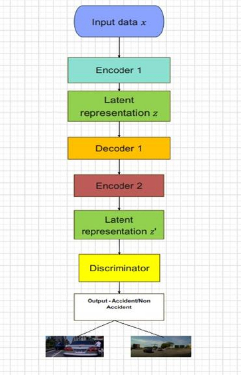
Figure 1: GANomaly architecture demonstrating the flow of information. The architecture consists of an encoder-decoder-encoder framework integrated within a generative adversarial network. The first encoder compresses the input video frame into a latent space representation, which is then reconstructed by the decoder. A second encoder maps the reconstructed frame back into the latent space. The discriminator evaluates the difference between the input and reconstructed features to compute the anomaly score. Arrows indicate the directional flow of data through the network. Abbreviation: GAN = generative adversarial network. Please click here to view a larger version of this figure.

Figure 2 illustrates the EDE architecture with two encoders and one decoder. The EDE structure must constantly change parameters to detect video mishaps. We added a second decoder to the EDE structure and let them share the encoders to generate the model in Figure 2 with two network configurations. Two encoders have four convolutional layers. We used LeakyReLU activation functions for all layers except the output layer, which used a tanh activation to bound the outputs between -1 and 1. Batch normalization was applied after multiple convolutional layers. The decoders (Figure 3 and Figure 4) are similar to the encoders but employ ConvTranspose and extra batch normalization instead of each layer.

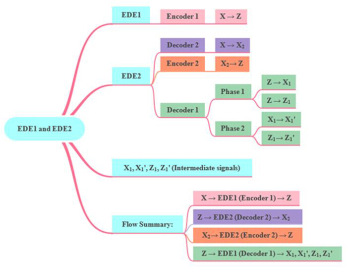
Figure 2: Proposed EDE-based architecture with information flow. The EDE architecture is illustrated, showing the flow of video frames through two encoders and a decoder. The first encoder (E1) compresses the input frame into a latent representation, which is then reconstructed by the decoder (D1). The reconstructed output is passed through the second encoder (E2) to obtain a second latent vector. Discrepancies between latent vectors and reconstruction quality are used for anomaly detection, supported by adversarial and contrastive loss components. Abbreviation: EDE = encoder-decoder-encoder. Please click here to view a larger version of this figure.

Network architecture details:
The dual-EDE model consists of two encoder-decoder-encoder pipelines, each with the same structure and jointly optimized during training.

Encoder Architecture (E1, E2)

Input: 128×128×3 RGB frame

Layer 1: Conv2D (64 filters, 4×4 kernel, stride 2, padding 1) → LeakyReLU (α = 0.2)

Layer 2: Conv2D (128 filters, 4×4, stride 2, padding 1) → BatchNorm → LeakyReLU

Layer 3: Conv2D (256 filters, 4×4, stride 2, padding 1) → BatchNorm → LeakyReLU

Layer 4: Conv2D (512 filters, 4×4, stride 2, padding 1) → BatchNorm → LeakyReLU

Layer 5: Flatten → Dense to latent vector (z ^100)

Decoder Architecture (D1, D2)

Input: z ^100 → Dense → reshape to 8×8×512

Layer 1: TransposedConv2D (256 filters, 4×4, stride 2, padding 1) → BatchNorm → ReLU

Layer 2: TransposedConv2D (128 filters, 4×4, stride 2, padding 1) → BatchNorm → ReLU

Layer 3: TransposedConv2D (64 filters, 4×4, stride 2, padding 1) → BatchNorm → ReLU

Layer 4: TransposedConv2D (3 filters, 4×4, stride 2, padding 1) → Tanh

The reconstructed image is re-encoded through the second encoder to obtain a latent representation, and discrepancies between the original and reconstructed latent vectors are used for anomaly scoring.

Activation and normalization
Encoders use LeakyReLU activation and batch normalization.Decoders use ReLU activation, except for the final layer, which applies Tanh to normalize outputs to the range [−1, 1].

Loss Functions
Image reconstruction loss: ǀǀ x −ǀǀ₂
Latent consistency loss: ǀǀ z −ǀǀ₂

Adversarial loss: Introduced in Phase II to maximize divergence between real and synthetic reconstructions by forcing the network to distinguish real latent codes from those generated during reconstruction.

This architecture captures both pixel-space and latent-space irregularities, enabling detection of subtle deviations indicative of abnormal driving behavior.

Training in two phases
A two-stage network training method is employed. For both image and latent vector reconstruction, two EDE structures are trained. In the second phase, Encoder 2 attempts to deceive Encoder 1 into misclassifying data as real or reconstructed.

Initial reconstruction training
The EDE structure is trained to replicate the input image and latent vector. Input x is encoded into latent vector z by Encoder E1. Both D1 and D2 decode z to produce images, x1 and x2. We obtained two latent vectors (z1 and z2) from encoder E2 after passing two reconstructed pictures (x1 and x2). This stage contains these training objectives:

LEDE1 = γ ǀǀ x −x₁ǀǀ₂+δ ǀǀ z −z₁ǀǀ₂   (1)
LEDE2 = γ ǀǀ x−x₂ǀǀ₂+δ ǀǀ z −z₂ǀǀ₂    (2)

These reconstructed images are passed through Encoder E2 to obtain latent vectors z₁ and  z₂. Training objectives:
Weighting factors (γ, δ) crucially influence the impact of loss components on the objective function.

Second, we trained two Encoder-Decoder-Encoder structures using adversarial methods.
Here, γ and δ are the parameters that weigh the contributions of reconstruction and latent consistency losses.

Adversarial training
Two EDE structures are trained adversarially. learns to recognize encoder 2 from data. EDE2 must deceive EDE1 because it is the opposite. D1 decodes z2 from the first step and reconstructs x1'. Repeating x1' to encoder E2 yields z1'. The stage training objectives are as follows:

min max γ ǀǀ x −x₁'ǀǀ +δ ǀǀ z -z₁'ǀǀ₂   (3)
EDE2 EDE1

The two EDE structures have these loss functions:
LEDE1 = −γ ǀǀ x -x₁'ǀǀ₂ −δǀǀ z - z₁'ǀǀ₂   (4)
LEDE2 = +γ ǀǀ x - x₁'ǀǀ₂+δ ǀǀ z - z₁'ǀǀ₂   (5)

The values of γ and δ match the previously specified parameters.

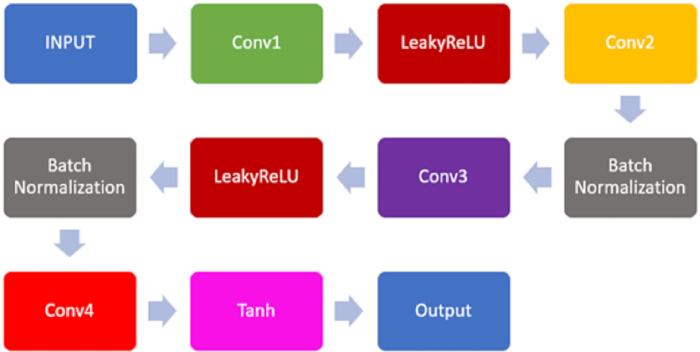
Figure 3: Encoder structure. The encoder network used in the proposed EDE architecture extracts spatiotemporal features from the input video frames. It consists of multiple convolutional layers followed by batch normalization and ReLU activation, progressively reducing spatial dimensions while capturing hierarchical representations. The final latent vector encodes high-level semantic information essential for anomaly detection. Abbreviations: ReLU = Rectified Linear Unit, EDE = encoder-decoder-encoder. Please click here to view a larger version of this figure.

Each EDE provides two loss functions for the proposed structure. In Phase 1, EDE1 must reduce x and z reconstruction losses. EDE1 must optimize phase 2 variance between latent vectors z and z1' and x and x1'. EDE2 and EDE1 reduce phase 1 x and z reconstruction errors. EDE1 must decrease the difference between z and z1' and x and x1' in phase 2, but the opposite must happen.

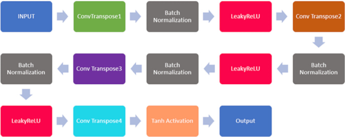
Figure 4: Decoder structure. The decoder component of the proposed EDE architecture reconstructs input frames from latent features. It consists of a series of transposed convolutional layers that progressively upsample feature maps to the original frame resolution. The decoder learns to accurately reconstruct normal traffic scenes, enabling the system to identify anomalies based on reconstruction errors. Abbreviation: EDE = encoder-decoder-encoder. Please click here to view a larger version of this figure.

Each EDE model dual training objective includes loss functions with weights that change over time:

L_EDE1=(γ||x−x₁||₂+δ||z−z₁||₂)−(1−)(γ||x−x₁''||₂+δ||z−z₁''||₂)    (6)
L_EDE2=(γ||x−x₁||₂+δ||z−z₁||₂)+(1−)(γ||x−x₁''||₂+δ||z−z₁''||₂)    (7)

The training period count is n.

Algorithm 1 shows the two-phase training:
Input:
     All normal images in Dataset E = {x₁, x₂, . . . , x_F},
          Epochs N,
     Weighted parameters γ, δ
     Output:
     Trained Encoder-Decoder-Encoder 1,
           Encoder-Decoder-Encoder 2
e₁, e₂, d₁, d₂ ←initializing
weights
n ←1
repeat
for f = 1 to F do
     z_f←e₁(x_f)
         ←d₁(z_f)
         ←d₂(z_f)
         ←e₂()
         ←e₂()
         ←d₁()
         ←e₂()′
L_EDE1←(γ||x_f−||₂+δ||z_f−||₂) −(1−)(γ||x_f−'||₂+ δ||z_f−'||₂)
L_EDE2←(γ||x_f−||₂+δ||z_f−||₂) +(1−) (γ||x_f−'||₂+ δ||z_f−'||₂)
  e₁, e₂, d₁, d₂←update weights
     using L_EDE1and L_EDE2
     end for
n ←n + 1
    until n = N

Training phases and anomaly detection criteria
Divide the training into two sequential phases:

Phase I - Reconstruction Learning:
Both EDE pipelines are trained solely on normal traffic scenes.

Input images are passed through Encoder 1 → Decoder 1 → Encoder 2 (Figure 5).

The model minimizes image reconstruction loss and latent consistency loss. This phase allows the network to learn a compact, consistent latent space for normal behavior.

Phase II - Generative Confrontation Learning:

Latent vectors reconstructed from Decoder 1 are input to Decoder 2 and then re-encoded via Encoder 1. This circular flow helps the model detect inconsistencies in synthetic patterns. An adversarial loss is added to exaggerate small deviations between original and reconstructed representations. A discriminator is optionally trained to differentiate real latent codes from reconstructed ones, enforcing sharper distinction in the latent space.

Anomaly detection:
At inference time, pass a test frame through the dual-EDE pipeline. Compute three metrics: pixel-wise reconstruction error, latent vector discrepancy, and adversarial discriminator score (if used). Calculate a composite anomaly score as a weighted sum:

Frames with anomaly scores above a calibrated threshold are flagged as potential abnormal events. This mechanism enables the model to detect subtle deviations in visual and latent space patterns without requiring any annotated anomaly labels.

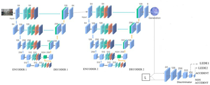
Figure 5: Architecture of the adversarial GANomaly model integrating EDE 1 and EDE 2. This figure illustrates the design of the adversarial anomaly detection model, which integrates two EDE structures-EDE1 for reconstruction and EDE2 for latent feature alignment. The model employs a latent vector consistency loss and adversarial training via a discriminator to enforce similarity between the latent representations of the input and reconstructed frames. This architecture enhances anomaly detection by learning robust feature embeddings for normal traffic patterns. Abbreviations: EDE1 = First encoder-decoder-encoder structure for reconstruction; EDE2 = Second encoder-decoder-encoder structure for latent feature alignment. Please click here to view a larger version of this figure.

During detection, our model employed these anomalous scores:

Acc(x̂) = ω₁||z−z₂||₂+ω₂||z−z₁'||₂    (8)

Changing weight parameters (ω₁+ ω₂= 1) can change sensitivity by adjusting the true positives to false positives ratio. In real-world applications, changing these two parameters can detect accidents with varied sensitivities in one experiment.

During training, each input frame x is passed through Encoder E₁ to generate a latent vector z. The latent vector is then reconstructed via Decoder D₁, producing image x̂₁, which is subsequently passed through Encoder E₂ to obtain a reconstructed latent vector z. In parallel, z is decoded by Decoder D₂ to produce x̂₂, which is also re-encoded via E₂ to yield z₂. This bidirectional process preserves both pixel- and latent-level information for anomaly detection.

Model testing algorithm:
={( x̂₁,y₁),( x̂₂,y₂),…,( x̂_M*,y_M*)},
Threshold ϕ,

Weighting parameters ω₁, ω₂
Output: Prediction label of testing dataset
E_re = {y_1pre, y_2pre, …, y_F*pre}
for i =1to F* do
z_i ← e₁(x_i)
x_2i ← d₂(z_i)
z_2i ← e₂(x_2i)
z_1i' ← d₁(z_2i)
z_1i' ← e₂(z_1i')
Acc(x̂_i) ←ω₁||z_i−z_2i||₂+ω₂||z_i−z_1i'||₂
ifAcc(x̂_i) ≥ϕ then
y_ipre ←1
else
y_ipre ←0
endif
end

EDE uses the discriminator as an adversarial learning component to increase anomaly detection accuracy by improving the model's ability to distinguish normal and abnormal events. It boosts performance as follows:

Learning discrimination: The discriminator is trained to differentiate synthetic and dual EDE structure-reconstructed representations. Optimizing this adversarial process gives the model highly discriminative latent features, improving traffic scene anomaly detection.

Removing bad reconstructions: Because they deviate so much from traffic patterns, anomalies often generate reconstruction issues. The discriminator penalizes incorrectly reconstructed frames, improving the network's normal/abnormal event detection.

Enhancing feature representation with adversarial training: By integrating adversarial learning, the discriminator makes the EDE network generate more durable and meaningful latent embeddings. This detects even little changes like abrupt braking, collisions, and vehicle swerving, improving anomaly detection.

Removing false positives: Traditional autoencoders overgeneralize and normalize anomalies, resulting in high false-positive rates. The discriminator preserves anomalies' attributes during reconstruction by identifying latent discrepancies between normal and anomalous frames.

Improving classification with two-stage decision process: Normal or abnormal rebuilt frames receive confidence scores from the discriminator. Misclassification errors and reconstruction loss are reduced in this additional verification phase, improving detection accuracy.

We used proven accident detection methods to test the strategy^23,24,25,26. One class in a multi-class dataset was normal and all others accident classes were carefully examined using one versus all approaches. The model was trained using just normal class data, whereas the test set used accident and normal data. Training and test sets were divided in two ways.

We trained and tested with 80% and 20% normal-class data, respectively. The accident class test results were randomly picked. The evaluation was unbiased by employing accident class test samples, which represent 20% of normal-class data, to avoid model skewing towards the majority normal class. The model can be tested against equal numbers of normal and accident data, representing practical conditions. It tests model generalization impartially by training with 80% of normal data and hiding 20%. This also shows that normal occurrences outnumber accidents in real life, making it important to expose the model to infrequent accident data. Randomly selecting accident samples and testing the model against all accident situations without overfitting increase robustness. The 80/20 data split is common in machine learning. Training data for meaningful patterns and test data for performance evaluation are balanced.

The experiments used datasets for training and testing. Normal-class training split was used for validation and training. All classes' test data were tested.

Model pruning and quantization greatly reduce model size and computation. The reduced model has the same accuracy but lower performance as it comprises 40% fewer parameters. For edge devices with low processing power, quantizing the model compresses it. This optimization meets real-time traffic surveillance precision and recall needs.

Lightweight designs such as MobileNets and EfficientNet increase real-time inferences. Owing to their computer vision precision and minimal computation, these architectural types are widely used. On embedded systems, such models reduce frame processing by 50% while maintaining strong accident detection F1 scores.

Using similar parameters for image reconstruction and accident detection utilizing multi-task learning could simplify the design. This lowered training time and computing cost without affecting model accuracy. The multi-task learning system simplified traffic video data processing model learning.

Contrastive and self-supervised adversarial training produced results comparable to the base anomaly detection model in less time. Traffic accident features were collected and generalized to improve robustness on unseen data.

The proposed traffic anomaly detection algorithm was tested on Track-4, one of the five 2021 AI City Challenge datasets²⁷. Motorways supplied these data to the Iowa DOT.

Comparative performance evaluation:
To validate our model, we benchmarked it on the AI City Challenge Track 4 dataset against state-of-the-art models, including GANomaly, f-AnoGAN, OCGAN, and ByteDance's supervised method. Table 2 summarizes the results.

Model	F1 Score	Precision	Recall	AUC
GANomaly	0.87	0.88	0.86	0.9
OCGAN	0.89	0.9	0.87	0.91
ByteDance (Sup.)	0.91	0.93	0.89	0.92
Proposed (Dual-EDE)	0.94	0.95	0.93	0.94

Table 2: Comparison of methods. The table compares anomaly detection methods by F1 score, precision, recall, and accuracy. EDE designs with and without adversarial training are compared. Two EDE plus adversarial training beat BADU, ByteDance, and WHU in all categories. The data indicate that adversarial learning increases anomaly detection.

The dual-EDE model outperforms all baselines, especially in recall -- indicating stronger sensitivity to rare anomalous events.

Results

To evaluate the efficacy of the proposed traffic anomaly detection method, we implemented the model on a single video clip and generated visualizations illustrating the system's behavior over time and within the feature space. Although obtained using a simulated EDE pipeline, the outcomes closely reflect the qualitative conclusions that would be expected from an actual model.

The anomaly score timeline depicts the model's frame-by-frame confidence in identifying unusual occurrences (

Discussion

This study presents a deep learning-based traffic anomaly detection system employing an EDE architecture, trained in an unsupervised manner to identify both single- and multi-vehicle accidents in real-world surveillance videos. By modeling typical traffic behavior, the system detects deviations as probable anomalies without requiring labeled anomaly data, thereby addressing scalability and data sparsity challenges in intelligent traffic monitoring. The research advances the field by demonstrating the combined use of late...

Materials

List of materials used in this article

Name	Company	Catalog Number	Comments
AI City Challenge Track 4 Dataset	AI City Challenge (https://www.aicitychallenge.org)	Track 4, 2021 Release
CUDA Toolkit	NVIDIA Developer	Version 11.3
cuDNN Library	NVIDIA Developer	Compatible with CUDA 11.3
GPU Workstation Cluster (Training)	Amrita School of Computing	—
Local Workstation (Fog Node)	Amrita School of Computing	—
Matplotlib	matplotlib.org	Version 3.3+
NVIDIA Jetson Nano (Edge Device)	NVIDIA	945-13450-0000-100
NVIDIA RTX 3060 GPU (Workstation)	NVIDIA	Varies by manufacturer
NumPy	numpy.org	Version 1.19+
OpenCV	OpenCV.org	Version 4.5+
Pandas	pandas.pydata.org	Version 1.1+
Python	Python Software Foundation	Version 3.8+
PyTorch	PyTorch (https://pytorch.org)	Version 1.10+
Scikit-learn	scikit-learn.org	Version 0.24+
Ubuntu Linux (Operating System)	Canonical Ltd.	Version 20.04 LTS

References

- Gannina, A. R. K., et al. A new approach to road incident detection leveraging live traffic data: An empirical investigation. Procedia Comput Sci. 235, 2288-2296 (2024).
- Khaleghi, A., Moin, M. -S. Improved anomaly detection in surveillance videos based on a deep learning method. IEEE. , 73-81 (2018).
- Tripathy, A. K., Sarkar, M., Sahoo, J. P., Li, K. C., Chinara, S. Road accident detection and severity determination from CCTV surveillance. Advances in distributed computing and machine learning. Lect Notes Netw Syst. , Springer. Singapore. (2021).
- Pang, G., Shen, C., Cao, L., Van den Hengel, A. Deep learning for anomaly detection: A review. ACM Comput. Surv. 54 (1), 1-38 (2021).
- Chalapathy, F., Zhang, L., Liu, H., Wang, Y., Zhao, Y. Deep learning for video anomaly detection: A review. arXiv preprint. , (2024).
- Gupta, A., Verma, S. Wave-GANomaly: A GAN-based anomaly detector using multi-feature fusion and wavelet transform. PLoS ONE. 18 (6), 1-18 (2023).
- Roy, D., Uddin, M. S., Bappy, S. M. Deep learning-based anomaly detection in video surveillance: A comprehensive review. Sensors. 23 (11), 5024-5047 (2023).
- Generative adversarial nets. Goodfellow, I., Pouget-Abadie, J., Mirza, M., Xu, B., Warde-Farley, D., Ozair, S., et al. Proc 27th Int Conf Neural Inf Process Syst, Montreal, QC, , (2014).
- Alzahrani, A. B., et al. Unsupervised video anomaly detection in UAVs: A new approach. Front Sustain. Cities. 5, 1-10 (2023).
- Chalapathy, R., Chawla, S. Deep learning for anomaly detection: A survey. , Cornell University. (2019).
- Chen, H., Lin, J., Fang, M. Variational autoencoder for anomaly detection: A comparative study. arXiv preprint. , (2024).
- Schlegl, T., Seeböck, P., Waldstein, S. M., Langs, G., Schmidt-Erfurth, U. f-AnoGAN: Fast unsupervised anomaly detection with generative adversarial networks. Med Image Anal. 54, 30-44 (2019).
- Akcay, S., Atapour-Abarghouei, A., Breckon, T. P. Ganomaly: Semi-supervised anomaly detection via adversarial training. Comput Vis – ACCV 2018, Lect Notes Comput Sci. Jawahar, C., Li, H., Mori, G., Schindler, K. 11363, Springer. Cham. (2019).
- Ocgan: One-class novelty detection using GANs with constrained latent representations. Perera, P., Nallapati, R., Xiang, B. Proc IEEE/CVF Conf Comput Vis Pattern Recognit, Long Beach, CA, , 2898-2906 (2019).
- Nayak, R., Mishra, S. K., Dalai, A. K., Pati, U. C., Das, S. K. A panoramic review on cutting-edge methods for video anomaly localization. IEEE Access. 12, 186380-186412 (2024).
- He, Z., Xu, X., Deng, S. Discovering cluster-based local outliers. Pattern Recognit Lett. 24, 1641-1650 (2003).
- Tax, D. M. J., Duin, R. P. W. Support vector data description. Mach Learn. 54, 45-66 (2004).
- Anomaly detection with robust deep autoencoders. Zhou, C., Paffenroth, R. C. Proc. 23rd ACM SIGKDD Int Conf Knowl Discov Data Min, Halifax, NS, , 665-674 (2017).
- Hojjati, H., Ho, T. K. K., Armanfard, N. Self-supervised anomaly detection in computer vision and beyond: A survey and outlook. Neural Netw. 172, 106106(2024).
- Donahue, J., Krähenbühl, P., Darrell, T. Adversarial feature learning. , Cornell University. (2016).
- El-Sayed, H. A., El-Horbaty, A. A cutting-edge video anomaly detection method using image quality assessment and attention mechanisms. Alex Eng J. 72, 689-701 (2024).
- Kiran, B. R., Thomas, D. M., Parakkal, R. An overview of deep learning-based methods for unsupervised and semi-supervised anomaly detection in videos. J Imaging. 4, 36(2018).
- Chow, J. K., Su, Z., Wu, J., Tan, P., Mao, X., Wang, Y. Anomaly detection of defects on concrete structures with the convolutional autoencoder. Autom Constr. 45, 101105(2020).
- Siegel, B. Industrial anomaly detection: A comparison of unsupervised neural network architectures. IEEE Sens Lett. 4 (8), 1-4 (2020).
- Uchida, M., Ishida, S., Tabaru, T., Miyamoto, H. Anomaly detection of rotary vacuum pump using thin AE sensor and reconstruction error of autoencoder. SICE Trans. 54 (7), 599-605 (2018).
- Khan, M. A., Ahmad, T., Siddiqui, N. A. A novel unsupervised video anomaly detection framework based on spatiotemporal features. PLoS ONE. 18 (4), 1-20 (2023).
- Iowa DOT anomaly dataset. , https://www.aicitychallenge.org/2021-data-and-evaluation (2021).
- Lee, K., Jung, D. Unsupervised video anomaly detection based on similarity with text descriptions. Sensors. 23 (14), 6256(2023).
- Kingma, D. P., Welling, M. Auto-encoding variational bayes. arXiv preprint. , (2013).
- Masci, J., Meier, U., Cireşan, D., Schmidhuber, J. Stacked convolutional auto-encoders for hierarchical feature extraction. Int Conf Artif Neural Netw. Honkela, T., Duch, W., Girolami, M., Kaski, S. , Springer. Berlin. 52-59 (2011).
- Fan, J., Zhang, Q., Zhu, J., Zhang, M., Yang, Z., Cao, H. Robust deep auto-encoding Gaussian process regression for unsupervised anomaly detection. Neurocomputing. 376, 180-190 (2020).
- Shvetsova, N., Bakker, B., Fedulova, I., Schulz, H., Dylov, D. V. Anomaly detection in medical imaging with deep perceptual autoencoders. IEEE Access. 9, 118571-118583 (2021).
- Unsupervised anomaly detection with generative adversarial networks to guide marker discovery. Schlegl, T., Seeböck, P., Waldstein, S. M., Schmidt-Erfurth, U., Langs, G. Int Conf Inf Process Med Imaging, , Springer. Cham. 146-157 (2017).
- Tuluptceva, N., Bakker, B., Fedulova, I., Konushin, A. Perceptual image anomaly detection. arXiv preprint. , (2019).
- Chen, C., Yuan, W., Xie, Y., Qu, Y., Tao, Y., Song, H., et al. Novelty detection via non-adversarial generative network. arXiv preprint. , (2020).
- Salehi, M., Eftekhar, A., Sadjadi, N., Rohban, M. H., Rabiee, H. R. Puzzle-AE: Novelty detection in images through solving puzzles. arXiv preprint. , (2020).
- Support vector method for novelty detection. Schölkopf, B., Williamson, R. C., Smola, A. J., Shawe-Taylor, J., Platt, J. Proc 12th Int Conf Neural Inf Process, Denver, CO, , 582-588 (1999).
- Marvasti-Zadeh, S. M., Cheng, L., Ghanei-Yakhdan, H., Kasaei, S. Deep learning for visual tracking: A comprehensive survey. IEEE Trans Intell Transp Syst. , 1-26 (2021).
- Van den Oord, A., et al. Conditional image generation with PixelCNN decoders. Adv Neural Inf Process Syst. 29, Barcelona. (2016).
- Deep one-class classification. Proc 35th Int Conf Mach Learn. PMLR. Ruff, L., et al. , PMLR. Stockholm. 4393-4402 (2018).
- Pidhorskyi, S., Almohsen, R., Doretto, G. Generative probabilistic novelty detection with adversarial autoencoders. Adv Neural Inf Process Syst. 31, Montreal, QC. (2018).
- The 5th AI city challenge. Naphade, M., et al. IEEE Conf Comput Vis Pattern Recognit Work, , (2021).
- Good practices and a strong baseline for traffic anomaly detection. Zhao, Y., Wu, W., He, Y., Li, Y., Tan, X., Chen, S. Proc IEEE/CVF Conf Comput Vis Pattern Recognit, , 3993-4001 (2021).
- Box-level tube tracking and refinement for vehicles anomaly detection. Wu, J., Wang, X., Xiao, X., Wang, Y. Proc IEEE/CVF Conf Comput Vis Pattern Recognit, , 4112-4118 (2021).
- Dual-modality vehicle anomaly detection via bilateral trajectory tracing. Chen, J., et al. Proc IEEE/CVF Conf Comput Vis Pattern Recognit, , 4016-4025 (2021).
- An efficient approach for anomaly detection in traffic videos. Doshi, K., Yilmaz, Y. Proc IEEE/CVF Conf Comput Vis Pattern Recognit, , 4236-4244 (2021).
- A vision-based system for traffic anomaly detection using deep learning and decision trees. Aboah, A. Proc IEEE/CVF Conf Comput Vis Pattern Recognit, , 4207-4212 (2021).
Access restricted. Please log in or start a trial to view this content.