A Novel Hybrid Deep Learning Model for Attack Detection in IoT Environment: Convolutional Neural Network with Transformer Approach

Summary

The study presents a hybrid deep learning model combining Convolutional Neural Networks (CNN) and Transformers for detecting attacks in IoT environments. Utilizing the CIC-IoT-2023 dataset, the model achieved high performance metrics: 99.97% accuracy and a loss of 0.0123, demonstrating its effectiveness in real-time attack detection.

Abstract

The rapid development of Internet of Things (IoT) devices has enhanced connectivity and accessibility. Nevertheless, the increasing interconnectivity of these environments presents new threat levels, requiring robust anomaly detection. In this study, a new security method that is based on deep learning is presented to mitigate the particular threats that are associated with Internet of Things networks. The proposed approach employs deep neural networks to efficiently monitor network activity patterns and detect potential vulnerabilities in real-time communication. A hybrid CNN-Transformer model for attack detection and classification in IoT networks is proposed in this study. To create and test this approach, we analyzed the CIC-IoT-2023 dataset, which includes 33 distinct IoT threat types distributed over 7 distinct categories. The experimental findings demonstrate that the proposed model works excellently, with a precision of 99.96%, a recall of 99.96%, an F1 score of 99.96%, and an accuracy of 99.97% with a loss of 0.0123. Moreover, the proposed model is analysed based on computational time and resource consumption, demonstrating its efficacy in detecting and classifying attacks, with minimised computational complexity while maintaining high accuracy.

Introduction

The Internet of Things technology has advanced significantly in recent years, and we have entered a highly interconnected digital world. Many different industries are currently using Internet of Things (IoT) devices, including health care, agricultural activity, transportation, aerospace, and production¹. Renowned experts project that the Internet of Things (IoT) and related applications will significantly affect the world economy by 2025, with annual effects ranging from $3.9 trillion to $11.1 trillion². On the other hand, new security-related difficulties arise due to this flawless connection. As IoT devices have evolved, they have become increasingly vulnerable to cyberattacks, making it necessary to prevent unauthorized access and attacks on these devices. In an atmosphere with a wide range of devices, some gadgets are more vulnerable to the attack than others³. Not only do these devices affect the security of the Internet of Things system, but they also affect the transmission channels that are a part of the system, and they may even cause the transmission network to fail in part or as a whole. Machine learning (ML) and deep learning (DL) are two branches of artificial intelligence (AI) that have significantly improved several domains, such as healthcare systems⁴, computer vision⁵, and wireless communications⁶ and network security⁷. These advancements have been made possible by the improvement of their respective technologies. Regarding the Internet of Things, it is usual practice to set up intrusion detection systems that rely on deep learning and machine learning^4,5.

The suggested intrusion detection system scans network traffic for unusual data flows and processes packets, including recently captured benign information. This allows the system to identify innovative attacks. Two approaches are used, signature-based and anomaly-based, to detect intrusions. One intrusion detection method that relies on signatures is keeping checks on packet traffic inside the network and comparing the values found with those designated as signatures of known attacks. This is done in order to identify vulnerabilities in the network. Anomaly-based methods are used to identify attacks by recording user parameters that exhibit a divergence from the parameters considered authentic for users. Therefore, to improve the detection of attacks, this research introduces a deep learning model that combines a Transformer with a convolutional neural network (CNN). In order to create multi-space feature subsets that allow for a more thorough nonlinear representation, the original data is transformed into several subspaces using a CNN component in the proposed model. After this, the feature associations are finalised, and deeper qualities, such as detailed features, are extracted using the Transformer component. In the end, the softmax function builds relationships between features and labels. The suggested approach shows outstanding performance in detecting attacks by combining the best features of the CNN approach and the Transformer model.

Below, the main objectives of this research are highlighted: (i) Built an advanced framework for detecting anomalies in the context of the Internet of Things. This framework makes it possible to improve the detection of malicious information generated by heterogeneous Internet of Things (IoT) devices that have been hacked or compromised. (ii) The research demonstrates an effective method for extracting relevant characteristics from datasets to detect anomalies based on IoT. When applied to these devices, this technique makes attack detection more effective. (iii) To identify attacks, the article presents an adaptive model that uses Transformers and CNN. This model aims to detect intrusions into the Internet of Things environment that originate from the network. (iv) A multiclass classification technique is used to test and verify the proposed model using the CIC-IoT23 security dataset. Using a multiclass classification technique, the evaluation successfully distinguishes between seven attacks launched by IoT botnets and harmless traffic. (v) Using a number of characteristics, the suggested approach is compared to current methodologies. This comparison investigation shows that the suggested approach is better and successful in identifying attacks on the Internet of Things (IoT).

The proposed hybrid CNN-Transformer model is better at generalizing and being robust than traditional signature- and anomaly-based IDS methods^2,5 because it combines spatial feature extraction with temporal attention. It gets better accuracy and recalls with less manual feature engineering than traditional ML/DL methods^6,8. Earlier hybrid models^9,10 could not adapt to changes in real time. The proposed approach solves this by using lightweight architecture and optimization.

The rapidly expanding domain of IoT and associated security issues has prompted significant intrusion detection studies. The literature review focuses on key research works and their contributions to provide a more in-depth understanding of the solutions currently considered state-of-the-art.

A hybrid model that utilizes an adaptive CNN-GRU architecture was proposed by Nandanwar and Katarya¹¹ for the purpose of detecting and classifying botnet attacks in Industrial Internet of Things (IIoT) environments.

With an F1 score of 98.59% and an accuracy rate of 98.75% utilising the CIC-IoT2023 dataset, Jony et al.¹² suggested an LSTM-based model that successfully predicts cyber-attack patterns. A machine learning ensemble strategy was suggested in this research⁸ as a binary classification method for detecting and eradicating false data in IoT networks. The model employs a gradient boosting machine ensemble to identify abnormalities and mitigate zero-day assaults. The model attained an accuracy of 98.27%. Also, precision and recall are at 96.40% and 95.70% respectively, making it appropriate for essential IoT applications. de Caldas Filho et al.¹³developed a hybrid Intrusion Detection System (IDS) that combines Network-Based and Host-Based IDS. This integrated Intrusion Response System (IRS) proactively detects and prevents zero-day threats. The author also used a decentralised federated learning system to identify anomalies using deep learning. This federated training and detection with deep learning achieves 89.753% detection accuracy in a decentralised IoT infrastructure. Wang et al.¹⁴ presented a threat detection tool called ThreatInsight, which reduced the need for system audit logs. ThreatInsight identifies and attributes attackers using fact-based and semantic reasoning approaches. By producing analysis reports, the technology improves early detection capabilities in cybersecurity protection systems and offers real-time analysis.

Chai et al.¹⁵ presented a malware detection method using dynamic convolution to extract features and class features adaptively. The author suggested a dynamic activation function that uses sample correlations to decrease the impact of irrelevant characteristics, based on dual-sample analysis. The distance between query samples and prototypes is calculated using a metric-based technique for successful malware identification. In terms of experimental findings, this method shows significant improvements over existing few-shot malware detection algorithms. Shah et al.¹⁶ present an AI-driven system model aimed at enhancing IoT security by detecting malicious users through binary classification and employing blockchain technology for secure data storage. It addresses potential exploits of blockchain smart contracts by implementing deep learning algorithms for classification, ultimately providing a comprehensive security framework evaluated through various performance metrics.

Luo et al.¹⁷introduced a novel system for Internet of Things (IoT) applications, EDL-WADS, which has four modules: a feature learning module for URL request representations, a deep learning module with three models for diverse URL request representations, a decision module for integrating model results using an ensemble classifier, and a fine-tuning module for real-time updates. EDL-WADS beat baseline models with 99.47% accuracy, 99.29% true positive rate, 99.70% precision, and 0.0033 false positive rate in testing on varied datasets. Its limitations included the system's concentration on SQL injection and cross-site scripting detection, as well as the CNN model's poor performance.

Tian et al.¹⁸presented a distributed deep learning-based method for detecting attacks on the web by examining URLs. Deployed on edge devices, the system is designed to identify web threats. Two concurrent deep models were employed to conduct experiments on the system, and the system was compared to existing systems using a variety of datasets. The system is competitive for web attack detection with 99.410% accuracy, 98.91% TPR, and 99.55% detection rate of normal requests.

Chai et al.¹⁹proposed MalFSCIL, a novel framework that uses a decoupled training approach with a variational autoencoder to reduce catastrophic forgetting and a class prototyping-based dynamic boundary delineation technique for exact decision boundary delineation. This approach outperforms other malware detection and classification methods on open-source and corporate datasets. Table 1^{9,7,20,21,22,23,24,25,26,27,28,29,30,31,32}gives a brief review of existing work.

Table 1: Literature of existing work on IoT attack detection using ML/DL. The table provides a brief review of existing work. Please click here to download this Table.

The proposed CNN-Transformer model offers complete security for IoT networks because it directly addresses the narrow attack possibilities and limited feature-learning capabilities of previous methods. Combining convolutional encoding with self-attention mechanisms eliminates the low detection boundaries of earlier CNN-only^10,13or Transformer-only³³ methods. Also, the specific changes we made to each CNN encoding layer make domain transfer more effective while cutting down on training time and computational overhead.These improvements enable the use of security analytics in real time in operational IoT settings. The proposed model is a big step in protecting IoT ecosystems from new, more complex threats.

Protocol

This section discusses attack detection system-related research materials and methods in the IoT environment. In order to replicate the experiments on the CIC-IoT-2023 dataset, this protocol outlines specific procedures. The subsequent Table of Materials contains a list of all the hardware and software used. Python (pandas, scikit-learn, and TensorFlow Keras) is used to implement the pipeline, which is run on Google Colab with PySpark available for large-file preprocessing. A detailed description of the data preprocessing procedures has been provided.

Dataset
The CIC-IoT-2023 dataset, which was released by the University of New Brunswick's Canadian Institute for Cybersecurity. "CIC IoT dataset 2023" (UNB CIC datasets page) and the dataset article³⁴ are the official CIC dataset page and paper. The dataset can be downloaded from the CIC website and is accessible to the general public. Instead of using raw PCAPs, the pre-extracted feature CSV files (flows/features) are used in this research. Wireshark/mergecap and CICFlowMeter are used in the raw experiments that generated the dataset; featured CSVs are used in this work. This dataset is derived from real IoT devices, is used in this research. Included in the data set are records from 33 known attacks on 105 different IoT devices. Unlike previous IoT datasets, CIC-IoT-2023 includes a wide variety of attack types. The amount of each label linked to benign traffic is shown in Figure 1. A total of 46 attributes and 1 label make up this dataset. Compared to CSE-CIC-IDS 2018, which had 84 features, CIC-IoT-2023 has 37 fewer features.

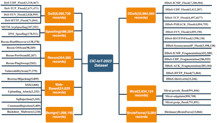
Figure 1: Count of attacks in the CICIoT2023 dataset. The count names of different types of attacks and benign records in the CICIot2023 dataset are described. These different types of attacks are broadly categorized into 7 attack classes. So there are a total of 8 classes, including benign in multiclass classification. Please click here to view a larger version of this figure.

Data preprocessing
Datasets should not be utilized in deep learning algorithms without sufficient preprocessing. Preprocessing is done to provide the algorithm with finer data, ultimately making the model more efficient. The output of the preprocessing pipeline-after label encoding, feature scaling, and feature selection-is termed "Final Data" and serves as the input to both CNN and Transformer components. The following steps are in Google Colab using Python. This research used Python 3.8.10, pandas 1.3.4, NumPy 1.21.4, scikit-learn 1.0.2, matplotlib 3.4.3, and TensorFlow/Keras 2.6.0 . The random seed was set to 42 for all runs.

Data acquisition
This step includes cleaning the data acquired from real-world contexts, since it often contains many errors and inconsistencies. If the dataset contains text values, for instance, it is impossible to utilise such values in deep learning training without first converting them to numerical form. When working with the dataset, the first thing that is done is to remove blank values and delete cells with no data in them. Rows with missing data were eliminated to avoid any adverse effects on the model.

The CIC-IoT-2023 dataset is loaded using pd.read_csv('ciciot2023_features_part.csv'). This research used Google Colab for model training and PySpark for initial cleaning. To detect missingness, the following methods are used: df.shape, df.info(), df.isnull().sum(), and df.duplicated().sum() for duplicates. Duplicates are eliminated using df.drop_duplicates(inplace=True). Numeric column type is verified using the formula df[col] = pd.to_numeric(df[col], errors='coerce'). If new NaNs appear, missing-value handling is reapplied. Features that are constant or nearly constant are also eliminated using df.drop(columns=low_variance_cols, inplace=True).

Label encoding
The next step is to transform the text labels into a numerical representation so the model can understand them. For binary classification, there are two separate kinds of labels. There are 46,686,579 records, with 45,588,384 labeled as malicious attacks. With 1,098,195 records included, the benign label is set to 0. There are seven separate types of attacks in multiclass classification. There are eight labels altogether, including the benign traffic. Figure 2 shows the count of each category of these labels. Multiclass mapping used in this research is: 0 for Benign, 1 for DoS, 2 for DDoS, 3 for recon, 4 for web-based attack, 5 for spoofing, 6 for bruteForce, and 7 for mirai attack.

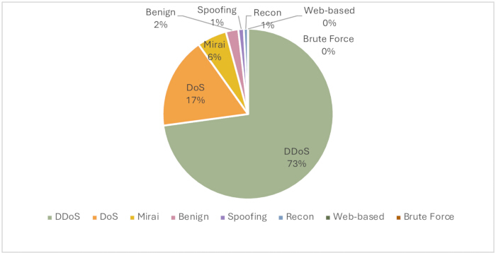
Figure 2: The percentage of attack classes including benign traffic. There are seven separate types of attacks in multiclass classification. There are eight labels altogether, including the benign traffic. The figure shows the count of each category of these labels. Please click here to view a larger version of this figure.

Feature scaling
Feature scaling is a common method for enhancing the overall performance of deep learning models. Feature scaling in this study is accomplished using Min Max Scaler and Standard Scaler technologies. The research did not use them for testing; instead, it only used the scaler on the training set to prevent data leakage. Data may be normalized to a zero-mean, one-standard-deviation distribution with the help of the Standard Scaler method. One way to do this is to divide the original number by the standard deviation. For this StandardScaler() function is called by importing StandardScaler from sklearn.preprocessing. By applying a range, often between 0 and 1, the Min Max Scaler normalizes the data. MinMaxScaler() function from scikit-learn was used to implement this.

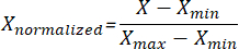
As indicated in Eq. (1), the normalizing formula is:

     (1)

Where X stands for the original point value and Xnormalized for its transformed form, Xmin represents the lowest value of the variable, while Xmax denotes the highest value of the variable within the data set.

Feature selection
Incorporating all characteristics from large datasets into training is not always helpful. Features inside the dataset may exhibit correlation and may not enhance the outcome. Furthermore, an excessive number of values escalates the expense of training. To find features that are not needed, we calculate their correlation matrices and exclude the ones with strong correlations from the dataset. Pearson's correlation coefficient, which quantifies the linear relationship between two features, is used to compute the correlation. A value between -1 and +1 is obtained by dividing the covariance of the two variables by the product of their standard deviations.This is optional and performed in the pipeline with Recursive Feature Elimination (RFE) for feature selection with a decision tree classifier. Recursive feature elimination repeatedly finds the most relevant features by training the classifier model and discarding the least significant ones. The code utilises RFE from sklearn.feature_selection with a Decision Tree Classifier as the estimator. Following the implementation of recursive feature elimination, 30 of the 46 characteristics have been picked for each of the seven attack categories, as shown in Table 2. A feature may be categorised under many attack classifications. Following the completion of the process outlined in Figure 3, the process of selecting the attack classes included within the dataset is carried out. Modern CNNs excel at learning hierarchical representations from raw data, but pre-selecting a small, high-quality feature set using RFE has significant advantages. First, RFE with a Decision Tree classifier quickly removes noisy or redundant data that might delay convergence during early training cycles. Second, centring the CNN on a smaller pool of actually valuable signals reduces overfitting, which is crucial in IoT traffic datasets with highly skewed benign and harmful patterns. The decision tree's recursive elimination method ranks features for better model explainability and identifying domain-specific biases before deep training. Finally, initializing the CNN-Transformer on this pruned feature set yields faster convergence and lower GPU memory use, proving that RFE actively accelerates and stabilizes end-to-end feature learning.

Table 2: The selected features of the dataset "CIC-IoT-2023". 30 of the 46 characteristics have been picked for each of the seven attack categories in this research using RFE. The table describes the selected 30 features. Please click here to download this Table.

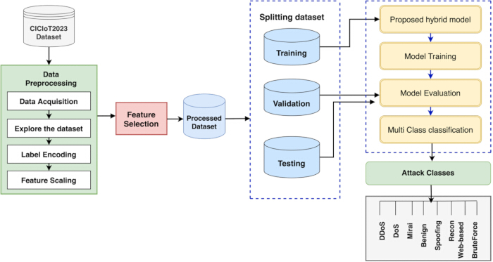
Figure 3: Working of the proposed hybrid model. The completion of the process is outlined in the figure. The process of selecting the attack classes included within the dataset is carried out. Please click here to view a larger version of this figure.

Split the dataset into an 80% train and a 20% test set by following the step: train_test_split (X_train, y_train, test_size=0.20, random_state=42). The 80% training set is further split using train_test_split(X_train, y_train, test_size=0.20,random_state=42). All model selection and hyperparameter tuning are done using these precise splits. The synthetic minority oversampling technique (SMOTE) is used when there is a class imbalance problem. Only the training set was subjected to SMOTE following splitting and scaling. The effect of SMOTE is presented in the results. Following RFE, the study parallels the CNN and Transformer branches using the same 30 features that were chosen for each sample. The further details of processing these 30 features are mentioned in the proposed methodology section.

Proposed methodology
An effective security framework for IoT systems that can more accurately detect attacks will be built with the help of a deep learning model. A hybrid security strategy that combines convolutional neural networks (CNNs) with transformer models is proposed. This method entails training the CNN architecture using weights from a bigger dataset and then fine-tuning the parameters of the model using a smaller dataset as a goal. The primary goal of this model is to improve the efficiency of intrusion detection in the IoT.

This research used PySpark, a Google Colab platform that allows users to run Python programs on Apache Spark. Using the Scikit-learn and Keras packages, deep learning algorithms have been developed. To train and test the model, the following configuration was used: Operating system: Mac OS v12.6; - M2 Apple Silicon; - 13.3-inch display; - 8-core CPU; - 8-core GPU; - 32 GB RAM; - 256 GB SSD.

The Canadian Institute for Cybersecurity (CIC) has created a comprehensive IoT threat dataset to advance security analysis applications in practical IoT environments³⁴. There were a total of 33 attacks on a network of 105 connected devices in an IoT system. With a total number of 46,179,314 incidents, attacks are categorized into seven groups: DDoS, Recon, DoS, web-based, spoofing, and brute force, in addition to Mirai. There are 37,349,263 instances in the training set, 8,830,051 instances in the test set, and a total of 46 characteristics in the dataset. In every instance, malevolent IoT devices launch attacks on other IoT devices. A total of 67 IoT devices and 38 Zigbee and Z-Wave devices connected to 5 hubs were affected by the attacks. A network of connected sensors, cameras, microcontrollers, and smart home devices may be set up to execute different types of attacks and record the traffic that results from them. Wireshark captures network traffic in PCAP format for further analysis. Since each experiment stores two streams of data, mergecap is used to combine the PCAP files. Various IoT devices were used to compile the dataset, including audio players, video recorders, hubs, power outlets, home automation systems, lighting, sensors, and NextGen gadgets.

This section gives a detailed research methodology consisting of many sequential phases used in the study. Furthermore, the part defines the proposed algorithm sequentially and provides a detailed flowchart of the research process.

CNN
The CNN algorithm uses an artificial neural network, a deep learning approach. Figure 4 illustrates the underlying algorithm that CNN uses: fully connected layers, pooling, flattening, and convolution are all a part of it. A CNN cannot function without the convolution layer. Receiving cell data is processed by the convolutional layer.

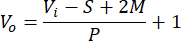
In Equation (2), the output volume (Vo) is determined by P (stride), Vi (input volume), S (convolutional layer neuron kernel size), and M (zero padding).

     (2)

After, a filter is used to extract the properties of the input value during convolution. This layer creates a feature map. Reducing input data size by pooling simplifies training and reduces the number of parameters to compute. The pooling layer may be chosen using either the largest value within the given size or the average of the values. The developed technique includes two layers of convolution and two levels of pooling. The feature extraction process begins here. The feature data that was obtained is made available for computation. CNN algorithms are available in one, two, or three dimensions. The model employed a convolutional neural network with just one dimension. The layers in the classifying area are known as flattened, fully connected. The data has to be flattened after the convolutional phase so it may be used in the fully connected phase. The flatten layer is where this process is carried out. Within the fully linked layer, the conventional paradigm of artificial neural networks is used. To apply CNN to the data that is not image-based, the input dimensions must be transformed. As a result, CNN may use one-dimensional convolutional layers that are one-dimensional³⁵.

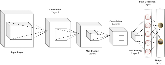
Figure 4: CNN basic algorithm. The basic working and components of the CNN model are described. Please click here to view a larger version of this figure.

Transformer learning
Furthermore, in order to carry out further experiments, we make use of the transformer modelling framework. The model can simultaneously handle all points in the sequence due to the transformer's self-attention mechanism. The result is a faster training time for the model and better use of computer resources by the transformer during inference and training. The transformer is primarily composed of a series of stacked encoders and decoders. The process of encoding involves changing one language into another, but the process of decoding involves determining the likelihood of a different language using previous outputs. Since encoders are mostly responsible for feature extraction, the suggested model exclusively uses encoder components. The transformer encoder consists of input/position embedding, a feedforward neural network, layer normalization, multi-head self-attention, and a residual network.

To prepare the input data for processing by the transformer, an embedding layer is used to convert the categorical characteristics into dense vector representations. Position embedding shows how features are connected sequentially, while input embedding shows how different inputs are related in a common space. Before the transformer processes categorical characteristics, this research uses input embedding to transform them into dense vectors.

An expansion of the attention mechanism, the multihead self-attention mechanism is the foundation of the transformer architecture. Using a scaled dot product, this research employs the multi-headed self-attention mechanism.

   (3)

where the query matrix (Q), key matrix (K), value matrix (V), and key matrix dimension (dk) are respectively denoted. By allowing the model to concentrate on data from various features mapped to separate subspaces, resulting in distinct attention values, a multi-head scaled dot-product attention mechanism varies from the scaled dot-product attention mechanism. Overfitting is less likely when attention levels are computed independently for each head. The specific formulation is as follows:

    (4)

(5)

Where h is the number of attention heads, d_v and d_model represent the dimension of v and model. Also,

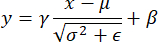
Next, layer normalization is used to stabilize the training process. To prevent gradient explosion, layer normalization limits the output of each layer to a certain range. Both the model's convergence and training speed may be improved by this. While batch normalization takes batch data into account, Layer normalization does not.

CNN-Transformer proposed model
This research offers a hybrid CNN-Transformer technique for detecting intrusions in IoT networks, considering the distinct benefits of both architectures. Figure 5 shows the main components of the proposed CNN-Transformer hybrid technique. After performing all preprocessing stages, including cleaning, normalization, label encoding, and feature selection, each sample in the dataset is represented by a 30-dimensional feature vector, which is called Final Data. The same Final Data is duplicated and fed in parallel to both branches of the hybrid model. Then, this Final Data is sent to both the CNN and Transformer blocks simultaneously. CNN and transformer do not rely on one another in any way; they may both work on the same input data at the same time. The flattened outputs of the two branches, CNN and Transformer, are concatenated to produce a fused feature vector, which is passed to the dense layers, which classify them. The CNN block changes the input shape to (num_features, 1) so that convolutional operations can be done across feature dimensions to find local spatial patterns. At the same time, the Transformer branch changes the same input into a sequential format and sends it to a higher-dimensional embedding space, followed by positional encoding. This lets the transformer pay self-attention in the feature space and find global contextual relationships. The transformer's unique design is used for feature extraction, while the sigmoid function and completely linked layers provide the mapping connection between features and labels. The CNN-Transformer model is structurally represented by Figure 5. The result is an eight-category system for classifying attacks, with DDoS, Recon, DoS, Benign, Web-based, Spoofing, Brute Force, and Mirai as component parts. The evaluation process of the proposed CNN-Transformer is shown in Figure 5.

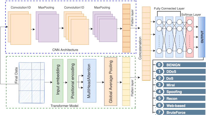
Figure 5: Architecture of proposed model. The figure shows the input shape and evaluation process of the proposed CNN-Transformer. Please click here to view a larger version of this figure.

Two one-dimensional convolutional neural networks (CNNs) with 64- and 128-unit filters and a 3-kernel size, two max-pooling layers, a flattening step, three dense layers with 256, 128, and 64 units, and three dropout layers make up the convolutional neural network (CNN) layer.

The input data is processed via a 1D convolutional layer with a ReLU activation function, 64 filters, a 3x3 kernel, and a 1x1 stride in the first layer. Following the preceding layer is a MaxPooling1D layer with a pool size of 2. In order to make the model more flexible and to decrease its computational cost, this layer decreases the spatial dimensions of the output area. Layer three is yet another 1D convolutional layer; it has 128 filters, a kernel of three sizes, a stride of one, and an activation function named ReLU. Using more filters to extract input characteristics, this layer is similar to the first max pooling layer. The first layer's output is then processed using the technique. Afterwards, a maximum pooling layer was added after the second convolution layer, and its pool size was also 2. Once again, this layer is used to downsample the feature maps. The fifth layer is a flattening layer, and it takes the output from the previous layer and makes it into a one-dimensional vector.

The obtained feature subsets are input embedded as a last step before becoming the transformer's input. In addition, multi-head attention -- a one-dimensional vector of eight heads with a 32-key dimension -- is used to assess the significance of each head. The multi-head attention layer is the main component of the transformer. This layer allows the model to learn from the embedded representations of different characteristics in an adaptive way. The multi-head attention layer is made up of several self-attention heads, which are also called "scaled dot-product attention". Subsequent to applying layer normalization with epsilon set to 1e-6, the objective is to eradicate scale discrepancies among various characteristics and ensure output stability. By keeping each layer's output within a predetermined range, layer normalization lessens the likelihood of gradient explosion. Following the transformer's output is a flattening layer, which simplifies its combination with the CNN by reducing it to a single vector.

The next step is to combine the CNN and Transformer's flattened outputs using a concatenation layer. Activation function "relu," L2 regularisation, and a dense layer with 256 units follow the flatten layer. This is followed by a dropout layer with a rate of 0.5, which helps avoid overfitting. An additional 128-unit dense layer using L2 regularization and the "relu" activation function follows. The dropout rate in an additional dropout layer is 0.3. ReLU activation function, L2 regularization, and a 64-unit dense layer comprise the subsequent layer. The next layer takes the form of a 0.2 rate dropout layer, randomly eliminating 20% of the units inside. A dense layer with a softmax activation function creates a probability distribution for the last layer's output classes. There are exactly as many units in this layer as there are output classes.

The suggested model may be expressed numerically as follows:
Let X be the CNN input data, where X R^(n×1), after reshaping, and n is the number of selected features, respectively. X is put into a higher-dimensional embedding space of shape R^{(n × d_model)} for the Transformer block. Before it goes into the self-attention mechanism, positional encoding is used.

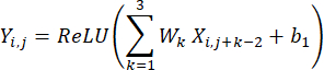
The following is the expression of the operation in the Conv1D layer, which uses 64 filters and a kernel size of 3:

   (6)

where Y_i,j is the output at position j of the i_th filter, k is the kernel of size 3, b₁ R⁶⁴ is the bias term for each filter, W_k represents filter weights, and ReLU is the activation function. Next, the MaxPooling layer is applied with a pool size of 2, giving an output Z_1,j.

   (7)

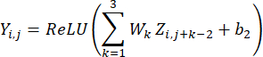
An extra ID convolution layer with a 3 kernel size and 128 filters is included as the model's third layer; its expression is:

   (8)

Where k is the kernel of size 3, b₂ R¹²⁸ is the bias term for each filter, and ReLU is the activation function. Another max pool layer is applied, getting the input from the second convolution layer with a pool size of 2. The output Z_2,j is given by:

   (9)

The fifth layer is a flattening layer expressed as:

   (10)

Next are the transformer layers, which include an embedding layer, a multi-head attention layer, and layer normalization

    (11)

E is the embedding vector for input class label c, and W_e is the weight matrix containing embedding vectors for all categories. This maps each integer in c to a dense vector of 32 real-valued components. Next is a multi-head attention layer, as formulated in Equation (3),(4) and (5).

The key matrix has a size of d_k =32 and a dimension of h=8. d_v and d_model stand for v's and model's respective dimensions. Also,

For an output x = MultiHead(Q,K,V), layer normalization provides:

    (12)

Where y is the normalized output, γ and β are the learnable parameters, and µ and σ² denote the mean and variance for x, respectively. Next is the flattening layer for the transformer, defined as

At the end of all the layers, the resultant expression is shown as

Where Z₁R²⁵⁶, Z₂R¹²⁸, Z₃R⁶⁴, and YR⁸. This hybrid model also calculates the loss function for multiclass classification, which can be expressed as

where:
Y_c represents the true label (one-hot encoded) for class cc,
Y'_c is the predicted probability for class c
The proposed algorithm is explained in Table 3 in detail.

Table 3: The proposed CNN-Transformer algorithm. The proposed algorithm is explained in Table 3 step by step. Please click here to download this Table.

Results

This section presents the evaluation parameters along with the test results.

Performance evaluation metrics
The effectiveness of the models may be evaluated using several defined criteria for evaluation. Accuracy, recall, precision, F1 score, ROC, confusion matrix, and other statistical metrics are shown in Table 4. Insights into the models' overall performance are provided by the metrics.

Table 4: Performance evaluation...

Discussion

The CNN-Transformer model was tested on the CICIoT2023 datasets, with 80% reserved for training and 20% for testing. The model achieved an accuracy of 99.97%, F1 score of 99.96%, recall of 99.97%, precision of 99.96% and a loss of 0.0123, confirming its effectiveness for IoT intrusion detection. CNN-based approaches, similar to the findings¹³, are proficient in detecting small spatial patterns within network traffic characteristics; however, they often exhibit constraints in modeling long-range de...

Materials

List of materials used in this article

Name	Company	Catalog Number	Comments
Apple M2 (8-core CPU)	Apple	N/A	(OS) provides the environment in which deep learning frameworks and tools operate.
CICIoT2023 Dataset	UNB	https://www.unb.ca/cic/datasets/iot2023.html	Publically available daset of IoT
Keras 2.6.0	Keras	https://keras.io/	An API running on top of TensorFlow, providing a user-friendly interface.
Matplotlib 3.4.3	Matplotlib	https://matplotlib.org/	Visualization library for Python.
NumPy 1.21.4	Numpy	https://numpy.org/	Fundamental package for scientific computing with Python
NVIDIA Tesla P100 GPU (16 GB VRAM)	Google Colab Pro	N/A	Training hardware
Pandas 1.3.4	Pandas	https://pandas.pydata.org/	Data analysis and manipulation tool.
Python 3.8.10	Python Software Foundation	https://www.python.org/downloads/release/python-3810/	The most popular language for deep learning due to its extensive libraries and community support.
scikit-learn 1.0.2	Scikit Learn	https://scikit-learn.org/	Machine learning library for Python.
Seaborn 0.11.2	Seaborn	https://seaborn.pydata.org/	Statistical data visualization library.
System RAM	N/A	N/A	32 GB RAM
TensorFlow 2.6.0	Google	https://www.tensorflow.org/	Widely used for its comprehensive tools and libraries.

References

- Abbas, S., et al. A novel federated edge learning approach for detecting cyberattacks in IoT infrastructures. IEEE Access. 11, 112189-112198 (2023).
- Asharf, J., et al. A review of intrusion detection systems using machine and deep learning in internet of things: challenges, solutions and future directions. Electronics. 9 (7), 1177(2020).
- Qiu, J., Tian, Z., Du, C., Zuo, Q., Su, S., Fang, B. A survey on access control in the age of internet of things. IEEE Internet Things J. 7 (6), 4682-4696 (2020).
- Zhang, K., et al. Compacting deep neural networks for internet of things: methods and applications. IEEE Internet Things J. 8 (15), 11935-11959 (2021).
- Farooq, U., Tariq, N., Asim, M., Baker, T., Al-Shamma'a, A. Machine learning and the internet of things security: solutions and open challenges. J Parallel Distrib Comput. 162, 89-104 (2022).
- Regan, C., et al. Federated IoT attack detection using decentralized edge data. Mach Learn Appl. 8, 100263(2022).
- Sarhan, M., Layeghy, S., Moustafa, N., Portmann, M. Cyber threat intelligence sharing scheme based on federated learning for network intrusion detection. J Netw Syst Manage. 31 (1), (2023).
- Verma, P., et al. A novel intrusion detection approach using machine learning ensemble for IoT environments. Appl Sci. 11 (21), 10268(2021).
- Rajagopal, S., Kundapur, P. P., Hareesha, K. S. A stacking ensemble for network intrusion detection using heterogeneous datasets. Secur Commun Netw. 2020, 4586875(2020).
- Enhancing IoT security with CNN and LSTM-based intrusion detection systems. Gueriani, A., Kheddar, H., Mazari, A. C. Proc Int Conf Pattern Anal Intell Syst, 6, 1-7 (2024).
- Nandanwar, H., Katarya, R. Deep learning enabled intrusion detection system for industrial IoT environment. Expert Syst Appl. 249, 123808(2024).
- Jony, A. I., Arnob, A. K. B. A long short-term memory based approach for detecting cyber attacks in IoT using CIC-IoT2023 dataset. J Edge Comput. 3 (1), 28-42 (2024).
- de Caldas Filho, F. L., et al. Botnet detection and mitigation model for IoT networks using federated learning. Sensors. 23 (14), 6305(2023).
- Wang, Z., et al. ThreatInsight: innovating early threat detection through threat-intelligence-driven analysis and attribution. IEEE Trans Knowl Data Eng. 36 (12), 9388-9402 (2024).
- Chai, Y., Du, L., Qiu, J., Yin, L., Tian, Z. Dynamic prototype network based on sample adaptation for few-shot malware detection. IEEE Trans Knowl Data Eng. 35 (5), 4754-4766 (2023).
- Shah, H., et al. Deep learning-based malicious smart contract and intrusion detection system for IoT environment. Mathematics. 11 (2), 418(2023).
- Luo, C., et al. A novel web attack detection system for internet of things via ensemble classification. IEEE Trans Ind Inform. 17 (8), 5810-5818 (2021).
- Tian, Z., et al. A distributed deep learning system for web attack detection on edge devices. IEEE Trans Ind Inform. 16 (3), 1963-1971 (2020).
- Chai, Y., et al. MalFSCIL: a few-shot class-incremental learning approach for malware detection. IEEE Trans Inf Forensics Secur. 20, 2999-3014 (2025).
- Maghrabi, L. A. Automated network intrusion detection for internet of things: security enhancements. IEEE Access. 12, 30839-30851 (2024).
- He, M., et al. Reinforcement learning meets network intrusion detection: a transferable and adaptable framework for anomaly behavior identification. IEEE Trans Netw Serv Manage. 21 (2), 2477-2492 (2024).
- Oseni, A., et al. An explainable deep learning framework for resilient intrusion detection in IoT-enabled transportation networks. IEEE Trans Intell Transp Syst. 24 (1), 1000-1014 (2023).
- Khan, F., et al. Trustworthy and reliable deep-learning-based cyberattack detection in industrial IoT. IEEE Trans Ind Inform. 19 (1), 1030-1038 (2023).
- IoT anomaly detection using a multitude of machine learning algorithms. Balega, M., et al. Proc IEEE Appl Imagery Pattern Recognit Workshop, 2022, 1-7 (2022).
- A hybrid machine learning approach to anomaly detection in industrial IoT. Jayesh, T. P., et al. Proc Int Conf Adv Comput Commun Embedded Syst, 3, 32-36 (2023).
- Mezina, A., Burget, R., Travieso-Gonzalez, C. M. Network anomaly detection with temporal convolutional network and U-Net model. IEEE Access. 9, 143608-143622 (2021).
- Ahmad, Z., et al. Anomaly detection using deep neural network for IoT architecture. Appl Sci. 11 (15), 7050(2021).
- Raman, M., et al. An efficient intrusion detection technique based on support vector machine and improved binary gravitational search algorithm. Artif Intell Rev. 53, (2020).
- Thaseen, I. S., et al. A hadoop based framework integrating machine learning classifiers for anomaly detection in the internet of things. Electronics. 10 (16), 1955(2021).
- Almiani, M., et al. Deep recurrent neural network for IoT intrusion detection system. Simul Model Pract Theory. 101, 102031(2020).
- A novel approach to detect IoT malware by system calls using deep learning techniques. Shobana, M., Poonkuzhali, S. Proc Int Conf Innovative Trends Inf Technol, 2020, 1-5 (2020).
- Farsi, M. Application of ensemble RNN deep neural network to the fall detection through IoT environment. Alex Eng J. 60 (1), 199-211 (2021).
- Tseng, S. M., Wang, Y. Q., Wang, Y. C. Multiclass intrusion detection based on transformer for IoT networks using CIC-IoT-2023 dataset. Future Internet. 16 (8), 284(2024).
- Neto, E. C. P., et al. CICIoT2023: a real-time dataset and benchmark for large-scale attacks in IoT environment. Sensors. 23 (13), 5941(2023).
- Tsimenidis, S., Lagkas, T., Rantos, K. Deep learning in IoT intrusion detection. J Netw Syst Manage. 30 (1), 8(2021).
- Kamal, H. Advanced hybrid transformer-CNN deep learning model for effective intrusion detection systems with class imbalance mitigation using resampling techniques. Future Internet. 16 (12), 481(2024).
- Alghieth, M. DeepECG-Net: a hybrid transformer-based deep learning model for real-time ECG anomaly detection. Sci Rep. 15 (1), 20714(2025).
- Kethineni, K., Pradeepini, G. Intrusion detection in internet of things-based smart farming using hybrid deep learning framework. Clust Comput. 27 (2), 1719-1732 (2024).
- Alharbi, A., et al. Botnet attack detection using local global best bat algorithm for industrial internet of things. Electronics. 10 (11), 1341(2021).
- Kunang, Y. N., et al. Attack classification of an intrusion detection system using deep learning and hyperparameter optimization. J Inf Secur Appl. 58, 102804(2021).
- Han, W., et al. Heterogeneous data-aware federated learning for intrusion detection systems via meta-sampling in artificial intelligence of things. IEEE Internet Things J. 11 (8), 13340-13354 (2024).
Access restricted. Please log in or start a trial to view this content.