Bioinformatics Approach to Cancer Prediction using Quantum Clustering Algorithm for Behavioral Similarity in Gene Expression

Summary

This protocol aims to cluster gene expression data for cancer classification using a Hybrid Quantum K-Means algorithm that automatically detects the optimal number of clusters and separates them efficiently, advancing bioinformatics applications on Noisy Intermediate-Scale Quantum ( NISQ) devices.

Abstract

This study introduces a Hybrid Quantum K-Means Clustering Algorithm with automatic cluster detection for classifying cancerous and non-cancerous gene expression data. The method employs Quantum Multi-Feature Mapping for state encoding, Swap Test-based quantum distance estimation, and Quantum Gradient-Based Optimization to dynamically identify the optimal number of clusters by minimizing intra-cluster variance. Initial centroids are selected through a probability-proportional distance strategy, improving stability and accuracy. Applied to breast cancer datasets, the approach surpasses the existing quantum K-Means algorithm, achieving a Silhouette Score of 0.641 (compared to 0.601), a Calinski-Harabasz Index of 766.57 (compared to 617.65), and a Davies-Bouldin Index of 0.659 (compared to 0.704). These results indicate superior cluster compactness and separation. Although the proposed algorithm exhibits slightly higher time complexity O (N×K_max×M_obs) due to iterative optimization, it significantly outperforms predefined-K quantum K-Means in clustering accuracy, error reduction, and practical feasibility. Its efficiency in handling high-dimensional data and resilience to quantum noise highlights its potential for real-world bioinformatics applications, particularly in cancer classification using gene expression profiles.

Introduction

In biomedical engineering, bioinformatics, statistics, social sciences, and economics, clustering is a fundamental technique for organizing data into meaningful homogeneous groups. For example, topological data analysis (TDA) has been applied to cancer gene expression datasets to reveal structural patterns in high-dimensional spaces¹, Clustering organizes data such that objects with high similarity are placed within the same cluster, while dissimilar objects are assigned to different clusters. This falls under unsupervised learning and does not require labeled training data.

Over the past several decades, numerous clustering algorithms have been developed. Classical approaches include partition-based clustering²˒³, density-based clustering^4,5, hierarchical clustering^6,7, grid-based clustering⁸˒⁹, and model-based clustering¹⁰. Reviews of these methods highlight their strengths but also their limitations¹¹. While effective in specific contexts, most classical algorithms struggle with high-dimensional, noisy, or irregularly distributed data. Consequently, no universal clustering method exists that performs optimally across all data types.

To address these challenges, quantum clustering has emerged as a promising alternative¹². Unlike classical algorithms, quantum-inspired approaches leverage superposition, entanglement, and other principles of quantum mechanics to explore data spaces more efficiently. This paradigm has become increasingly accepted within the research community¹³˒¹⁴˒¹⁵˒¹⁶˒¹⁷˒¹⁸, as it demonstrates potential advantages over classical clustering in handling high-dimensional and noisy datasets. Nevertheless, existing quantum clustering methods often suffer from predefined cluster counts or unstable centroid initialization, which reduce their robustness in practical applications.

In this work, a novel partition-based Hybrid Quantum K-Means Clustering algorithm is introduced, incorporating four distinct innovations: (i) Quantum Multi-Feature Mapping for encoding gene expression data into high-dimensional Hilbert space; (ii) probability-proportional distance-based centroid initialization, improving stability compared to random initialization; (iii) Swap Test-based quantum distance estimation for accurate similarity measurement; and (iv) Quantum Gradient-Based Optimization to dynamically determine the optimal number of clusters by minimizing intra-cluster variance. These contributions distinguish the proposed method from prior quantum clustering approaches^19,20, enhancing robustness, scalability, and applicability in real-world bioinformatics scenarios.

Clustering gene expression data is a critical task in bioinformatics, particularly for distinguishing between cancerous and non-cancerous cells based on their genetic profiles. Traditional clustering methods, such as classical K-Means, often struggle with the high-dimensional nature of gene expression datasets, leading to suboptimal classification. To overcome these challenges, we introduce the Quantum K-Means Algorithm with Optimal Cluster Determination, which leverages Quantum Feature Mapping and probabilistic centroid initialization to achieve superior clustering performance. This algorithm not only clusters the gene expression data efficiently but also automatically determines the optimal number of clusters, enabling the identification of distinct cancer subtypes

The proposed algorithm is applied to datasets containing both cancerous and non-cancerous gene expression profiles, clustering them based on behavioral similarity to evaluate its effectiveness.

Protocol

1. Quantum Feature Mapping

Encoding classical data points into quantum states is achieved by mapping them into a quantum Hilbert space, which can be efficiently accessed and manipulated by a quantum computer¹⁶˒^17,19. This process employs a nonlinear quantum feature map that embeds classical data into the Hilbert space (Figure 1). A fixed quantum circuit feature map transforms the input data points into quantum states¹⁷, while variational circuits enable machine learning tasks by adapting the measurement basis²². A variational circuit consists of a set of parameterized quantum gates, optimized through hybrid quantum-classical techniques²³.

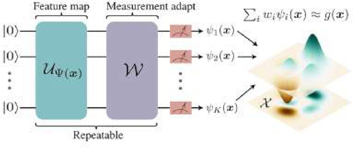
Figure 1: Feature mapping in Quantum Hilbert Space. Please click here to view a larger version of this figure.

2. Encoding Target Point and Centroids into qubits

For encoding the features of our data points, we need to perform rotations using U3 gates.

This rotates the qubit θ radians away from the positive z-axis, and Φ radians from the positive x-axis.

All qubits were initialized in the ∣0〉 state before the encoding process began. Each gene expression value was normalized to the range [0,1] and converted into a rotation angle using the relation θ_i=πx_i. A parameterized unitary gate was then applied to each qubit to encode the corresponding feature, implemented in Qiskit using the operation qc.u(theta_i, pi, pi, qubit_index). When multiple features were encoded, the rotation procedure was repeated across the appropriate qubits to create a multi-feature representation. After these operations, the resulting quantum state ∣ψ〉 represented the encoded feature vector in Hilbert space. No measurement was performed during this stage, as the prepared state was reserved for subsequent similarity estimation.

3. Comparing Quantum States

The outcomes of quantum experiments are inherently random because qubits are unstable by nature, as described in quantum physics. Consequently, conclusions and predictions must be expressed in terms of probabilities and uncertainties. Drawing unambiguous conclusions therefore presents a genuine challenge. However, when the quantum states under consideration are pure, differences between states (with nonzero probability) can be predicted unambiguously through experimentation²⁴˒²⁵.

Two quantum states, ∣ψ〉 and ∣ϕ〉, were first loaded into separate quantum registers. An ancilla qubit was then initialized in the ∣0〉 state to control the swap operation. A Hadamard gate was applied to the ancilla to place it in superposition before the controlled-SWAP operation was executed. The Fredkin (CSWAP) gate used the ancilla as the control qubit and the two data registers as targets, enabling interference between the states. After this operation, a second Hadamard gate was applied to the ancilla to complete the interference pattern. Only the ancilla qubit was measured, and its measurement outcome encoded the similarity between the two states. When the states were identical, the ancilla yielded the outcome 0 with probability 1, whereas orthogonal states produced the outcome 0 with probability 0.5.

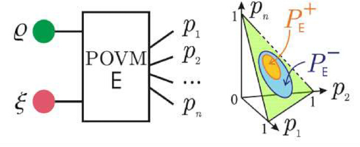
Figure 2: Illustration of probability-based comparison, If states ρ and ξ are different then the observed probability distribution belongs to P_E⁻ \ P_E⁺. Please click here to view a larger version of this figure.

The density operator ρ is associated with any quantum state ρ ∈ S(H), such that tr[ρ] = 1 and ρ ≥ 0. Here, set of all state S(H) of a system which will associated with the Hilbert space H. Positive Operator Valued Measure (POVM) is a quantum statistical features measurement which is a collection of positive operators E₁, . . . , E_n as E (which acting on H) and the identity I = . A probability distribution assigns the measurement E for each state ρ ∈ S(H) where p_j = tr[E_jρ]≥ 0 and = 1²⁶.

4. SWAP-based Comparing Quantum States

The difference between two quantum states can be measured using the SWAP test procedure in quantum computation. This method was first introduced by Barenco et al.²⁷ and later rediscovered by John Watrous, Ronald de Wolf, Harry Buhrman, and Richard Cleve ²⁸. The SWAP test has been applied to quantum computing and quantum machine learning ^15,29.

The SWAP test takes ∣ψ〉 and ∣ϕ〉 as input states and outputs 1 (a Bernoulli random variable) with probability ½ - ½〈ϕ,ψ〉² which estimates the squared inner product of the two states ³⁰.

Explanation of Circuit

Consider two states ∣ϕ〉 and ∣ψ〉 of the system, the protocol at the beginning is ∣0,ϕ,ψ〉. After applying the Hadamard gate, the state is changed to ∣0,ϕ,ψ〉 + ∣1,ϕ,ψ〉. The CSWAP gate transforms the state into (0,ϕ,ψ〉 + ∣1,ψ,ϕ〉). After the second Hadamard gate, the state becomes ½(|0,ϕ,ψ〉 + ∣1,ϕ,ψ〉 + |0,ψ,ϕ〉 - ∣1,ψ,ϕ〉)= ½∣0〉(|ϕ,ψ〉 + |ψ,ϕ〉) +  ½|1〉(|ϕ,ψ〉 - |ψ,ϕ〉). The first qubit is then measured, the probability of obtaining outcome 0 is P(First qubit = 0) = ½ (〈ϕ|〈ψ| + 〈ψ|〈ϕ|) ½ (|ϕ,ψ〉 + |ψ,ϕ〉) = ½ + ½ |〈ψ|ϕ〉|². If ψ and ϕ are orthogonal (|〈ψ|ϕ〉|² = 0), then the probability of obtaining 0 is ½. If the states are identical (|〈ψ|ϕ〉|² = 1) then the probability of obtaining 0 is 1.²⁴

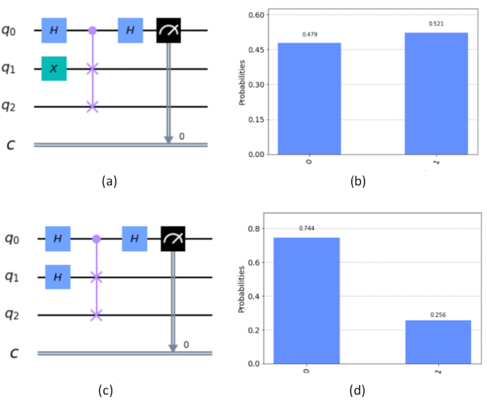
Figure 3: (a) Circuit of Fredkin gate with polar opposite state, (b) Output of probability measured graph, (c) Circuit of Fredkin gate with Hadamard gate, (d) Output of probability measured graph. Please click here to view a larger version of this figure.

The circuit used one ancilla qubit along with two registers that encoded the quantum states ∣ψ〉 and ∣ϕ〉. All qubits were initialized before the encoding stage began. The gene expression features were then encoded into the respective registers using the feature-mapping procedure. A Hadamard gate was applied to the ancilla qubit to create a superposition, after which a controlled-SWAP operation was performed between the two state registers with the ancilla as the control. A second Hadamard gate was applied to the ancilla to complete the interference pattern, and the ancilla qubit was subsequently measured. When the two encoded states were identical, the ancilla consistently produced the outcome 0. When the states were orthogonal, the ancilla yielded the outcome with probability 0.5. For partially similar states, the probability of obtaining 0 lay between 0.5 and 1, reflecting the degree of similarity between the states.

5. Quantum Distance Estimation

In classical data analysis, distances between data points can be computed directly using measures such as Euclidean or Manhattan distance ^2,3. In the case of qubits on a quantum computer, this task is more complex due to the probabilistic nature of quantum states. While phase differences and probability amplitudes can be measured, they cannot be directly represented as distances between two vectors ^24,26.

For clustering, it is necessary to evaluate the relative positions of data points with respect to cluster centroids¹³. To assign each qubit to the appropriate cluster, a parameter must be defined that serves as an indicator of proximity to the corresponding cluster centroid.

To achieve this, a parameter is introduced that correlates positively with similarity, thereby functioning as an alternative to conventional distance measures ^15,30.

The distance estimation process began with a normalized quantum state ∣Ψ〉 and a zero-initialized ancillary qubit ∣q₀〉. The objective was to estimate the distance between the new data point encoded in ∣q₁〉 and a cluster centroid encoded in ∣q₂〉. To prepare the superposition required for the interference pattern, a Hadamard gate was applied to the ancilla qubit, producing the state ( ∣0〉 + ∣1〉 ) ⊗ ∣Ψ〉 ). A controlled-SWAP (Fredkin) gate was then applied with the ancilla as the control, which entangled the ancilla with the two encoded states and enabled their overlap to influence the measurement outcome. This operation produced the state ( ∣0〉 ⊗ ∣Ψ〉 + ∣1〉 ⊗ F_swap(∣Ψ〉) ), from which the inner-product-based distance could be extracted through subsequent measurement of the ancilla.

Circuit Implementation & Output

This quantum circuit encodes gene expression data into qubits using phase encoding and subsequently compares two gene expression states through the Controlled-Swap (CSwap) gate, also known as the Swap Test¹².

To create the required superposition, Hadamard gates are applied to all qubits (q₀ to q₄), resulting in an equal superposition of all basis states |Ψ〉 = 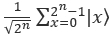, This initialization enables parallel computation over multiple gene expression values. Each qubit then undergoes a phase rotation, , where θ_x corresponds to the mapped gene expression value. The unitary operators U(θ,π,π) applied to qubits q₁-q₄ encode the expression levels of individual genes, with each angle θ representing a transformed version of a gene's expression. This procedure maps classical biological data into quantum states through phase encoding, allowing multiple genes to be represented in a high-dimensional quantum space⁶.

The CSwap gates are then used to compare encoded states by entangling them. The ancillary qubit q₀ acts as the control, determining whether the states of q₁-q₄ are swapped. Similar quantum states generate constructive interference in q₀, resulting in a higher probability of measuring ∣0〉. Conversely, dissimilar states increase the probability of measuring ∣1〉. A subsequent Hadamard gate on q₀ ensures amplitude interference, enabling the extraction of similarity information through measurement.

Suppose two quantum states ∣ψ〉 and ∣ϕ〉 represent distinct gene expression datasets, |ψ〉 = ∑_ia_i |i〉, |ϕ〉 = ∑_ib_i |i〉 .

The Swap Test evaluates the fidelity (inner product) between them:

P (0) = ,

Where ∣〈ψ∣ϕ〉∣ denotes the inner product. If P(0) ≈ 1, the states are similar; if P(0) ≈ 0.5 or lower, they are dissimilar.

This framework enables comparison of datasets across patients or experimental conditions (e.g., normal vs. diseased tissue). It provides an efficient basis for clustering high-dimensional data within quantum machine learning models. The Swap Test supports identification of similarities between quantum states, which can be utilized for grouping samples into meaningful clusters⁴.

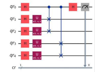
Figure 4: Circuit of measuring distance between data points and centroids. Please click here to view a larger version of this figure.

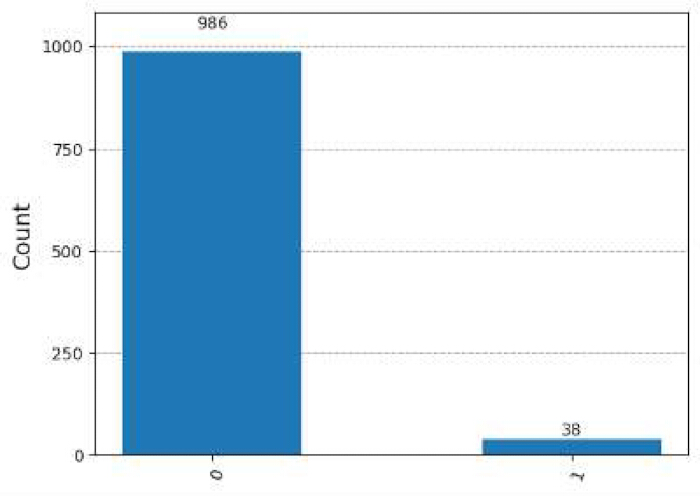
Figure 5: Output of probability measured graph. Please click here to view a larger version of this figure.

A data point was first encoded into the quantum state ∣ψ〉 and the corresponding cluster centroid was encoded into the state ∣ϕ〉. The swap test procedure described earlier was then executed to compare these two states, and the ancilla measurement probability P(0) was recorded. The fidelity between the states was obtained as F=∣〈ψ∣ϕ〉∣², and the quantum distance was defined as D (ψ,ϕ) = . A smaller value of D indicated that the data point was closer to the centroid in the quantum feature space.

6. Initial Centroid Selection

The initialization of cluster centroids is critical for the stability and accuracy of K-Means clustering. Randomized selection may produce poorly distributed centroids, leading to slow convergence and suboptimal results. To address this issue, a probability-proportional distance method inspired by the K-Means++ strategy²⁰ is employed. In the quantum-enhanced approach, distances are evaluated using the Quantum Distance Estimator based on the SWAP test, ensuring that the selected centroids better represent the underlying data distribution. This strategy enhances cluster separation and improves algorithmic robustness, particularly in high-dimensional datasets.

The centroid initialization process began by selecting one data point at random to serve as the first centroid. The quantum distance between this centroid and every remaining data point was then computed using the quantum distance estimation procedure. Based on these distance values, a probability distribution was created in which each point was assigned a selection probability proportional to its squared distance from the nearest centroid. New centroids were sampled according to this distribution, and the procedure was repeated until the desired number of centroids K was obtained. This approach produced an initial centroid set with substantially better separation than random selection.

7. Quantum Variance Calculation

Cluster variance quantifies the compactness of data points around their centroids, making it a crucial metric for evaluating clustering quality. In classical K-Means, variance is computed as the mean squared distance between data points and their assigned centroids. In the quantum-enhanced approach, these distances are obtained using the Quantum Distance Estimator (via the SWAP test), which computes fidelity-based similarities between quantum states. By summing squared distances within each cluster and normalizing by cluster size, we obtain a variance value that reflects the degree of intra-cluster cohesion. Minimizing this variance ensures tighter, more meaningful clusters, which is particularly important in high-dimensional gene expression datasets for distinguishing cancerous and non-cancerous samples.

Cluster assignment was performed by assigning each encoded quantum data point to the nearest centroid using quantum distance estimation. For every cluster C_k, the quantum distance D(ψ_i,C_k) between each data point and its centroid was computed. The within-cluster variance was then calculated using  , which measured the compactness of each cluster. The total variance was obtained by summing the individual variances across all clusters. This total variance value was recorded for determining the optimal number of clusters and for evaluating the overall clustering performance.

8. Quantum Gradient-Based Optimization

Determining the optimal number of clusters (K) is a fundamental challenge in clustering tasks. Traditional K-Means requires K to be predefined, often leading to under- or over-clustering. In our quantum-enhanced approach, we integrate Quantum Gradient-Based Optimization (QGBO) to adaptively identify the optimal cluster count. The algorithm iteratively increases K, recalculates the variance at each step, and evaluates the reduction in variance (ΔV). When improvements in variance fall below a threshold, clustering is terminated. The quantum gradient is computed using the parameter-shift rule, which estimates derivatives of expectation values from quantum circuits. This approach ensures that the final number of clusters balances accuracy and efficiency, making it particularly useful in bioinformatics applications where the true number of biological subtypes is not known in advance.

The clustering process began with K=1, and the total variance V(K) was computed using the quantum variance calculation procedure. The number of clusters was then increased to K+1, and the variance V(K+1) was recalculated. The reduction in variance, ΔV=V(K)−V(K+1), was evaluated to determine whether additional clusters continued to improve the compactness of the data. The iteration stopped when ΔV fell below the predefined threshold, indicating that further increases in K did not yield meaningful improvements. A parameterized quantum circuit with variational gates was constructed to monitor curvature changes in the variance trend, and this information guided the cluster optimization process. The optimal number of clusters was selected as the value of K at which the variance reduction stabilized, resulting in compact and well-separated clusters.

9. Calculating Cluster Variance and Storing in V_list

Once stable clusters are formed, the algorithm calculates the cluster variance to measure the compactness of each cluster. The variance V_kj for a given cluster is determined using the distances between each data point in the cluster and the cluster centroid:

where: x represents a gene expression sample, C_i represents a cluster, C_ci is the centroid of cluster C_i, V_kj represents the variance recorded for the j^th iteration with k clusters.

This variance is stored in a list V_list, which will later be used to determine the optimal number of clusters.

10. Determining the Optimal Number of Clusters

To find the optimal number of clusters K, the algorithm performs multiple iterations, observing different starting conditions. The key steps include:

The algorithm first identified the minimum variance value from the list of variances computed for different values of K. The reduction in variance between successive cluster counts was then measured using the expression ΔV=∣V_k−V_k−1∣, where V_k denoted the variance for K clusters and V_k−1 represented the variance for K−1 clusters. If the reduction ΔV fell below the predefined threshold, indicating a negligible improvement in clustering, the procedure terminated. Otherwise, the number of clusters was incremented, and the computation was repeated until the optimal cluster count was reached.

11. Finalizing Clusters for Cancer and Non-Cancer Classification

Once the optimal number of clusters K is determined, the final set of clusters represents distinct groups within the gene expression data. Typically, the algorithm results in two primary clusters:

One cluster representing cancerous cells (marked by distinct gene expression signatures associated with malignancy).

One cluster representing non-cancerous cells (containing normal gene expression profiles).

The parameters, variables, and constants employed in the proposed Quantum K-Means clustering algorithm are listed in Table 1. Define the dataset dimensions, set the number of clusters K, and apply stopping criteria and optimization thresholds to guide the process. Configure computational settings such as the number of shots per run and random seed to ensure reproducibility. Initialize centroids using a probability-based selection method and update them iteratively until convergence. The table also specifies the expected outputs, including cluster labels, centroids, optimal K, evaluation metrics, and visualization plots.

Category	Parameter	Value / Default	Notes
Dataset	Breast cancer dataset	569 samples × 32 features (reduced to 2 PCA components)	Dimensionality reduced with PCA
Number of clusters	K	Dynamic, initially 1, up to 5	Optimized using variance reduction
Maximum clusters	Kmax	5	Upper bound for search
Shots per run	N	1024	Measurements per circuit execution
Stopping tolerance	ε	1 × 10^-14	Variance convergence criterion
Variance slope threshold	ΔV	9.9 × 10^-4	Stopping threshold for optimization
Observations	Mobsrv	3	Independent runs per cluster size
Iteration limit	–	10	Maximum centroid update steps per run
Random seed	–	42	Ensures reproducibility
Expected outputs	–	Cluster labels, centroids, optimal K, evaluation metrics, plots	Exported as .csv and .png files
Variances across clusters	Vlist	empty	Detects optimal K
Centroid j	cj	initialised by function (based on probabilities proportional to the squared distances of points)	Updated iteratively and and store final centroids

Table 1: Materials, Software, and Reproducibility Settings

Step	Function / API (from your code)	Action	Expected Outcome
Feature encoding	qc.u(theta, pi, pi, qubit)	Encode normalized classical feature into qubit rotation	Qubit state
SWAP test / quantum distance	get_Distance(x, y) using qc.cswap()	Build 3-qubit circuit (ancilla + two states)	Identical → P(0) ≈ 1.0; orthogonal → P(0) ≈ 0.5
Circuit execution	SamplerV2 with AerSimulator (1024 shots)	Run circuit on simulator with transpilation (opt level 1)	Probability distribution for ancilla qubit
Centroid initialization	initialize_centroids_kmeans_pp(points, k)	Select initial centroids proportional to distance	Diverse starting centroids
Cluster reassignment	find_nearest_neighbour(points, centroids)	Assign points to closest centroid	Stable cluster memberships
Variance calculation	calculate_variance(centers, centers_distance)	Compute intra-cluster variance	Variance decreases each iteration
Variance slope	grad_slope(k, V_k, k-1, V_k-1)	Compare ΔV against ε = 1e-14 and slope threshold ΔV ≤ 0.000099	Optimal K detected
Visualization	matplotlib.pyplot, plot_histogram	Plot cluster assignments & quantum results	PCA scatterplots, variance plots, histograms
Metric computation	silhouette_score, calinski_harabasz_score, davies_bouldin_score	Evaluate clustering quality	Silhouette ≈ 0.64, CH ≈ 766, DB ≈ 0.65

Table 2: Runnable Implementation Details of Proposed Algorithm.

Implementation and Algorithms

The Quantum K-Means Algorithm with Optimal Cluster Determination is a quantum-enhanced clustering method that dynamically identifies the optimal number of clusters while employing quantum feature mapping¹⁹ The procedure begins by considering all data points as belonging to a single cluster. The number of clusters K is then progressively increased. Cluster centers are initialized probabilistically according to inter-point distances, after which each data point is assigned to its nearest centroid, forming K clusters. Cluster variance is subsequently calculated, and centroids are updated. This reassignment process is repeated iteratively until no further changes occur.

The algorithm evaluates variance across multiple iterations, storing variance values corresponding to different cluster counts. The optimal value of K is determined by minimizing variance while monitoring the variance reduction ΔV. If ΔV becomes negligibly small, the procedure terminates; otherwise, K is incremented and the clustering process restarts. This adaptive strategy ensures efficient and accurate partitioning of data, particularly in high-dimensional feature spaces.

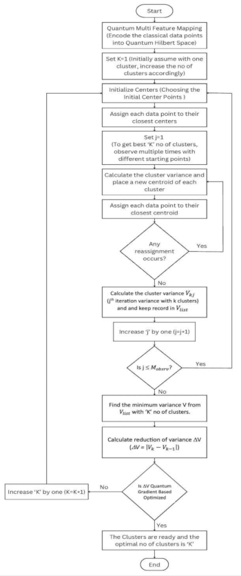
Figure 6: Flowchart of the proposed Hybrid Quantum K-Means Clustering procedure, showing quantum feature mapping, centroid initialization, iterative cluster assignment, quantum variance computation, variance-based convergence checking, and quantum gradient–assisted selection of the optimal number of clusters. Please click here to view a larger version of this figure.

The following steps outline the Quantum K-Means Algorithm for clustering cancer and non-cancer gene expression data.

Algorithm: Clustering Gene Expression Data of Cancer and Non-Cancer Cells Using the Quantum K-Means Algorithm

Step 1: Quantum Feature Mapping (Multi Feature Encoding).
Step 2: Assuming that initially all data points are belonging to the same cluster, so set the value of K=1 (Where, K: is the no of Optimal Clusters, V: is the Cluster Variance and ΔV: Reduction in Variance).
Step 3: Initialize Centers (Choosing the Initial Center Points using probability proportion of distances between the data points).
Step 4: Assign each data point to their closest centroid, which will form the predefined ‘K’ clusters.
Step 5: Calculate the cluster variance and place a new centroid of each cluster.
Step 6: Repeat the Step-4, which means reassign each datapoint to the new closest centroid of each cluster.
Step 7: If any reassignment occurs, then go to Step-5 else go to Step-8.
Step 8: Now we got the cluster C_j (‘j’th iteration with ‘k’ no of clusters) and calculate variance V_kj= , where ‘x’: data point belongs to the cluster C_i, and C_ci: cluster centroid of cluster C_i. Keep record of the variance V_kj in V_list and start again clustering with new Centers from Step 3 (Few no of times, i.e ‘j’ times, where 1 ≤ j ≤ M_obsrv) with same ‘K’.
Step 9: Find the minimum variance V from V_list with ‘K’ no of clusters.
Step 10: Calculate ΔV (ΔV = |V_k - V_k-1|, where V_k: is the variance with ‘K’ no of clusters and V_k-1: is the variance with ‘K-1’ no of clusters), if ΔV is Quantum Gradient Based Optimized (huge reduction) then FINISH else increase K (K=K+1) and goto Step 3 with new ‘K’.
Step 11: The Clusters are ready and the optimal no of clusters is ‘K’.

Quantum Features Mapping Algorithm

Algorithm 1: Quantum Features Mapping

Inputs: P points each of the quantum states |ψ〉 and |Φ〉
Output: An estimate of | 〈 ψ | Φ〉 |²
Algorithm Steps:
Step 1: We take a qubit and initialized it by zero; apply Hadamard gate and rotate it from Z basis to X-axis.
Step 2: We set ϕ (0 ≤ ϕ ≤ π ) in radian according on value of data point respect to feature 1.
ϕ = 2*rad(cos^-1)(d₀)),where d₀ represent the data values of feature 1 and d₀ ∈ [0, 1].
Step 3: We set θ (0 ≤ θ ≤ π ) in radian according on value of data point respect to feature 2.
θ = 2 * rad(cos^-1(d₁)), where d₁ represent the data values of feature 2 and d₁ ∈ [0, 1].
Step 4: We use the U3 quantum gate to implement the rotations performing encoding the features of data points.

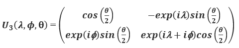
This rotates qubit Φ radian respect to positive x-axis and θ radian respect to positive z-axis.

Comparing Quantum States Algorithm

Algorithm 2: Comparing Quantum States

Inputs: Two qubit |q₁〉 and |q₂〉 each of the quantum states |ψ〉 and |Φ〉
Output: An estimate of | 〈ψ|Φ〉 |²
Algorithm Steps:
Step 1: Considering qubit A as ancilla and initialize it by state |0〉
Step 2: Apply Hadamard gate on the qubit A
Step 3: Apply CSWAP on the |q₁ 〉 and |q₂ 〉 qubit (on state|ψ〉 and |Φ〉), with A as the control qubit
Step 4: Apply Hadamard gate on the qubit A
Step 5: Measure A in on the basis of Z and record the measurement result as M
return M as our estimate of | 〈 ψ|Φ 〉 |²

Quantum-Distance-Estimator-for-k-means-clustering Algorithm

Algorithm 3: Quantum Distance Estimator and Choose new Cluster Centroid

Inputs: P no of datapoints and K no of cluster centroids, each of the quantum states |ψ〉 and |Φ〉
Output: New clustered centroid associated with the data points
Algorithm Steps:
for i in ranging from 1 to P:
Pick i^th data point and record it on |q_i 〉
for j in ranging 1 to K:
Pick j^th clustered centroid and set it on |q_j 〉
Compare Quantum States |q_i 〉 and |q_j 〉 i.e i^th qubit with j^th centroid and record the measurement in M as (M_i, j)
end for
Find the minimum distance (M_min ,min) from M and set min is the new centroid of |q_i 〉 and record it as C_i
end for
return C as our new centroid list

M= list of all clustered centroid distance from |q_i 〉 ith qubit
C = list of all newly computed minimal distance clustered centroid C_i of |q_i 〉; ∀_{(i∈{1,...,P})}

Initial Centroid Selection Algorithm

Algorithm 4: Calculate initial centroid points using probability proportion of distances between the data points

Inputs: m no of datapoints (X₁, X₂,...,X_m), each of the quantum states |ψ〉 and |Φ〉
Output: return a set S with K initial centroids
Algorithm Steps:
Step 1: Choose one point X randomly from data points X_i (1 ≤ i ≤ m) and add it to the set S
Step 2: For all X_i, calculate the distance between X_i using Quantum Distance Estimator and the nearest centroid point in S and set the distance as D_dist(X_i)
Step 3: Choose a number Y uniformly between 0 and D_dist(X₁)² + D_dist (X₂)² + ...+ D_dist (X_m)²
Step 4: Find a unique integer i such that
D_dist (X₁)² + D_dist (X₂)² + ...+ D_dist (X_i)² >= Y > D_dist (X₁)² + D_dist (X₂)² + ...+ D_dist (X_i-1)²
Step 5: Add X_i to S
Step 6: Until K centroids are found repeat Steps 2 – 4

return S as the initial centroid points

Quantum Variance Calculation Algorithm

Algorithm 5: Calculate Quantum Variance

Inputs: P no of datapoints, each of the quantum states | ψ〉 and |Φ〉
Output: return the variance of the data points
Algorithm Steps:
totalVariance ← 0
for i in ranging from 1 to K:
Pick i^th clustered centroid and set it on |q_i 〉
totalVariancei ← 0, M ← 0
for all j ∈ P, associated with cluster centroid i:
Pick j^th data point and set it on |q_j 〉
Compare Quantum States |q_i 〉 and |q_j 〉 i.e i^th centroid with j^th data point and record the measurement in M_j
M ← M + Mj
end for
totalVariance_i ← [C_i is the i^th cluster; |C_i | is no of data points in i^th cluster, D_k is the data point ∈ C_i & M_k
is distance between the centroid of C_i to D_k]
totalVariance ← totalVariance + totalVariancei
end for
return totalVariance

Quantum Gradient Based Optimization Algorithm (Getting Optimal no of Clusters)

The quantum gradient-based optimization step determines the optimal number of clusters by monitoring how intra-cluster variance changes as K increases. Compute the variance for consecutive values of K and evaluate the change between them. When the reduction in variance falls below the predefined threshold, additional clusters no longer improve compactness, and the corresponding K is selected as optimal. This curvature-based criterion ensures that clustering stops at the point where natural structure in the data is captured without over-partitioning.

Algorithm 6: Quantum Gradient Based Optimization

Inputs:
A parameterized quantum circuit QC(θ) with a single qubit rotation gate R_Y(θ).
A quantum observable  = Z (Pauli-Z expectation value).
A range of parameter values θ.
Output: The second derivative f′′(θ) of the expectation value 〈Z〉 with respect to θ.
Algorithm Steps:
Step 1: Initialize a single-qubit quantum circuit QC(θ) with:
A parameterized rotation gate R_Y(θ).
Measurement in the computational (Z) basis.
Step 2: Define the function Evaluate_ Expectation(θ) i.e. f′(θ) =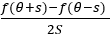
Bind the parameter θ to the circuit.
Execute the circuit on a quantum simulator with N shots.
Measure outcome probabilities P(0) and P(1).
Compute expectation value:
f(θ)=P(0)−P(1)
Step 3: Compute the Second Derivative using the Parameter-Shift Rule:
Set the shift value s =
Compute expectation values at shifted points:
f(θ+s), f(θ), f(θ−s)
Compute the second derivative:
f ′′(θ) =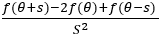
Step 4: f ′′(θ) to analyze variance reduction behavior.

The implementation details of the proposed quantum clustering approach are provided in Table 2. The table specifies the runnable functions and APIs used at each stage of the algorithm, including feature encoding into quantum circuits, execution of the SWAP test for distance estimation, centroid initialization, iterative cluster reassignment, and variance/ΔV evaluation. Circuit execution parameters, such as the use of SamplerV2 with the AerSimulator backend at 1024 shots and transpilation optimization level 1, are also listed. Furthermore, the table outlines the visualization methods applied to generate PCA scatterplots, variance plots, and histograms, as well as the clustering evaluation metrics (silhouette_score, calinski_harabasz_score, and davies_bouldin_score). By detailing specific command-level functions and APIs, the table ensures reproducibility of all computational steps in the proposed algorithm.

Results

A good cluster will depend upon various no of factors like, separation distance between clusters, within cluster distance, variance ratio criterion etc. So, Clustering performance was evaluated using three standard indices: the Silhouette Score, the Calinski-Harabasz Index (CH Index), and the Davies-Bouldin Index (DB Index). The Silhouette Score measures separation between clusters as

Discussion

This study proposes a novel Hybrid Quantum K-Means Clustering Algorithm with Optimal Cluster Detection, specifically designed to classify cancerous and non-cancerous samples using high-dimensional gene expression data. The approach integrates Quantum Multi-Feature Mapping, Swap Test-based quantum distance estimation, and Quantum Gradient-Based Optimization to dynamically determine the optimal number of clusters. Unlike traditional K-Means algorithms, which require a predefined number of cluster...

Materials

List of materials used in this article

Name	Company	Catalog Number	Comments
Apple MacBook Pro (M1 chip)	Apple Inc.	-	8?core CPU / 8?core GPU, 16?GB unified memory — used for local simulation
Breast Cancer Gene Expression Dataset	Kaggle	-	Dataset with 569 samples, 32 features (reduced via PCA in study)
macOS Monterey (Operating System)	Apple Inc.	12.6.9	Runtime environment used on local machine
math (Python standard library)	Python Software Foundation	built-in	Basic mathematical functions
Matplotlib	Matplotlib community	3.8.4	Plotting and visualization
NoiseModel, QuantumError, ReadoutError (Qiskit Aer)	IBM / Qiskit project	part of Aer 0.13.3	Used to simulate realistic quantum noise
NumPy	NumPy developers	1.26.4	Numerical operations and array manipulation
pandas	pandas development team	2.2.2	Data handling, I/O, tabular operations
Python	Python Software Foundation	3.10.12	Programming language, used in Jupyter / IPython environment
Qiskit Aer	IBM / Qiskit project	0.13.3	Simulator backend, with noise modeling and execution
Qiskit IBM Runtime – Session, SamplerV2	IBM / Qiskit project	0.41.1	Execution framework for circuits in simulator
Qiskit Terra	IBM / Qiskit project	0.45.0	Quantum framework for circuit construction and transpilation
scikit-learn	scikit-learn developers	1.4.2	PCA, clustering metrics, data preprocessing

References

- Mehta, V., Agarwal, M., Kaliyar, R. K. A comprehensive and analytical review of text clustering techniques. Int. J. Data Sci. Anal. 18 (3), 239-258 (2024).
- Bezdek, J. C. Pattern recognition with fuzzy objective function algorithms. , Springer Science & Business Media. (2013).
- MacQueen, J. Classification and analysis of multivariate observations. 5th Berkeley Symposium on Mathematical Statistics and Probability, , Univ. California. 281-297 (1967).
- Ester, M., Kriegel, H. P., Sander, J., Xu, X. A density-based algorithm for discovering clusters in large spatial databases with noise. KDD, 96 (34), 226-231 (1996).
- Roy, S., Bhattacharyya, D. K. An approach to find embedded clusters using density based techniques. Distributed Computing and Internet Technology (ICDCIT 2005), , Springer. 523-535 (2005).
- Guha, S., Rastogi, R., Shim, K. CURE: An efficient clustering algorithm for large databases. ACM SIGMOD Rec. 27 (2), 73-84 (1998).
- Zhang, T., Ramakrishnan, R., Livny, M. BIRCH: An efficient data clustering method for very large databases. ACM SIGMOD Rec. 25 (2), 103-114 (1996).
- Agrawal, R., Gehrke, J., Gunopulos, D., Raghavan, P. Automatic subspace clustering of high dimensional data for data mining applications. Proc. 1998 ACM SIGMOD Int. Conf. Management of Data, , 94-105 (1998).
- Wang, W., Yang, J., Muntz, R. STING: A statistical information grid approach to spatial data mining. VLDB, 97, 186-195 (1997).
- Theodoridis, S., Koutroumbas, K. Pattern recognition. , Elsevier. (2006).
- Mitsuda, N., et al. Approximate complex amplitude encoding algorithm and its application to data classification problems. Phys. Rev. A. 109 (5), 052423(2024).
- Horn, D., Gottlieb, A. Algorithm for data clustering in pattern recognition problems based on quantum mechanics. Phys. Rev. Lett. 88 (1), 018702(2001).
- Von Luxburg, U. A tutorial on spectral clustering. Stat. Comput. 17 (4), 395-416 (2007).
- Schölkopf, B., Smola, A., Müller, K. R. Nonlinear component analysis as a kernel eigenvalue problem. Neural Comput. 10 (5), 1299-1319 (1998).
- Schuld, M., Sinayskiy, I., Petruccione, F. An introduction to quantum machine learning. Contemp. Phys. 56 (2), 172-185 (2015).
- Schuld, M., Killoran, N. Quantum machine learning in feature Hilbert spaces. Phys. Rev. Lett. 122 (4), 040504(2019).
- Lloyd, S., Schuld, M., Ijaz, A., Izaac, J., Killoran, N. Quantum embeddings for machine learning. arXiv preprint. arXiv:2001.03622, (2020).
- Shao, J., Ahmadi, Z., Kramer, S. Prototype-based learning on concept-drifting data streams. Proc. 20th ACM SIGKDD Int. Conf. Knowledge Discovery and Data Mining, , 412-421 (2014).
- Lloyd, S., Mohseni, M., Rebentrost, P. Quantum algorithms for supervised and unsupervised machine learning. arXiv preprint. arXiv:1307.0411, (2013).
- Arthur, D., Vassilvitskii, S. K-means++: The advantages of careful seeding. Proc. 18th Annual ACM-SIAM Symp. Discrete Algorithms, , 1027-1035 (2007).
- Havlíček, V., et al. Supervised learning with quantum-enhanced feature spaces. Nature. 567 (7747), 209-212 (2019).
- Qi, J., Yang, C. H., Chen, S. Y. C., Chen, P. Y. Quantum machine learning: An interplay between quantum computing and machine learning. arXiv preprint. arXiv:2411.09403, (2024).
- Kang, M. S., Heo, J., Choi, S. G., Moon, S., Han, S. W. Implementation of SWAP test for two unknown states in photons via cross-Kerr nonlinearities under decoherence effect. Sci. Rep. 9 (1), 6167(2019).
- Barnett, S. M., Chefles, A., Jex, I. Comparison of two unknown pure quantum states. Phys. Lett. A. 307 (4), 189-195 (2003).
- Andersson, E., Curty, M., Jex, I. Experimentally realizable quantum comparison of coherent states and its applications. Phys. Rev. A. 74 (2), 022304(2006).
- Filippov, S. N., Ziman, M. Probability¬based comparison of quantum states. Phys. Rev. A. 85 (6), 062301(2012).
- Barenco, A., et al. Stabilization of quantum computations by symmetrization. SIAM J. Comput. 26 (5), 1541-1557 (1997).
- Buhrman, H., Cleve, R., Watrous, J., De Wolf, R. Quantum fingerprinting. Phys. Rev. Lett. 87 (16), 167902(2001).
- De Wolf, R. Quantum computing: Lecture notes. arXiv preprint. arXiv:1907.09415, (2019).
- Mashatola, L., Kader, Z., Abdulla, N., Kaur, M. Enhancing the Vietoris-Rips simplicial complex for topological data analysis: Applications in cancer gene expression datasets. Int. J. Data Sci. Anal. , 1-18 (2024).
Access restricted. Please log in or start a trial to view this content.