Ensemble of Temporal Weighting, Causal Inference, and Hierarchical Attribution towards SHAP Optimization

Summary

This article aims to assess the impact of temporal weighting, causal inference, and hierarchical attribution on interpretability optimization.

Abstract

During the past few years, the need for transparency and interpretability has been intensified owing to significant advancements in data-driven models, leading to the emergence of Explainable Artificial Intelligence (XAI). Several traditional XAI approaches are prevalent; however, these have limited competence in interpreting dynamic relations. The current research aims to address this limitation by proposing a novel Ensemble SHapley Additive exPlanations (SHAP) framework that focuses on temporal weighting, causal inference, hierarchical attribution, and interpretability optimization referred to as TCHSHAP. TCHSHAP prioritizes current information over historical information by temporal weighting through exponential decay. Further, causal inference separates correlation from causality to gain practical insights. Additionally, hierarchical attribution allows insights at granular (region level) and aggregated levels (feature-group impacts). These approaches are integrated to achieve a more interpretable and explainable model. To validate the efficacy of the proposed model, we carry out an experiment on the crop yield dataset collected from Kaggle. Ahead of experimental evaluation, data preprocessing is performed using one-hot encoding. Data normalization is done by min-max scaling, and outliers are removed through the Interquartile range. For the sake of experimental evaluation, the authors used the SHAP XAI model for Random Forest. When assessing the efficacy of the proposed TCHSHAP model, it is observed that while the average prediction for traditional SHAP is 161.137, it escalates to 161.506 after incorporating temporal weighting and causal inference, advocating the effectiveness of employing temporal and causal significance. Additionally, during hierarchical attribution, it is observed that agricultural features have the strongest dominance over the target variable. This dominance is followed by geographical and environmental factors in order. Thus, the obtained results authorize the efficacy of the proposed approach towards enhancing the global and local interpretability, strengthening the user's trust in model predictions. The current work offers ways to improve transparency and interpretability without affecting model performance. The suggested model also enables interpretable and efficient regression modelling in complex, data-driven applications, enabling its widespread application in real-world settings.

Introduction

Regression plays a major role in predictive analytics, encompassing several domains including climate modelling, financial forecasting, healthcare diagnostics, and agricultural yield estimation^1,2. However, the unexplained results of regression models, especially non-linear and high-capacity models like Gradient Boosting Machines (GBMs), Random Forests, and Deep Neural Networks (DNNs), pose significant challenges, particularly for applications requiring transparency and actionable insights. This interpretability gap can be bridged by employing Explainable Artificial Intelligence (XAI), a technique that is still in its infancy. Currently, conventional XAI frameworks like SHAP and Local Interpretable Model Agnostic Explanation (LIME) give only static feature explanations³. These XAI techniques presently fail to explain the intricacies of regression tasks involving temporal dependencies, hierarchical feature structures, and causalities, creating an avenue of research^4,5. Due to the non-consideration of these factors, XAI may sometimes derive incorrect conclusions. For instance, traditional SHAP only considers the correlation of attributes with the target variable without considering the causality. Let us consider a dataset with two input binary features, namely tobacco consumption and stained teeth. The target variable in this dataset is the probability of cancer. In such a scenario, if correlation is obtained between input features and the target variable, cancer will be highly correlated with both features (tobacco consumption and stained teeth). Now it is quite misleading to conclude that stained teeth cause cancer, as it is caused by regular tobacco consumption. Thus, it can be summarized that despite significant progress in the domain of XAI, the prime issues that need to be addressed in regression contexts include:

Inability to consider temporal dependencies leads to only static explanations that may not work in contexts with dynamic data.

Non-inclusion of causal inference in traditional SHAP adaptations causes false correlations rather than valuable causal insights.

Lack of attention towards hierarchical interpretation leads to insufficient higher-level aggregated explanations.

In order to address these issues, current research work aims to propose a novel XAI framework, TCHSHAP, that encompasses temporal weighting, causal inference, and hierarchical attribution with an aim to enhance the interpretability and computational efficiency of current XAI models. For the same, the proposed framework considers a temporal weighting factor w_t which assigns higher weights to the recent feature contribution in comparison to past values. This weighting factor aims to ensure that the interpretability aligns with the temporal significance of crucial features in dynamic regression problems such as yield forecasting and sales prediction. Further, traditional regression models fail to exhibit causal relationships, leading to ambiguous attributions⁶. To address this challenge, the proposed framework adopts Structural Causal Models (SCMs) to assess the causal impact of a feature F_i on the output. Additionally, the real-time datasets often demonstrate hierarchical relations (spatial or categorical) among features, which are seldom showcased in existing XAI frameworks^4,5,6. On the contrary, the suggested XAI framework aggregates individual features (F_i) to obtain higher-level features (H_j), to achieve granularity of the explanations.

Apart from incorporating temporal, causal, and hierarchical significance, the proposed ensemble also aims to enhance interpretability and explainability. Such an objective is an effort towards establishing the trade-off between interpretability and accuracy, ensuring that the explanations obtained from TCHSHAP are accurate and interpretable⁴. The suggested XAI framework can be mathematically described as follows, while the description of the used variables is given in Table 1. The traditional SHAP value for the feature is calculated as equation (1)^5,6.

   (1)

This traditional SHAP formulation adds up contributions without considering temporal, causal, or hierarchical adjustments.

Variable	Definition
Fi	Feature whose Shap value is being calculated
Shapi	Shap value of the Feature
S	Set of total Features
M	Subset of all features
FT	Total number of Features
P(M)	Model Prediction when only features in M are used
λ > 0	decay rate
T	Reference Prediction Time
Y	Output

Table 1: Description of variables used. This table describes the significance of various variables used.

This traditional SHAP formulation is modified to handle dynamic dependencies by including temporal weighting. This temporal weighting is incorporated by introducing the weighting coefficient wt = e^{-λ |t - T|} where λ represents decay factor (λ > 0) . As discussed earlier, this exponential weighting gives more weight to recent values compared to past values. This exponential decay is included with an understanding that recent feature values have higher significance than past values. The modified SHAP value (after incorporating temporal significance) is given in equation (2).

  (2)

This temporal information is important for dynamic regression tasks like predicting yields or stocks.

Further, in order to make the explanations more robust, SCM is applied to assess the causal impact of the feature F_i on the output Y. The mathematical formulation for causal SHAP is given in equation (3)

 (3)

Here do(F_i) represents the feature that has contributed to the change. By using this, the model achieves the competence to explain the causality rather than the correlation. It is worth noting that SCM-based computation of causal effects ensures that only features with direct causal influence are given credit, eliminating false correlations.

Further, the hierarchy is proposed in the suggested model to aggregate attributes across various levels. The mathematical formulation for the hierarchical SHAP is given in equation (4).

  (4)

Incorporation of hierarchy in the suggested model ensures the achievement of granularity of the explanations. The suggested framework is depicted in Figure 1.

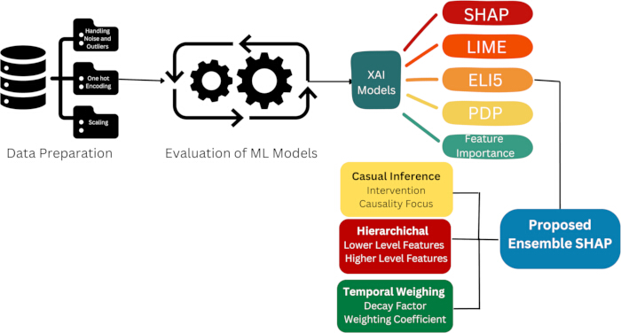
Figure 1: Pictorial illustration of various elements in the proposed framework. This figure gives a pictorial illustration of various elements in the proposed framework TCHSHAP that include temporal weighting, causal inference, and hierarchical attribution. Please click here to view a larger version of this figure.

The novelty of the proposed model TCHSHAP lies in handling these three inconsistencies by employing temporal weighting (to give more weight to current information), Structural Causal Models (SCM; to assess causal effects), and hierarchical aggregation of SHAP values (to gain multi-level insights). Thus, the proposed ensemble expands SHAP beyond its static constraints, providing a regression-optimized explanatory framework.

Proposed TCHSHAP has the potential to achieve great significance for real-time applications in scenarios requiring better decision-making, as it identifies the detailed explanations of the output in regression models, seamlessly connecting modelling with decision-making. In summary, the prime contribution of this manuscript is to design a novel framework that combines temporal weighting, causal inference, and hierarchical relations to enhance the actionable explanations of the traditional SHAP model.

Related work

XAI incorporates different methodologies specially designed for enhancing the transparency and interpretability of different machine learning models. These XAI strategies establish confidence in the results by providing the required insights from the results. For instance, notable XAI methodologies such as LIME and SHAP enhance the interpretability and transparency of otherwise black box models across various domains, namely finance, education, and the healthcare sector⁷. Also, XAI techniques are applied in tasks related to software analytics, clone detection, and Just-in-Time defect prediction⁸. Additionally, Awal and Roy also highlighted the discrepancies and demonstrated lesser reliability in generating the explanations⁸. Here, the authors applied Granular Level Evaluation Metrics for reducing consistency in evaluation. XAI has also been widely employed in the medical domain to understand the most prominent factors affecting the results of the classification task and hence fostering the faith among health practitioners to use AI-based diagnostics^9,10,11,12. Further, in sectors like Belgian residential rent prediction, XAI approaches facilitate the interpretation of intricate models, hence enhancing quality control and minimizing production errors¹³. Bommer et al. demonstrated that integration of XAI methods with gradients enhances the performance of XAI methods in terms of robustness, faithfulness, complexity, and randomization in climate science¹⁴. A lot of researchers have attempted to create ensemble and hybrid techniques. In addition to proposing ensemble techniques, researchers also demonstrated the effectiveness of these hybrid techniques towards providing comprehensive insight for complex models^15,16. A detailed review of the techniques, optimizations, and the various applications are tabulated in Table 2, which clearly indicates that the most widely applied techniques are LIME and SHAP. The future research direction points towards exploring optimization in these methods to enhance the interpretability of these models. Continuing the line of research, authors in current research work focus on SHAP optimization by adding causal inference, hierarchical attribution, and temporal weighting.

Citation	XAI Techniques	Optimization	Insights	Applications	Future Research Directions
(Anushree et al., 2024)	LIME	Not provided	Enhancement of interpretability and transparency of black box models across various applications in Finance, education and healthcare sector.	· Trade-off between Accuracy and Interpretability in Finance, Education and healthcare sector	· Need to develop a list of detailed metrics for evaluating various XAI models
	SHAP
	Perturbation mechanisms
	Attention-based mechanisms
(Awal & Roy, 2024)	PyExplainer	Granular Level Evaluation Metrics for reducing consistency in evaluation.	Highlights the discrepancies and demonstrates lesser reliability in generating the explanations.	· Tasks related to Software Analytics	· Advance research methods are required for enhancing the reliability of XAI models for tasks related to software analytics
	LIME			· clone detection
				· Just in Time Defect Prediction
(Bommer et al., 2024)	Integrated Gradients	Integration of XAI methods with Gradients	Integration of XAI methods with gradients enhances the performance in terms of robustness, faithfulness, complexity, and randomization in climate science.	· Climate Science Prediction	· Focus on task specific evaluation of climate science.
	layer-wise relevance propagation			· Annual mean Temperature maps prediction
	input times gradients
	sensitivity methods like gradient, SmoothGrad, NoiseGrad, and FusionGrad
(Bhatnagar & Agrawal, 2024)	LIME	Ensemble of XAI Techniques	Ensemble provides comprehensive insight and enhance interpretability and explainability of complex models.	· Applied on Moral dataset to enhance the interpretability of the results	· Explore hybrid XAI methods by combining multiple techniques
	SHAP				· Customizing various XAI algorithms for specific models catering to different needs of the users
(Dias, 2024)	LIME	Integration of XAI Techniques	Improved Interpretability and Accuracy	· Toxic Comment Classification	· Enhancing the strength for classification purpose.
	Eli5
(Hajare et al. ,2024)	SHAP	Not Provided	SHAP offers detailed insights into the risk factors in predicting the Acute Coronary Syndrome.	· Acute Coronary Syndrome (ACS)	· To find out novel risk factors in ACS prediction.
(Hamida et al., 2024)	Comprehensive review of various XAI Techniques	Not Provided	Provides insights on XAI applications XAI in the healthcare sector emphasizing the importance of explainability of AI decisions to understand the results provides by AI.	· Actionable Insights in Healthcare sector	· Enhancement of XAI components namely comprehensibility, transparency, interpretability, and explainability.
					· Custom XAI techniques for healthcare sector for detail insights for healthcare domain
(Ihongbe et al., 2024)	Grad-CAM (Gradient-weighted Class Activation Mapping)	Gradient-weighted Class Activation Mapping	Better accuracy for Pneumonia and COVID-19 diagnosis.	· Improved Accuracy for medical diagnosis	To increase the awareness of the usability of XAI techniques for real life applications
(Lenaers, & De Moor, 2023).	6 XAI Techniques	Ensemble of 6 XAI Techniques on CatBoost Model	Multiple techniques enhance the interpretability of XAI for rent prediction.	· Belgian residential rent prediction	XAI can be utilized for decision making
(Makumbura et al., 2024)	SHAP	Ensemble of RF, LightGBM, XGBoost with SHAP	SHAP reveals the various factors responsible for assessing and predicting the water quality.	· Assessment and prediction of water quality	Can be employed for decision making
(Schlegel & Keim, 2023).	XAI Techniques with Perturbation Analysis	Perturbation Analysis	Can be effectively employed for classification tasks of Time Series Data	· Time Series Data of Finance, Healthcare, Climate science	To combine multiple XAI techniques for enhanced interpretability.
(Silva & Keller, 2023)	XAI	Not Provided	XAI models have a limitation to explain the results in case of correlated features. Can be employed for Earth and atmospheric sciences.	· Atmospheric sciences	XAI need to be optimized for correlated features to avoid false explanations.
	Biomolecular Reaction Rate			· Atmospheric Chemistry
(Y, S., & Challa, M. 2023)	SHAP	Not Provided	Here, XAI models are compared with respect to interpretability and understanding important features and concluded that SHAP and LIME are the most effective.	· Medical Applications	To enhance interpretability for advanced medical applications
	LIME
	PDP
	GAM

Table 2: Comprehensive review of various optimizations done on XAI techniques. This table presents a comprehensive review of different optimization techniques suggested by various researchers.

Protocol

NOTE: This section discusses the proposed ensemble method, including all the proposed amendments as illustrated in Figure 1.

Data preparation

In order to validate the effectiveness of the proposed framework, the authors carried out an experiment on the crop yield dataset collected from Kaggle¹⁷. This dataset consists of Indian agricultural data for various crops from 1997 to 2020 and was accessed in March 2025. This dataset comprises numerous features, namely season, crop_year, fertilizer, pesticide, crop, and yield (target variable), etc. The considered dataset is pre-processed for enhanced efficiency using one-hot encoding to handle categorical values. The categorical features like season, crop, and state are one-hot encoded. MinMax scaling is also employed to scale the numerical features such as area, production, annual_rainfall, fertilizer, and pesticide to the [0,1] range. In order to handle the outliers, we used the Interquartile Range rule with a threshold Q₁ - 1.5 • IQR¹⁷. A random seed of 42 was applied across all preprocessing steps in order to get the reproducibility of the results. Further, the dataset was split into a training (80%) and a testing dataset (20%) after preprocessing.

Experimental setup

The experiment was carried out using Python 3.10 on an A100 GPU Server with CPU: Dual AMD Rome 7742, 128 cores, 1TB RAM. Libraries imported for simulation are scikit-learn 1.3.0, XGBoost 1.7.6, TensorFlow 2.13, SHAP 0.41.0, LIME 0.2.0.1, and ELI5 0.13.0.

Evaluation of ML models

Here, authors have used various regression models namely LinearRegression(), Ridge(alpha=1,random_state=42), Lasso(alpha=0.1,random_state = 42), Decision TreeRegressor(max_depth = 10, random_state = 42), RandomForestRegressor(max_depth = 15random_state = 42), GradientBoostingRegressor(n_estimators = 200, learning_rate = 0.1, random_state = 42),  XGBoost, and CNN to determine the impact of various variables on the target variable yield¹⁸. XGBoost uses 300 estimators and a learning rate of 0.05. In the CNN model, two hidden layers, ReLU activations, and Adam optimizer are used with a learning rate of 0.001. The efficiency of these models is compared using different performance metrics. These models also perform hyperparameter tuning. For instance, Ridge regression and Lasso regression are trained with alpha equals 1.0 and alpha equals 0.1, respectively. In Decision Tree and Random Forest, the maximum depth was set to 10 and 15, respectively. Gradient Boosting uses 200 estimators and a learning rate of 0.1. The performance of these models was evaluated using 5-fold cross-validation in terms of Mean Squared Error (MSE) and R2 square.

Evaluation of XAI models

As discussed, the current work uses various XAI models to compare the results. Here, the authors use shap.TreeExplainer(model,data = crop_yield) for tree-based models (Random Forest, Gradient Boosting, and XGBoost). A background dataset of 100 randomly selected cases was chosen from the training dataset to stabilize attributions. Further, shap.KernelExplainer()  was used for non-tree models (Linear, Ridge, Lasso, and CNN) with 1000 perturbations to get close to SHAP values. Tabular explainer (lime.lime_tabular.LimeTabularExplainer) was used with 5000 perturbations per instance to run LIME on the same background dataset to ensure that local explanations are stable. The kernel width was set based on characteristics, and the model's prediction function was used to infer explanations. Local explanations were generated by calling explainer.explain_instance(x,model.predict). ELI5 was utilized as permutation importance with 10 repetitions on the validation split to avoid overfitting of the test data, and was simulated using eli5.sklearn.PermutationImportance(estimator,random_state = 42). The significance of mean and variance among repeats was exhibited during the experiment. Finally, the fitted model was used for the validation split to obtain Partial Dependence Plots (PDPs), which were implemented using PartialDependencyDisplay.from_estimator (model,X_val,features = [feature]),

Set up of the TCHSHAP framework

Subsequently, TCHSHAP was implemented by applying various steps in sequence. The first step in the sequence was temporal weighting that uses an exponential decay function with a decay rate of λ = 0.85, which was selected based on an ablation study across λ  [0.7.0.95]. The reference time (T_current) was selected as the recent crop year in the dataset. This ensures that the model explanations consider the dynamics of the agricultural output forecast, where recent features (rainfall, fertilizer use, or pesticide) carry more significance for making decisions. Temporal weighting was followed by SCM to adopt causal inferences. The suggested methodology uses the dot operator to simulate interventions and calculate the Average Causal Effect. The causal inference was applied using python doWhy 0.13 library. This helps to alleviate misleading connections due to correlated inputs like production and area, achieving real cause-and-effect links. The final step in the pipeline was hierarchical attribution, where features were organized into higher-level domains. For the current dataset, there are 3 hierarchical features, namely Agricultural Inputs (Fertiliser, Pesticide), Geographical Factors (State, Area, Crop_Year), and Environmental Factors (Annual_Rainfall, Season). By using normalised summation to group SHAP data, explanations at both levels (detailed and general) can be obtained.

In summary, the TCHSHAP pipeline combines three steps-temporal adjustment, causal attribution, and hierarchical grouping into a single process. Here, baseline SHAP first makes explanations, followed by the addition of three improvements. This structured pipeline ensures that TCHSHAP's outputs are consistent, can be reproduced, and give both local and global explanations. The step-by-step description of the proposed framework is given in the pseudocode below.

Input: 
X: Dataset with features X₁,X₂,X₃,........,X_n.
t: temporal variable in the dataset 
T_current: Reference time 
λ: Decay rate
G: Feature Groups
Compute Temporal Weights
For each instance, i X, evaluate w_t = e^-λ|t-T|,
Calculate Shap Values Shap_i
    Calculate Shap_Tempral = Shap_i * w_t
Compute Causal Inference
    For each Feature, X_i  X 
Calculate Shap_Causal = Shap_i * Causal Effect(X_j →Y)   
Hierarchical Attribution
    For each Feature, X_i  X 
Calculate Shap Values Shap_i
For each G_i  G

Output: Set of Hierarchically aggregated SHAP values 

The quantitative checkpoint for facilitating troubleshooting is given below: Random Forest yielding the lowest MSE and highest R² across all ML models. The feature importance obtained was Area > Pesticide > Fertilizer, with Season and Crop_Year as minimal. The global baseline SHAP prediction was 161.137. Further, after applying λ = 0.85, the contribution of Crop_year and Season increases. Group-level contributions follow the order Agricultural Inputs>Geographical Factors> Environmental Factors.

Results

This section discusses the results obtained by applying various methods used during the experiment study, comprising various subsections as follows:

Data collection and preprocessing

In order to perform an experimental evaluation of the proposed framework, a dataset regarding crop yield was collected from Kaggle¹⁹. The collected...

Discussion

The prime objective of the current study is to incorporate temporal weighting, causal inference, and hierarchical significance in the traditional SHAP model, yielding the TCHSHAP model. The motive behind including these components in XAI techniques is to enhance the interpretability of the results. For temporal weighting, we have considered an exponential decaying technique, which gives more weightage to recent values in comparison to old values. In causal significance, authors try to assess the direct impact of various ...

Materials

List of materials used in this article

Name	Company	Catalog Number	Comments
ELI5	0.13.0	PyPI
LIME	0.2.0.1	PyPI
Nvidia DGX A100 GPU Server	CPU Dual AMD Rome 7742, 128 cores total	Nvidia
System Memory 1TB
Python	3.1	Python
SHAP	0.41.0	PyPI
scikit-learn	1.3.0	PyPI
TensorFlow	2.13	Tensor Flow
XGBoost	1.7.6	PyPI

References

- Kaur, B., et al. N-Beats architecture for explainable forecasting of multi-dimensional poultry data. PloS One. 20 (4), e0320979(2025).
- Sharma, N., Mangla, M., Iqbal, M. M., Mohanty, S. N. Deep Learning Framework for Identification of Skin Lesions. EAI Endorsed Trans Perv Health Tech. 9, (2023).
- Sharma, N., Mohanty, S. N., Mahato, S., Pattanaik, C. R. A novel dataset and local interpretable model-agnostic explanations (LIME) for monkeypox prediction. Intell Decision Technol. 17 (4), 1297-1308 (2023).
- Makumbura, R. K., et al. Advancing Water Quality Assessment and Prediction Using Machine Learning Models, Coupled with Explainable Artificial Intelligence (XAI) Techniques Like Shapley Additive Explanations (SHAP) For Interpreting the Black-Box Nature. Results Eng. 23, 102831(2024).
- Schlegel, U., Keim, D. A. A Deep Dive into Perturbations as Evaluation Technique for Time Series XAI. Communic Comp Informat Sci. 1903, (2023).
- Silva, S. J., Keller, C. A. Limitations of XAI methods for process-level understanding in the atmospheric sciences. Artificial Intell Earth Syst. 3 (1), e230045(2024).
- Anushree, G., Madagaonkar, S. B., Ravili, C. H. Unveiling the Black Box: A Comprehensive Review of Explainable AI Techniques. Int J Sci Res Eng Manag. 8 (9), 1-11 (2024).
- Awal, M. A., Roy, C. K. EvaluateXAI: A framework to evaluate the reliability and consistency of rule-based XAI techniques for software analytics tasks. J Syst Software. 217, 112159(2024).
- Hajare, S. W., Rewatkar, R., Reddy, K. Design of an iterative method for enhanced early prediction of acute coronary syndrome using XAI analysis. AIMS Bioeng. 11 (3), 301-322 (2024).
- Hamida, S. U., Chowdhury, M. J. M., Chakraborty, N. R., Biswas, K., Sami, S. K. Exploring the landscape of explainable artificial intelligence (XAI): A systematic review of techniques and applications. Big Data Cognit Comput. 8 (11), 149(2024).
- Ihongbe, I. E., Fouad, S. F., Mahmoud, T., Rajasekaran, A., Bhatia, B. Evaluating Explainable Artificial Intelligence (XAI) techniques in chest radiology imaging through a human-centered Lens. PloS One. 19 (10), e0308758(2024).
- A Comparative Analysis of Explainable AI Techniques for Enhanced Model Interpretability. Swathi, Y., Challa, M. 3rd Int Conf Pervasive Comput Social Netw, , 229-234 (2023).
- Lenaers, I., De Moor, L. Exploring XAI techniques for enhancing model transparency and interpretability in real estate rent prediction: a comparative study. Finance Res Lett. 58 (Part A), 104306(2023).
- Bommer, P. L., Kretschmer, M., Hedström, A. K., Bareeva, D., Höhne, M. Finding the right XAI Method - A Guide for the Evaluation and Ranking of Explainable AI Methods in Climate Science. Artif Intell Earth Syst. 3, e230074(2024).
- Bhatnagar, S., Agrawal, R. Understanding explainable artificial intelligence techniques: a comparative analysis for practical application. Bullet Elect Eng Info. 13 (6), 4451-4455 (2024).
- Ennab, M., Mcheick, H. Enhancing interpretability and accuracy of AI models in healthcare: a comprehensive review on challenges and future directions. Front Robot AI. 11, 1444763(2024).
- Wan, X., Wang, W., Liu, J., Tong, T. Estimating the sample mean and standard deviation from the sample size, median, range and/or interquartile range. BMC Med Res Methodol. 14 (1), 135(2014).
- Mangla, M., Shinde, S. K., Mehta, V., Sharma, N., Mohanty, S. N. Handbook of Research on Machine Learning: Foundations and Applications. , CRC Press. (2022).
- Gupta, A. Agricultural Crop Yield in Indian States Dataset [Data set]. , Kaggle. https://www.kaggle.com/datasets/akshatgupta7/crop-yield-in-indian-states-dataset (2025).
- Shin, J., Miah, A. S. M., Konnai, S., Hoshitaka, S., Kim, P. Electromyography-Based Gesture Recognition with Explainable AI (XAI): Hierarchical Feature Extraction for Enhanced Spatial-Temporal Dynamics. IEEE Access. 13, 88930-88951 (2025).
- Das, A., Rad, P. Opportunities and challenges in explainable artificial intelligence (xai): A survey. arXiv. , (2020).
- Srinivasu, P. N., Sandhya, N., Jhaveri, R. H., Raut, R. From blackbox to explainable AI in healthcare: existing tools and case studies. Mobile Info Syst. 2022 (1), 8167821(2022).
- Fiok, K., Farahani, F. V., Karwowski, W., Ahram, T. Explainable artificial intelligence for education and training. J Defense Model Simulat. 19 (2), 133-144 (2022).
Access restricted. Please log in or start a trial to view this content.