A Novel Approach Using AI-vision Transformer for CT Scan Analysis for Lung Cancer Detection

Summary

The use of Vision Transformers in this study allows lung cancer to be classified from CT images, achieving an accuracy of 98.18%, at 1,190 scans. The model preserved a satisfactory level of robustness, with accuracy levels between (80–88%) with noisy and blurred images, against standard convolutional neural network (CNN) models, in consumer health diagnostic applications.

Abstract

Diagnosing lung cancer remains challenging because of the subtle differences between benign versus malignant disease on imaging studies. While traditional, convolutional neural networks (CNNs) have been the mainstay of medical imaging analysis, they still have limited applicability and robustness with variation of imaging methods. The advancement of machine learning is transforming traditional methods of diagnosis in consumer-facing healthcare technologies, changing processes in accessibility and personalized patient care. This paper describes the use of Vision Transformers (ViTs) for the task of lung cancer classification with CT scans, associated with consumer health applications. The Vision Transformer model was trained on complete dataset of 1,190 CT images, and achieved a classification rate of 98.18% with a Matthews Correlation Coefficient of 0.9676. Additionally, the model's performance was validated on simulated real-time scenarios using real-time noises and blurred datasets. Although preserving validation methods with strong diagnostic accuracy, across the entire dataset the ViT model also outperformed the conventional validated method by showing an accuracy of between 80-88% to differentiate between the noisy images and fuzzy images, even under these circumstances. While initial results provide promising information about the robustness of ViTs when dealing with image variation, a cautious approach should still be exercised in contextualizing results since the evaluation studies were completed within a relatively small dataset and simulation settings. It will be valuable for future research studies to use larger datasets that are more representative of true clinical conditions and datasets that are clinically validated to determine whether ViTs are advantageous to clinical identification of oncology diagnostic and to improve early detection.

Introduction

Lung cancer has a substantial global burden, affecting millions of lives every year. Due to the cancer's aggressive nature and frequent late-presenting disease state, the mortality associated with lung cancer is high. Early detection is essential because the intervention can improve treatment effectiveness and survival rates a great deal¹. The conventional approach for preliminary screening and diagnosis remains with the utilization of computed tomography (CT) to allow more detailed visualization of the pulmonary structures. However, the evaluation of the CT images is complex and is entirely dependent on the reviewers as radiologists. Tumor variability in attributes such as size, shape, and density also mitigate the reliability of any human observation. Environmental factors can challenge accuracy and reproducibility of decision making based on human analysis.
With these limiting factors in mind, recent literature has made a strong push for the application of artificial intelligence (AI) to medical imaging, with more focus on deep learning (DL) models. DL, especially with Convolutional Neural Networks (CNNs), have disrupted the pattern of observations in medical imaging by changing the analyses of images². CNNs have significantly enhanced diagnostic processes in oncology, demonstrating the ability to identify subtle and complex features in imaging data that are often indistinguishable to the human eye. Despite these advancements, CNNs face limitations overfitting on small datasets, reduced robustness under variable acquisition conditions, and reliance on local receptive fields that can miss global dependencies. While hybrid CNN-Transformer approaches attempt to combine convolutional priors with attention mechanisms, they still inherit biases of convolutional architectures. Figure 1 shows a few instances from the dataset showcasing different classes.

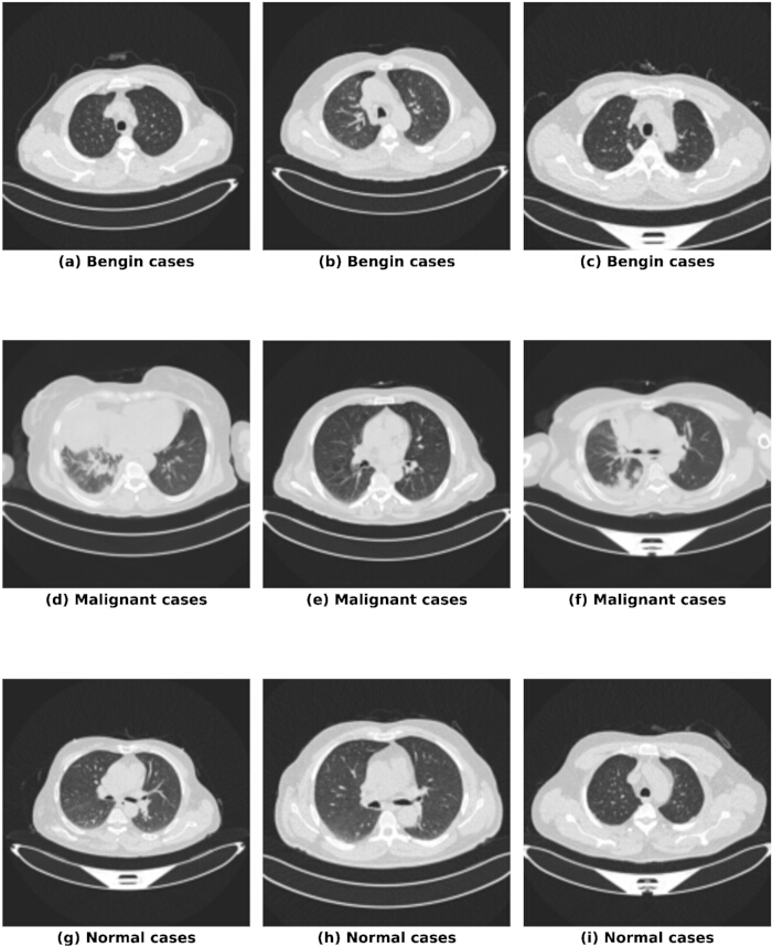
Figure 1: Visual illustration of different classes showing representative CT scan slices of normal, benign, and malignant lungs, highlighting their similarities and differences. Please click here to view a larger version of this figure.

Representative CT images are shown for normal, benign, and malignant cases. While explicit marking of discriminative regions would aid visual interpretation, manual annotation requires expert radiologists and was beyond the scope of this study. 

Vision Transformers (ViTs), originally introduced for natural image classification³, present a promising alternative. Unlike CNNs or CNN-Transformer hybrids, ViTs employ a fully attention-driven framework that captures global contextual information across an entire image. This study is especially pertinent for CT imaging, where the diffuse and irregular character of tumor attributes can extend throughout regions as opposed to being limited just to local receptive fields. While CNN-Transformer hybrid networks stabilize the convolutional inductive bias, Vision Transformers (ViTs) implement a completely attention-based architecture, allowing the ViT model to capture long-range dependencies across entire CT images - a benefit when assessing diffuse or irregular lung tumor attributes.

The advent of transformer-based models in the field of medical imaging is recent, with some examples in soft radiology and histopathology,^4,5,6 which have exhibited notable advantages for robustness to noise, blur, and inter-scanner variability than traditional CNN systems, in supporting a justification for ViT in such clinical context without overemphasizing novelty. Given a stricter approach to lung cancer imaging versus consumer - health applications, this study aims to justify practicality in a robust area of evidence-based medicine, while situating itself among the not altogether overwhelming literature recently available pertaining to transformers, and its applications. Previous literature has demonstrated that accuracies from CNN diagnostic modalities drop drastically due to acquisition variability⁷, where the corresponding ViT does better with the same perturbations,⁸ which gives credence to the concept of using a ViT in assessment modalities and presenting an option to increased reproducibility in diagnostic workflows. Moreover, practical issues, such as required dataset size, computational burden, and generalizability to different clinical settings are clearly levied in the study with the use of methods such as data augmentation, transfer learning, and efficient ViT variants^9,10 to address these potential challenges in real-world use. 

This study builds upon this advancement by implementing ViTs for lung cancer staging using CT image data and examining the robustness and generalizability of the model in the presence of real-world imaging problems. CT data has the potential to include artifacts, noise, and blurring to a common extent that may obscure features meaningful to clinicians. By examining resilience to these changes in imaging, this study aims to offer an additional staging framework capable of being relied upon in practice when making decisions related to care and treatment.

The contributions of this study involve: i) specifically detecting lung cancer from CT images in the IQ-OTH/NCCD dataset by using and examining the performance of a Vision Transformer model; ii) assessing how well the model performs in real-world clinical imaging scenarios common to CT data, such as noise and blurriness; iii) comparison of accuracy, sensitivity, and specificity of ViTs as an alternative to traditional CNN models.

The organization of the remainder of this paper is as follows: Section II goes through the literature review providing prior work related to lung cancer detection using deep learning techniques and the progression from CNNs to more advanced architectures such as the ViTs. Section III presents the approach taken for this work which includes data preprocessing, model architecture information and training procedure details. Section IV presents the findings specifically addressing the prescriptive features of ViTs as a clinical method and how it may enhance the accuracy and reliability of lung cancer screenings. Section V summarizes the findings and contributions to practice and discusses future directions in the context of deep learning in a medical environment.

RELATED WORK:

Deep learning (DL) has revolutionized medical imaging during the last ten years, especially in the diagnosis of lung cancer. At first, the discipline depended on conventional machine learning techniques like Support Vector Machines (SVMs) and decision trees, which were constrained by the need for well-built, properly obtained features. These features handled the intricacies of medical pictures poorly and often injected subjectivity.

A significant change was brought about with the invention of Convolutional Neural Networks (CNNs), which made it possible to automatically extract hierarchical characteristics from data¹¹. CNNs have been widely used in CT scan-based cancer staging, nodule detection, and classification as benign or malignant. CNNs are successful, but they have limitations. These include differences in image collection settings and the need for big, annotated datasets, which are hard to come by because of privacy issues and the labour-intensive nature of medical annotation. Table 1^{12,13,14,15,16,17,18,19,20} provides the summary of recent studies carried out in the field of lung cancer diagnosis.

Crasta, Lavina Jean, Rupal Neema, and Alwyn Roshan Pais (2024) [20]

To present a novel deep learning framework for lung cancer detection and classification using CT images [20].

The paper introduces a 3D-VNet for segmentation and a 3D-ResNet for classification, showcasing improvements in accuracy and robustness over previous methods.

Crasta, Lavina Jean, Rupal Neema, and Alwyn Roshan Pais (2024) [20]

To present a novel deep learning framework for lung cancer detection and classification using CT images [20].

The paper introduces a 3D-VNet for segmentation and a 3D-ResNet for classification, showcasing improvements in accuracy and robustness over previous methods.

Table 1: Summary of recent studies outlining techniques used and reported performance for context.

By using self-attention processes that consider an image's whole context at once, Vision Transformers (ViTs) are starting to emerge as a competitive alternative to CNNs in image-related tasks. ViTs are especially promising for medical imaging, because the significance of some regions may depend on farther-off portions of the picture due to their global processing capability. However, despite their capacity to handle complicated tasks like recognizing correlations between numerous illness indicators in scans, ViTs are still not well-studied in the medical imaging field.

ViTs have not been explored to a great extent in the field of the consumer-centric health care devices. This study aims to bridge the gap between high accuracy and less latency for consumer-centric health care devices where they can perform well and can give accurate predictions in the real-time.

Protocol

The dataset includes a total of 1,190 CT scan slices from 110 cases, categorized into three classes: normal (55 cases), benign (15 cases), and malignant (40 cases). Each case comprises multiple CT slices (ranging from approximately 80 to 200 slices per case), offering diverse axial views of the thoracic region. The CT images were obtained in DICOM using the SOMATOM scanner with standard imaging parameters: tube voltage = 120 kV, slice thickness = 1 mm, window width = 350–1,200 Hounsfield Units (HU), and window center values = 50–600 HU, during a full inspiration breath hold.

All images were fully de-identified prior to analysis to remove any personally identifiable information (PII). The dataset was ethically approved by the institutional review boards of the participating medical centers, with written consent waived by the oversight review board. The cases included individuals from varied backgrounds such as government employees, farmers, and residents from several Iraqi provinces (including Baghdad, Wasit, Diyala, Salahuddin, and Babylon) with diversity in gender, age, educational level, and living status.

As the dataset is publicly available and de-identified, no additional ethical approval was necessary for its use in this study. The dataset adheres to the terms and conditions specified by its original contributors and the hosting platform.

The methodology of this research uses a multi-stage process designed to create a prediction model with the help of the IQ-OTH/NCCD lung cancer dataset²¹. This methodology sets a strong stage for the consumer centric health care devices where less latency is required, which can give better accuracy. Figure 2 depicts the working mechanism of the proposed model.

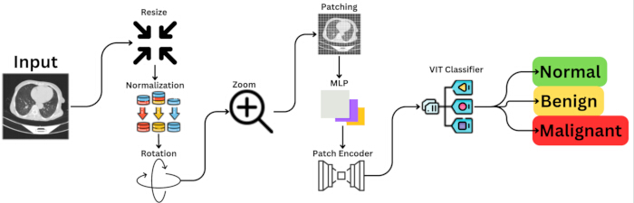
Figure 2: Workflow diagram of the proposed model depicting preprocessing, augmentation, Vision Transformer classification, and evaluation steps. Please click here to view a larger version of this figure.

1. Dataset description

The IQ-OTH/NCCD lung cancer dataset was collected at the Iraq-Oncology Teaching Hospital/National Center for Cancer Diseases during the fall of 2019. The training part of the dataset used contained 1,097 images whose description is given in Table 2, which illustrates the count of sample instances of different classes.

Class	Number of Images
Normal	416
Benign	120
Malignant	561

Table 2: Sample instances of normal, benign, and malignant CT images from the dataset.

The IQ-OTH/NCCD lung cancer dataset was chosen for its comprehensive representation of normal, benign, and malignant CT scans. While other datasets, such as LIDC-IDRI and NSCLC-Radiomics, are available, they either focus primarily on nodule detection or lack sufficient samples of benign cases. The IQ-OTH/NCCD dataset is particularly suitable for our study as it allows the Vision Transformer to learn discriminative features across all three classes, enabling robust classification of subtle patterns in lung CT images. 

2. Data preprocessing

Preprocessing is an important step in improving model performance through consistency and appropriate adjustments to the data that will be processed through the neural network. In order to ensure consistency in the input size for the neural network, we have scaled all images to the same dimension of 256 x 256 pixels, and normalized the data to a pixel value between 0 and 1 in the hopes to improve model training and convergence. Table 3 contains the augmentation technique values.

Technique	Value
Normalization	-
Resizing	image_size x image_size
RandomRotation	factor=0.02
RandomZoom	height_factor=0.2, width_factor=0.2

Table 3: Applied augmentation techniques with parameter ranges.

To increase the robustness of the model against overfitting and improve its ability to generalize, data augmentation techniques such as random rotations and zooms are applied, simulating various angles and sizes of lung cancer manifestations as they might appear in different patients. Random rotations with angles sampled uniformly from 0.02 radians and random zoom transformations with varying height and width factors were applied in this study. The images following augmentation are displayed in Figure 3.

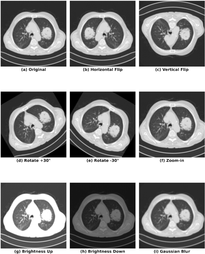
Figure 3: CT images after augmentation demonstrating rotation, zoom, and normalization to improve model generalization. Please click here to view a larger version of this figure.

These preprocessing techniques are required, and augmentation has been used across all the classes to ensure the model's robustness.

3. Model architecture

Adapting the novel Vision Transformer (ViT) framework to effectively handle complicated image data, the model architecture is intended to categorize CT scans into three categories: normal, benign, and malignant. With this method, 256 x 256 pixel input images are processed. To guarantee consistency and promote more efficient model learning, each image is put through several preprocessing operations, such as resizing and normalization. To improve the model's resilience to changes in image scale and orientation, the design begins with a data augmentation layer that uses methods including normalization, resizing, random rotations of 0.02 radians, and random zooms of up to 20%. After augmentation, the model takes 16 x 16 pixel patches out of every picture, thus every image has 256 patches.

Algorithm 1 defines the workflow the proposed model and how it is built and the fine tuning that is performed with respect to the model.

Algorithm 1: Lung cancer classification using Vision Transformers
Input: Set of CT images I from the IQ-OTH/NCCD dataset
Output: Classification results C into categories: Normal, Benign, Malignant
Preprocessing:
   for each image i in I do
i <- Resize(i, 256 x 256)         // Normalize and resize images
i <- Normalize(i)
i <- DataAugmentation(i)        // Apply random rotations and zooms
   end for
Model Setup:
  Initialize Vision Transformer (ViT) Model
  Set number of patches P = 16 x 16
  Set number of heads H = 6 in multi-head attention
Training:
  for epoch = 1 to MaxEpochs do
    for each batch b in I do
      Patches <- ExtractPatches(b, P)
      EncodedPatches <- PatchEncoder(Patches)
      AttentionWeights <- MultiHeadAttention(EncodedPatches, H)
      ClassLogits <- TransformerEncoder(AttentionWeights)
      Loss <- ComputeLoss(ClassLogits, TrueLabels)
      UpdateModelWeights(Loss)
    end for
    if EarlyStoppingCriteriaMet (Val_Loss No Improvement Patience = 5 Epochs) then
      break
    end if
  end for
 Validation:
  Split data into TrainingSet (80%) and ValidationSet (20%)
  ComputeValidationMetrics(ValidationSet)
Evaluation:
  C <- Classify(I)
  ComputePerformanceMetrics(C)
  Return C

To preserve the spatial relationships between patches, these patches are flattened (equation 1) into 768-dimensional vectors (because each patch has 16 x 16 x 3 = 768) and then sent through a patch encoding layer, which projects each vector into a 64-dimensional space by integrating positional embeddings. The core of the architecture comprises eight transformer layers, each featuring a multi-head attention mechanism with six heads, allowing the model to focus on different parts of the image simultaneously and capture a broad range of features. It is represented using equations 2, 3, and 4.

Where µ is the mean and σ² is the variance of the input x, and ϵ is a small constant to prevent division by zero.

Where Q is the query matrix, K is the key matrix, V is the value matrix, and d_k is the dimension of the key vectors.

Where W_i^Q, W_i^K, and W_i^V are the learned weight matrices for queries, keys, and values, respectively, and W^O is the output weight matrix.

The block diagram of the proposed model has been shown in Figure 4.

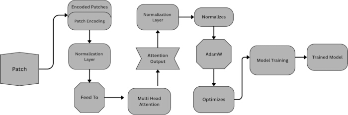
Figure 4: Block diagram of the Vision Transformer model with MLP head, detailing major processing layers and architecture. Please click here to view a larger version of this figure.

Each transformer layer includes a multi-layer perception (MLP) with hidden units first scaled up to 128 and then back down to 64, effectively expanding and compressing the information flow to capture complex dependencies.

Dropout is strategically applied at a rate of 0.1 within the attention mechanisms and MLPs to prevent overfitting. The output from the transformer encoder is processed through an MLP head consisting of two dense layers with 2,048 and 1,024 units, respectively, employing Gaussian Error Linear Units (GELU) for activation, which has been shown to perform well in deep learning applications. This is achieved using equation 5.

Where W₁ and W₂ are weight matrices, b₁ and b₂ are biases, and GELU is the activation function used.

A dropout of 0.1 was used in the transformer layers to prevent overfitting without losing important feature information. The GELU activation function was utilized for its smooth non-linear characteristics, which promote gradient flow and convergence in transformer-based models. The dropout is regularized using equation 6.

Where p is the dropout rate (e.g., 0.1 or 0.5), and the dropout layer randomly sets a fraction p of input units to zero during training.

A dropout rate of 0.5 in these layers further aids in mitigating overfitting. The final layer of the model is a logits layer (equation 7) that outputs three class logits corresponding to the categories of normal, benign, and malignant, using a sparse categorical cross entropy loss function (equation 8) appropriate for this multi-class classification setting.

Where z_i is the logits vector for class i, SoftMax(z_i)) represents the predicted probabilities, and y_i is the true class label.

The model is compiled with the AdamW optimizer (equations 9, 10, 11, 12, and 13), an extension of the Adam optimizer that more effectively handles weight decay, set at a learning rate of 0.001 and weight decay of 0.0001, optimizing both the learning speed and model stability.

Where m_t and v_t are the first and second moments of the gradients,  and  are the bias-corrected moments, η is the learning rate, and ϵ is a small constant to prevent division by zero.

The model, when trained, uses a batch size of 32 to take advantage of GPU acceleration for quicker calculation and is configured to train for 100 epochs.

But training has an early stopping mechanism on validation loss to limit training when the model stops improving to save computational resources and avoid overtraining of 5 consecutive epochs. Model performance is tracked with metrics like sparse categorical accuracy and top 2 accuracy, which inform about the model's classification ability across the most probable predicted categories. Callbacks for model training encompass checkpointing that will save the highest-performing model according to validation accuracy to ensure that the most successful version of the model is kept once the training process is over. This robust and well-planned architecture leverages the capabilities of transformers to process medical imaging data with a highly advanced approach to utilizing contemporary AI methods for major applications in healthcare diagnostics.

4.Training and validation

The model was trained in a Kaggle environment using an NVIDIA P100 GPU, and mini-batch gradient descent with a batch size of 32 was used during the training process. The optimizer used during training was AdamW with a learning rate of 0.001 and weight decay of 0.0001; this was a good balance between a fast convergence and some regularization. The model was trained for 100 epochs, however, early stopping on validation loss with a patience of 5 epochs was used. To put it simply, if the training did not improve validation loss for 5 continuous epochs, the training would stop for over fitting and computational efficiency. In most cases, this model restored weights from the epoch with the least validation loss, indicating it was performing optimally and did not need to run the entire 100 epochs. A total of about 32 minutes to train the model.

During training, metrics included sparse categorical accuracy and top-2 accuracy, monitored on both training and validation sets. These metrics provide insight into how often a model predicts the correct class and if the correct class is within the top two predictions, which in medical applications is of importance because high-confidence misclassifications may have significant consequences. The learning curves for loss and accuracy are visualized in Figure 5.

.

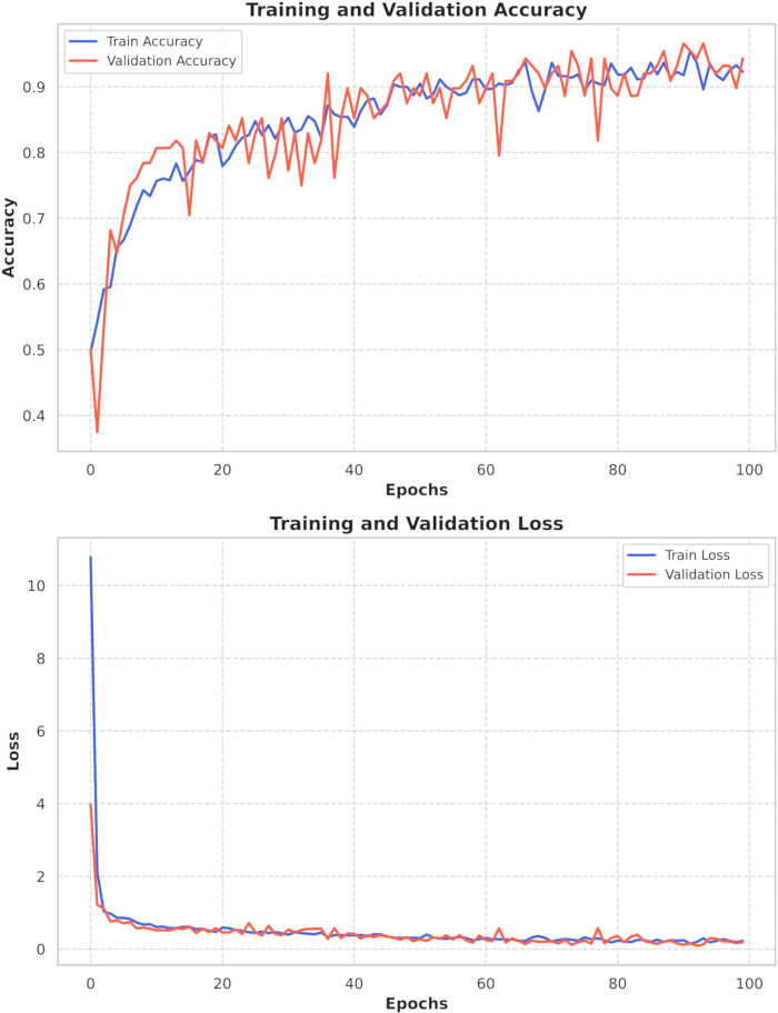
Figure 5: Training and validation accuracy and loss curves over 50 epochs showing stable learning and minimal overfitting. Please click here to view a larger version of this figure.

No cross-validation was performed in the present study. This setup allowed for efficient experimentation with model architecture, including adjustments to transformer layers and the sizes of MLP heads, while ensuring the model generalized well on unseen validation data.

5. Statistical analysis

The performance of the Vision Transformer model was statistically analyzed based on the IQ-OTH/NCCD lung cancer dataset. Precision, recall, F1-score, and accuracy were calculated using equations 14,15,16,17 respectively. These four are considered the conventional measures to use for classification tasks, in that they can reveal information about the performance of the model in classifying and classifying on a per-class basis for each class.

Recall is a measure of a model’s ability to identify all the relevant instances in a class, while precision is the proportion of positive identifications that were actually correct. The F1-score balances recall and precision when both are important.
The performance measures used for this assignment were the Matthews Correlation Coefficient (MCC)-equation 18- and Cohen's Kappa-equation 19.

Where P₀ is the observed agreement while P_e is the expected agreement.

The MCC is an all-encompassing measurement of classification performance, taking into account both true positives and negatives, false positives, and false negatives. Its value can be between -1 and 1, with 1 being perfect prediction, 0 being random prediction, and -1 being complete disagreement between the predicted and true labels. The MCC was of value for comparisons across different model performances when applied to imbalanced datasets and providing a measure that is balanced regardless of differing class sizes. 

As part of additional statistical analysis, the F2 score, prioritizing recall, was computed as shown by equation 20.

The model's performance was also quantified using Mean Squared Error (MSE), Root Mean Squared Error (RMSE), and Mean Absolute Error (MAE) - which are typically measurements for regression tasks but modified here for the classification task to quantify how large on average the error was without regard for direction.

In order to determine if it would be practical to integrate ViTs within consumer-focused healthcare devices, we carried out extensive performance evaluation results solely focusing on temporal efficiency of the model. We created functions to report the time taken to predict a single or simply multiple images, as this becomes particularly relevant for real-time applications. For each image, prior to starting to predict, data is first pre-processed to be in the shape of the input image desired by the model. The time the prediction started and the time the prediction completed we recorded to obtain the results of time and latency. Time and average latency was calculated using equation 21 and equation 22 respectively.

Where:

• N is the number of images (samples).
• tend is the time recorded after predicting the i-th image.
• tstart is the time recorded before predicting the i-th image.

Further experiments were performed to evaluate the robustness of the Vision Transformer model we proposed by systematically introducing additional noise and blur to the images. Gaussian noise was added to every pixel with a noise factor of 0.4 while clipping pixel values in the range of [0,1]. The blurring factor was diminished via Gaussian blur with a kernel size of 45× 45. These experiments are designed to evaluate the model comprehensively under simulated perceptive image quality degradations.

Results

The Vision Transformer model demonstrated exceptional results on a multiple evaluation metrics on the IQ-OTH/NCCD lung cancer datasets, effectively differentiating normal, benign, and malignant CT images. Overall model performance reached a high accuracy of 98.18% across the test dataset comprised of 220 images. This extremely high accuracy indicates that the model is able to generalize very effectively and can therefore be used in a clinical setting.

Discussion

It has achieved remarkable results in the evaluation and implementation of the Vision Transformer model on the IQ-OTH/NCCD lung cancer dataset with high accuracy. The general accuracy of classifying a CT scan as normal, benign, and malignant is 98.18% using this model.

This superior accuracy is further proven by the model's performance in the other key scores, such as 100% precision for malignant case detection, which is very important in early diagnosis and management.

Materials

List of materials used in this article

Name	Company	Catalog Number	Comments
A100 GPU (CUDA)	NVIDIA	CUDA Version 11.6	GPU acceleration for model training and evaluation.
AMD EPYC-7502P CPU	AMD	N/A	Processor used for high-performance computing.
Gigabit Ethernet	Intel	N/A	Networking for peer-to-peer secure communication in CPS.
Matplotlib	Python Software Foundation	Version 3.5	Visualization library for plotting results.
Paillier Cryptosystem	Open Source (implemented via TenSEAL)	N/A	Enables additive homomorphic encryption on gradients.
PySyft	OpenMined	Version 0.6.0	Differential privacy and federated learning library.
Python (Anaconda Distribution)	Anaconda Inc	Version 3.9	Includes pre-installed packages and environment management tools, Used for scripting and framework development.
PyTorch	Meta AI	Version 1.12	Deep learning framework for training models.
RAM	Corsair	256 GigaByte (GB)	High memory support for intensive training.
Scikit-learn	Python Software Foundation	Version 1.1	Machine learning tools for performance evaluation.
Seaborn	Python Software Foundation	Version 0.11	Statistical data visualization library.
SSD Storage	Seagate	1 TeraByte (TB)	For fast data storage and retrieval.
TenSEAL	OpenMined	Version 0.3	Homomorphic encryption library for secure aggregation.
TensorFlow	Google	Version 2.9	Deep learning framework for diffusion models.
Ubuntu OS	Canonical	Version 20.04 LTS	Operating system used for all experiments.

References

- Wang, L., et al. Transformer-based deep learning model for the diagnosis of suspected lung cancer in primary care based on electronic health record data. EBioMedicine. 110, 105442(2024).
- Kshatri, S. S., Singh, D. Convolutional neural network in medical image analysis: a review. Arch. Comput. Methods Eng. 30 (4), 2793-2810 (2023).
- Atabansi, C. C., et al. A survey of transformer applications for histopathological image analysis: new developments and future directions. Biomed. Eng. Online. 22 (1), 1-26 (2023).
- Xu, H., et al. Vision transformers for computational histopathology. IEEE Rev. Biomed. Eng. 17, 63-79 (2024).
- Xia, K., Wang, J. Recent advances of transformers in medical image analysis: a comprehensive review. MedComm Future Med. 2 (1), e38(2023).
- Kim, J. W., et al. Systematic review of hybrid vision transformer architectures for radiological image analysis. J. Imaging Inform. Med. , (2025).
- Suresh, S., Mohan, S. ROI-based feature learning for efficient true positive prediction using convolutional neural network for lung cancer diagnosis. Neural Comput. Appl. 32 (20), 15989-16009 (2020).
- Fanizzi, A., et al. Comparison between vision transformers and convolutional neural networks to predict non-small lung cancer recurrence. Sci. Rep. 13 (1), 48004(2023).
- Alijani, S., et al. Vision transformers in domain adaptation and domain generalization: a study of robustness. Neural Comput. Appl. 36 (29), 17979-18007 (2024).
- Rane, N. Transformers for medical image analysis: applications, challenges, and future scope. SSRN Electron. J. , (2023).
- Taye, M. M. Theoretical understanding of convolutional neural network: concepts, architectures, applications, future directions. Computation. 11 (3), 52(2023).
- Mothkur, R., Veerappa, B. N. Classification of lung cancer using lightweight deep neural networks. Procedia Comput. Sci. 218, 1869-1877 (2023).
- Alsadoon, A., et al. DFCV: a framework for evaluation deep learning in early detection and classification of lung cancer. Multimed. Tools Appl. , (2023).
- Mohamed, T. I. A., et al. Automatic detection and classification of lung cancer CT scans based on deep learning and ebola optimization search algorithm. PLoS ONE. 18 (8), e0285796(2023).
- Sangeetha, S. K. B., et al. An enhanced multimodal fusion deep learning neural network for lung cancer classification. Syst. Soft Comput. 6, 200068(2024).
- Raza, R., et al. Lung-EffNet: lung cancer classification using EfficientNet from CT-scan images. Eng. Appl. Artif. Intell. 126, 106902(2023).
- Dunn, B., et al. Automated classification of lung cancer subtypes using deep learning and CT-scan based radiomic analysis. Bioengineering. 10 (6), 690(2023).
- Wani, N. A., et al. DeepXplainer: an interpretable deep learning based approach for lung cancer detection using explainable artificial intelligence. Comput. Methods Programs Biomed. 243, 107879(2024).
- Subash, J., Kalaivani, S. Dual-stage classification for lung cancer detection and staging using hybrid deep learning techniques. Neural Comput. Appl. 36 (14), 8141-8161 (2024).
- Yin, P., et al. Imaging of tumor boundary based on multielements and molecular fragments heterogeneity in lung cancer. IEEE Trans. Instrum. Meas. 70, 1-7 (2021).
- AL-Huseiny, M. S., Sajit, A. S. Transfer learning with GoogLeNet for detection of lung cancer. Indones. J. Electr. Eng. Comput. Sci. 22 (2), 1078-1086 (2021).
- Gupta, A., et al. UDCT: lung cancer detection and classification using U-net and DARTS for medical CT images. Multimed. Tools Appl. 84 (18), 19065-19085 (2024).
- Bagheri Tofighi, A., et al. Improving lung cancer detection via MobileNetV2 and stacked-GRU with explainable AI. Int. J. Inf. Technol. 17 (2), 1189-1196 (2024).
- Kareem, H. F., et al. Evaluation of SVM performance in the detection of lung cancer in marked CT scan dataset. Indones. J. Electr. Eng. Comput. Sci. 21 (3), 1731-1738 (2021).
- Lung tumor detection and recognition using deep convolutional neural networks. Solyman, S., Schwenker, F. Pan-Afr. Conf. Artif. Intell, , 79-91 (2023).
- Das, S., et al. Automated prediction of lung cancer using deep learning algorithms. Applied Artificial Intelligence. , 93-120 (2023).
- Abe, A. A., et al. A robust deep learning algorithm for lung cancer detection from computed tomography images. SSRN Electron. J. , (2023).
- Mathews, A. B., Karani, K. P. Lung cancer segmentation and classification using integration of convolutional neural network & U-net network over CT images: a deep learning approach. Int. J. Manag. Technol. Soc. Sci. , 520-534 (2022).
- MAT-VIT: a vision transformer with MAE-based self-supervised auxiliary task for medical image classification. Han, Y., et al. 27th Int. Conf. Comput. Support Coop. Work Des. (CSCWD), , 2046-2052 (2024).
- Ko, J., et al. Optimization of vision transformer-based detection of lung diseases from chest X-ray images. BMC Med. Inform. Decis. Mak. 24 (1), 1-15 (2024).
- Apostolidis, K. D., Papakostas, G. A. A survey on adversarial deep learning robustness in medical image analysis. Electronics. 10 (17), 2132(2021).
- Hybrid design of CNN and vision transformer: a review. Long, H. 7th Int. Conf. Comput. Inf. Sci. Artif. Intell, , 121-127 (2024).
- Papanastasiou, G., et al. Is attention all you need in medical image analysis? A review. IEEE J. Biomed. Health Inform. 28 (3), 1398-1411 (2024).
- Advancing healthcare in low-resource environments through an optimization and deployment framework for medical multimodal large language models. El Mir, A., et al. 2024 IEEE EMBS Int. Conf. Biomed. Health Inform. (BHI), , 1-8 (2024).
Access restricted. Please log in or start a trial to view this content.