Biolayer Interferometry for Investigating Membrane Protein-Inhibitor Binding: TACAN Mutant and GsMTx4 As a Model System

Summary

This manuscript provides a detailed protocol for optimizing and conducting Bio-Layer Interferometry (BLI) experiments to study membrane protein-ligand interactions for detergent-solubilized membrane proteins. Using the interaction between the TMEM120A M207A mutant and the peptide inhibitor GsMTx4 as a model, this workflow outlines protein preparation, biosensor loading, and kinetic data acquisition.

Abstract

Bio-Layer Interferometry (BLI) is an efficient biophysical technique that enables real-time, quantitative analysis of biomolecular interactions. Although commonly used for soluble proteins, their application to membrane proteins remains challenging due to hydrophobicity and detergent dependence. This study presents an optimized BLI protocol for characterizing interactions between detergent-solubilized membrane protein and peptide inhibitor.

As a model system, the gating-modifier peptide Grammostola mechanotoxin 4 (GsMTx4) was tested against the multifunctional membrane protein mutant TMEM120A M207A. The FLAG-tagged TMEM120A variant was immobilized on anti-FLAG biosensors-representing a tag-based but fluorescent- and enzyme-label-free setup-and exposed to serial dilutions of GsMTx4 to measure association and dissociation rates.

The protocol integrates detergent optimization using Lauryl Maltose Neopentyl Glycol (LMNG) and complementary characterization by mass photometry and differential scanning fluorimetry (DSF). This workflow enables reliable kinetic measurements and is compatible with medium-throughput screening. The approach may be applicable to other membrane protein-ligand systems where detergent stability is maintained. Overall, the study highlights key parameters influencing immobilization efficiency and analyte delivery, supporting the potential utility of BLI in inhibitor profiling and mechanistic studies of membrane protein interactions.

Introduction

Membrane proteins play central roles in essential physiological processes, including signal transduction, ion and metabolite transport, and membrane organization. Given their involvement in cellular communication and homeostasis, they represent a substantial proportion of drug targets in clinical development. Understanding membrane protein-ligand interactions is critical for elucidating function and guiding therapeutic design. However, the amphipathic nature of these proteins and their dependence on lipid environments present significant challenges for purification, stabilization, and biophysical characterization.

Surface plasmon resonance (SPR) and isothermal titration calorimetry (ITC) are widely used techniques for studying the kinetics and thermodynamics of membrane protein-ligand interactions^1,2. When appropriately optimized, both methods can provide detailed quantitative insights, even for detergent-solubilized or reconstituted membrane proteins. Microscale thermophoresis (MST) has also been successfully applied to assess binding affinities under near-native conditions, particularly for membrane proteins³. Nevertheless, these approaches can be limited by substantial sample consumption, difficulties in maintaining membrane protein stability, or restricted compatibility with certain detergent systems.

Bio-Layer Interferometry (BLI) is a real-time optical technique that enables quantitative measurement of biomolecular interactions, including those involving detergent- or amphipol-solubilized membrane proteins. Along with the previously mentioned biophysical techniques, BLI offers an efficient platform that enables the direct measurement of binding kinetics, including association (k_on), dissociation (k_off), and equilibrium dissociation constants (K_D), with lower sample concentrations and straightforward adaptation to detergent- or Nanodisc-solubilized membrane proteins. It is also noteworthy that, like all biophysical technologies, BLI has its own limitations, which will be mentioned in the Discussion section.

BLI detects shifts in the interference pattern of white light reflected from a biosensor tip, with changes in optical thickness corresponding to biomolecular binding events. These shifts (Δλ, in nm) are recorded as sensorgrams and are proportional to the mass bound at the sensor surface. BLI has been widely applied to protein-protein and protein-ligand interactions (including peptides and small molecules) and is suitable for affinity ranges from nanomolar to micromolar⁴. Its flexibility, low sample consumption, and relatively simple setup make it a potentially advantageous tool for studying detergent-solubilized membrane proteins^5,6,7.

This study presents a BLI protocol for characterizing the interaction between TMEM120A M207A, a membrane protein, and Grammostola mechanotoxin 4 (GsMTx4), a peptide inhibitor. TMEM120A has been proposed as a mechanosensitive ion channel involved in mechanical pain detection⁸; however, its ion channel activity remains controversial. Multiple studies have reported the absence of mechanosensitive currents when TMEM120A is expressed in heterologous systems such as HEK293 or CHO cells^1,9,10,11. To date, more than four cryo-EM studies have resolved the structure of TMEM120A in the closed state, and no open conformation has been observed^1,9,10,11.

Molecular dynamics simulations and electrophysiological analyses indicate that methionine 207 (M207) in wild-type human TMEM120A may act as a gating barrier within the ion conduction pathway¹¹. Mutation of this residue to alanine (M207A) has been shown to increase ion permeability, likely by altering helix packing and displacing hydrophobic side chains such as Phe223. Consequently, the M207A mutant was selected for binding studies with GsMTx4.

GsMTx4 is a gating-modifier peptide derived from spider venom that inhibits mechanosensitive cation channels. It consists of a 32 amino acid sequence and has a molecular weight of 4 to 5 kDa, including Piezo and TRP channels, primarily by interacting with the lipid bilayer rather than directly blocking the pore^12,13. Previous studies have demonstrated that GsMTx4 reduces TMEM120A activity in artificial bilayer systems⁸. In the BLI assays, the TMEM120A M207A mutant was immobilized on anti-FLAG biosensors and exposed to increasing concentrations of GsMTx4, allowing measurement of association (k_on) and dissociation (k_off) rates.

This work provides a detailed protocol for detergent optimization and kinetic analysis using Bio-Layer Interferometry (BLI). While BLI has some limitations, such as potential artifacts from sensor overloading or mass transport effects and reduced suitability for fast association rate (k_on) interactions, it is a useful method for studying membrane protein-ligand interactions under controlled detergent-solubilized conditions. The protocol is suitable for systems with moderate-to-low binding affinities (typically in the nanomolar to micromolar range) and can be adapted to other hydrophobic targets when appropriate controls and buffer conditions are applied.

Protocol

1. Protein purification and sample optimization

1. Cell culture and transfection
   1. Grow HEK293T/SF17 suspension cells in serum-free medium supplemented with 20 mM L-glutamine in a shaking incubator set at 120 RPM, 37 °C, 80% humidity, and 8% CO₂. Maintain cells by passaging up to passage five; allow cells to reach a density of approximately 5 × 10⁶ cells/mL.
   2. Transfect the cells with the TMEM120A M207A plasmid (N-terminal FLAG-Linker-3C-Linker-TMEM120A M207A) in the pCDNA3.1 vector using a commercial transfection reagent according to the manufacturer's instructions (see the Table of Materials).
   3. Pellet transfected cells by centrifugation at 5,000 × g for 15 min at 4 °C. Store the cell pellet at -80 °C until purification.
2. Cell lysis and solubilization (Figure 1)
   1. Resuspend a 30 mL cell pellet in solubilization buffer containing 100 mM 4-(2-hydroxyethyl)-1-piperazineethanesulfonic acid (HEPES), pH 7.8; 300 mM NaCl; 0.5% (w/v) or 4.98 mM lauryl maltose neopentyl glycol (LMNG); 1x protease inhibitor cocktail; 50 µg of DNase I; 10% (v/v) Glycerol.
   2. Lyse the cells by ultrasonication at 25% amplitude using a 20 s on/20 s off pulse cycle for 15 min, while keeping the sample on ice to prevent overheating.
   3. Clarify the lysate by centrifugation at 25,800 × g for 45 min at 4 °C.
3. Affinity purification using anti-FLAG resin
   1. Equilibrate anti-FLAG M2 resin with equilibration buffer containing 25 mM HEPES, pH 7.8; 200 mM NaCl; 0.05% (w/v) or 0.4975 mM LMNG; 10% (v/v) Glycerol.
   2. Incubate the clarified supernatant with equilibrated resin for 2 h at 4 °C on a rocker.
   3. Wash the resin 2x with wash buffer containing 25 mM HEPES, pH 7.8; 150 mM NaCl; 0.05% (w/v) or 0.4975 mM LMNG; 10% (v/v) Glycerol.
   4. Elute the bound protein using elution buffer containing 25 mM HEPES, pH 7.8; 400 mM NaCl; 0.001% (w/v) or 0.00995 mM LMNG; 10% (v/v) Glycerol; 200 µg/mL FLAG peptide.
4. Concentration and size-exclusion chromatography (SEC)
   1. Concentrate the eluted protein to ~500 µL using a centrifugal filter unit with a 30 kDa cutoff.
   2. Perform SEC using the referenced size exclusion column equilibrated with 25 mM HEPES, pH 7.8; 200 mM NaCl; 0.00015% (w/v) or 0.00149 mM LMNG.
   3. Collect and pool peak fractions corresponding to the target protein.
   4. Concentrate pooled fractions to ~3 mg/mL final concentration. After affinity purification, confirm that the TMEM120A M207A protein monomer appears at approximately 43 kDa on SDS-PAGE (Figure 2A). For SEC, confirm that the purified protein in LMNG elutes as a monodisperse peak corresponding to approximately 150 kDa, which represents the TMEM120A M207A dimer together with the LMNG detergent micelle (Figure 2B).
      NOTE: Occasionally, the monomer protein band may appear around 50 kDa, which is common for detergent-solubilized membrane proteins, as boiling membrane protein samples is not typical.

2. Thermal stability analysis by nano differential scanning fluorimetry (NanoDSF)

1. Dilute the purified TMEM120A M207A protein to 0.15 mg/mL in SEC buffer (25 mM HEPES, pH 7.8, 200 mM NaCl, 0.00015% LMNG).
2. Load 10 µL of each sample into high-sensitivity capillaries.
3. Run the thermal shift assay on a NanoDSF instrument with a temperature ramp from 25 °C to 90 °C.
4. Use compatible software to set up the assay and perform automated analysis.
5. Confirm that a single thermal transition (T_m) curve is visible, indicating a cooperative unfolding event (Figure 3).

3. Mass photometry for oligomeric state determination

1. Prepare a sample diluted to 80 nM in SEC buffer (25 mM HEPES, pH 7.8, 200 mM NaCl, 0.00015% LMNG).
2. Place the sample in precleaned mass photometry-compatible slides.
3. Acquire data using standard settings and calibrate using protein standards.
4. Process data with analysis software to generate mass distribution histograms (Figure 4A-C).

4. Biolayer interferometry (BLI) protocol

NOTE: This protocol describes a BLI kinetic assay designed to study interactions between FLAG-tagged TMEM120A M207A and ligands such as GsMTx4, using a 384-well microplate format. Although developed for TMEM120A, the workflow can be adapted for other membrane proteins. All experiments were conducted using an optical interferometry platform with FLAG biosensor probes to immobilize FLAG-tagged TMEM120A M207A. A 384-well black microplate was used with an optimized size-exclusion chromatography (SEC) buffer containing 25 mM HEPES, 200 mM NaCl, 0.00015% (w/v) LMNG, and 0.0005% Tween-20, pH 7.8. Tween-20 was included to minimize nonspecific binding. Protein concentration was maintained at 250 nM, and all assays were performed in duplicate to ensure reproducibility.

1. Assay design considerations
   1. Temperature equilibration
      1. Prior to starting the BLI assay, equilibrate all assay components-including buffers, samples, and biosensor probes-to room temperature (approximately 20-25 °C). During data acquisition, maintain the assay temperature at 30 °C, which is recommended for kinetic analyses to optimize protein stability, ligand binding, and reproducibility.
         NOTE: This equilibration step ensures consistent kinetic profiles and minimizes artifacts caused by temperature fluctuations during the experiment. Allow sufficient time (at least 10-15 min) for all reagents and biosensors to reach thermal equilibrium before beginning the assay.
   2. Sensor hydration and regeneration
      1. Hydrate new FLAG biosensors in 250 µL of BLI-compatible buffer (SEC buffer containing 25 mM HEPES, 200 mM NaCl, 0.00015% w/v LMNG, and 0.0005% Tween-20, pH 7.8) in the Max plate for a minimum of 10 min prior to use.
         NOTE: Handle biosensors carefully with clean, dust-free tweezers to avoid contamination, which can interfere with signal acquisition and lead to inconsistent results. For sensor reuse, perform regeneration using Q buffer (0.3 M glycine, pH 3.8). Proper hydration and regeneration are critical to maintain sensor performance and reproducibility, especially when working with detergent-solubilized membrane proteins, which are sensitive to environmental conditions.
   3. Buffer handling
      1. Avoid air bubbles when dispensing liquids, as they can interfere with optical signal acquisition.
   4. Buffer composition and consistency
      1. Use a buffer that minimizes nonspecific interactions while preserving protein function. For TMEM120A M207A, prepare the buffer containing 25 mM HEPES, 200 mM NaCl, 0.00015% (w/v) LMNG, 0.0005% (w/v) Tween 20, pH 7.8.
   5. Protein immobilization
      1. Optimize ligand loading to achieve 50-80% sensor saturation. Use a fixed concentration of protein at 250 nM, with a typical loading duration of approximately 120 s. Load FLAG-tagged TMEM120A M207A (250 nM) onto the biosensor for 120 s to achieve 50-80% saturation.
      2. Confirm that the biosensor signal reaches 50 - 80% of the maximum binding capacity during the loading phase.
         NOTE: Signals below 50% may indicate insufficient protein immobilization, whereas signals above 80% can introduce mass transport limitations or steric hindrance, potentially compromising kinetic measurements.
      3. To assess potential mass transport effects, perform a control experiment in which the analyte concentration (e.g., 100 nM GsMTx4) is held constant while varying the loading levels of TMEM120A-M207A on FLAG biosensors (Supplemental Figure S1).
         NOTE: Subsequent kinetic measurements-including association, dissociation, global binding fits, and determination of k_on and k_off-were not significantly different from those obtained in the main assay. This result indicates that TMEM120A loading within the 50-80% range does not introduce significant mass transport artifacts, confirming that the biosensor loading level is appropriate for reliable kinetic analysis.
   6. K_D estimation
      1. Determine the binding affinity (K_D) by testing analyte (GsMTx4) concentrations of 0 µM, 5 µM, 10 µM, 20 µM, 30 µM, 50 µM, and 100 µM.
   7. Background signal controls
      1. Include appropriate controls to accurately subtract background signals and ensure reliable kinetic measurements.
      2. Use a reference FLAG probe to account for nonspecific binding or drift that may occur during the assay.
         NOTE: This reference probe should not have the target protein immobilized and serves as a baseline to correct the signal obtained from the sample-containing probes.
      3. Subtract the Reference signal from the sample signal to analyze only specific interactions between FLAG-tagged TMEM120A M207A and analytes.
         NOTE: Verify that the reference FLAG probe shows minimal signal throughout the assay. A stable, low baseline indicates negligible nonspecific binding. If the reference signal fluctuates or increases, reassess buffer composition, probe handling, or sample preparation to reduce nonspecific interactions before proceeding with kinetic analysis.
2. Configuration of basic assay parameters for kinetics analysis
   1. Set the data acquisition frequency to 5 Hz to collect 5 data points/s (recommended for all kinetics assays).
   2. Select 384-well plate as the plate format.
   3. Set the shaker speed to 1,000 RPM and the temperature between ambient and 30 °C (30 °C used in this experiment for optimal kinetics results).
3. Configure the plate setup.
   1. Navigate to the Plate Setup Tab and define well assignments for both the 384-well plate and Max plate.
   2. Assign well functions on the 384-well plate.
      NOTE: The symbols and annotations used for both the 384-well plate and the Max Plate are summarized in Supplemental Table S1.
      1. Label wells according to the role: buffer, protein (loading), ligand (sample).
      2. Annotate protein loading wells with concentration (e.g., 250 nM) for kinetic assays.
         ​NOTE: Accurate labeling is essential for calculating k_on and K_D (see Supplemental Figure S2A).
   3. Configure the Max plate map (probe plate).
      1. Assign biosensor probes to appropriate wells.
      2. If probe regeneration is planned, assign wells for regeneration and neutralization buffers. Clearly label these wells in the software to ensure proper automation during regeneration (see Supplemental Table S2).
         NOTE: The assay buffer consisted of 25 mM HEPES (pH 7.8), 200 mM NaCl, 0.00015% (w/v) LMNG, and 0.0005% (v/v) Tween-20. The regeneration step of the anti-FLAG biosensor probes was performed using Q buffer containing 0.3% glycine (pH 3.8), followed by a neutralization step with the assay buffer (25 mM HEPES, 200 mM NaCl, 0.00015% LMNG, and 0.0005% Tween-20, pH 7.8).
4. Select the Assay Steps tab.
   1. Navigate to the Assay Steps tab to configure the kinetic assay workflow. Specify well positions for each assay phase, including baseline, protein loading, association, and dissociation (see Supplemental Figure S3).
   2. Select the appropriate step type from the dropdown menu. Ensure that the association and dissociation steps are correctly labeled for accurate kinetic analysis.
   3. Enter the duration for each step in seconds to define exposure times for all interaction phases.
      1. Set the baseline step duration to allow sensor equilibration before protein loading (60 s).
      2. Set the protein loading step duration to achieve desired ligand immobilization levels of (60 s) (Figure 5).
      3. Set the association step duration to allow sufficient analyte binding (300 s) (Figure 5).
      4. Set the dissociation step duration to adequately capture analyte unbinding kinetics (600 s) (Figure 5).
   4. Set the shaker speed (RPM) for each step to maintain consistent mixing and optimal data quality (1,000 RPM).
5. Align and filter step (see Supplemental Figure S4 and Supplemental Figure S5)
   1. Perform raw data correction by adjusting the data range as needed to remove artifacts from kinetic steps.
   2. To align the Y-axis, align the data at the start of the association step by selecting Association under Align Step Type and activating the Begin option.
   3. Enable the Interstep correction option to maintain continuity between steps during standard kinetic assays.
   4. Filtering: Apply data smoothing to reduce signal noise without distorting trends. Select Processed to compare smoothed data with raw signals.
6. Set a reference step (see Supplemental Figure S6).
   1. Designate a reference probe by selecting the reference probe and click the Ref. Probe button.
   2. Select sample probes by clicking on the corresponding column numbers for the sample probes.
   3. To define the subtraction function, open the Formula Editor, click Edit Formula, and define the subtraction function to remove the background.
   4. Review Table view to confirm that reference subtraction has been applied correctly.
7. Binding fitting step
   1. Navigate to the Fitting tab and define analysis parameters (Supplemental Figure S7).
   2. Data selection: Include both association and dissociation phases for local kinetic fitting. Exclude outliers manually if they display poor curve fitting or erratic signal.
   3. Binding model selection: Choose the 1:1 binding model to fit the data unless complex behavior is observed. Review curve overlays and residuals to validate model suitability.
   4. Fitting strategy: Select one of the following fitting strategies depending on data quality and experimental objectives:
      1. Local: Fits each analyte concentration individually, allowing independent evaluation of association and dissociation kinetics.
      2. Global: Fits all analyte concentrations simultaneously using a single set of kinetic parameters, providing an overall model for the dataset.
      3. Full: Fits both association and dissociation phases globally across all concentrations.
      4. Partial: Fits only the association phase, ignoring dissociation.
         NOTE: BLI data were analyzed using a 1:1 Langmuir binding model with local, full fitting. Local fitting ensures that each analyte concentration is treated independently, providing an accurate representation of association kinetics while minimizing artifacts from heterogeneity in the dissociation phase. This approach avoids overfitting in regions with variable or unstable signals, allowing more reliable estimation of kinetic parameters (k_on and k_off) (Table 1 and Table 2).
8. Kinetic analysis
   1. Review of fitted curves and residuals: Examine the fitted curves and corresponding residuals to assess the quality and validity of the model. Confirm that residuals are randomly distributed around zero without systematic deviations (see Figure 4E for representative residuals).
   2. Exclusion of poorly fitting data: Remove analyte concentrations that exhibit flat, noisy, or otherwise unreliable signals to improve the overall model accuracy.
      NOTE: For example, the 10 µM concentration was excluded from fitting due to overlapping with the 5 µM dataset, which could distort kinetic parameter estimation (see Figure 6A,B).

Results

The TMEM120 M207A mutant was expressed in HEK293SF-17 suspension cells using a pCDNA3.1 vector encoding an N-terminal FLAG tag Figure 1. Transient transfection enabled recombinant protein expression. After cell harvest, membrane proteins were solubilized in 0.5% lauryl maltose neopentyl glycol (LMNG), a non-ionic detergent suitable for maintaining membrane protein solubility.

The solubilized fraction was subjected to affinity purification using anti-FLAG M2 resin. The resin was washed with buffer containing 0.01% LMNG to remove non-specifically bound proteins, and TMEM120 M207A was eluted in buffer containing 0.001% LMNG. The elution was concentrated using centrifugal filters with molecular weight cutoffs of either 30 kDa or 100 kDa, depending on sample yield. Further purification was performed by size-exclusion chromatography (SEC). The final SEC step was carried out in a buffer containing 0.00015% LMNG, producing a monodisperse elution profile consistent with a homogeneous and stable protein preparation suitable for subsequent structural and functional analyses (Figure 2B).

Optimization and biophysical characterization of FLAG-tagged TMEM120 M207A are summarized in Figure 2. Expression and purification were confirmed by SDS-PAGE, which showed a single band at approximately 50 kDa. The observed migration was slightly above the expected molecular weight of the monomeric form (Figure 2A), likely due to the nonboiled sample prior to electrophoresis. The SEC chromatogram displayed a single, symmetric peak eluting at a volume corresponding to an apparent molecular mass of approximately 150 kDa in 0.00015% (w/v) LMNG (Figure 2B), consistent with the TMEM120A M207A dimer in LMNG detergent micelles. This elution behavior exhibits a homogeneous and monodisperse protein population, making it suitable for downstream biophysical characterization.

The detergent micelle properties of LMNG under the experimental buffer conditions were analyzed using mass photometry. Measurements were performed in SEC buffer having varying concentrations of LMNG in the absence of protein to evaluate the contribution of detergent micelles to the clear molecular mass. At 0.001% (w/v) LMNG, a concentration above the critical micelle concentration (CMC), the predominant peak was detected at approximately 69 kDa, corresponding to LMNG micelles alone without any associated protein (Figure 4A). When the LMNG concentration was reduced to 0.0001% (w/v), below the CMC, the major species shifted to ~48 kDa, indicating the presence of smaller residual LMNG aggregates or submicellar assemblies without protein (Figure 4B). Further in (Figure 4C), TMEM120A M207A was diluted in SEC buffer containing different concentrations of LMNG to assess its oligomeric state by mass photometry. At 0.00001% LMNG (~20x below the CMC, magenta), a predominant peak was observed at approximately 42 kDa, corresponding to the monomer of TMEM120A M207A. At 0.00015% LMNG (~10x below the CMC, blue), the main population at ~86 kDa indicated the presence of dimers. Increasing the LMNG concentration to 0.001% (~2x above the CMC, orange) resulted in a major species ~150 kDa, consistent with protein-detergent complexes. At 0.002% LMNG (~4x above the CMC, green), a broad distribution centered near 180 kDa was detected, representing larger micelle-associated assemblies or higher-order oligomers. These results demonstrate that the LMNG concentration within the SEC buffer strongly influences the clear oligomeric state of TMEM120A M207A, with monomer-dimer equilibrium observed below the CMC and detergent-protein complex formation predominating above the CMC.

The thermodynamic stability of TMEM120A M207A collected from the main SEC peak and kept in SEC buffer (25 mM HEPES, 200 mM NaCl, 0.00015% (w/v) LMNG, pH 7.8) was evaluated by thermal denaturation analysis. The protein exhibited an inflection point at approximately 46 °C, corresponding to its melting temperature (T_m) under these detergent-solubilized conditions. This T_m value indicates moderate thermal stability, suggesting that TMEM120A M207A retains a properly folded conformation within LMNG micelles but may begin to unfold or aggregate at higher temperatures.

Biolayer interferometry (BLI) shows µM binding affinity of TMEM120A M207A to GsMTx4T. The traces in Figure 5 illustrate five experimental steps: (1) baseline, (2) TMEM120A M207A sample loading, (3) baseline to remove nonspecific binding and excess TMEM120A M207A, (4) association, and (5) dissociation. Wavelength shift (nm) is plotted over time for increasing concentrations of GsMTx4 (0, 5, 10, 20, 30, 50, and 100 µM) interacting with immobilized TMEM120A M207A.

During the initial baseline (step 1), the signal remained stable, confirming sensor equilibration in the buffer. TMEM120A M207A loading (step 2) produced a characteristic increase in signal, corresponding to ~50-80% probe saturation across sensors. The loading phase showed a slightly curved response rather than a sharp plateau, possibly reflecting partial mass transport limitation, where TMEM120A M207A diffusion to the sensor surface is slower than the binding rate -- an effect common for membrane or detergent-solubilized proteins that can influence apparent surface coverage.

The subsequent baseline step (step 3) effectively removed unbound or loosely attached TMEM120A M207A. During the association phase (step 4), increasing GsMTx4 concentrations resulted in clear, concentration-dependent increases in wavelength shift. During dissociation (step 5), the biosensor was placed in SEC buffer containing LMNG at ~10x below the CMC. The first 5-10 s of dissociation showed a rapid signal decrease, likely representing fast release of GsMTx4 from readily accessible sites, followed by a slower decay that may reflect more stable TMEM120A M207A-GsMTx4 complexes with slow dissociation kinetics. Reference probe signals remained flat throughout the experiment, indicating minimal nonspecific binding. Overall, these data demonstrate specific TMEM120A M207A-GsMTx4 interactions; however, the observed kinetics should be interpreted cautiously due to the detergent environment and potential mass transport effects.

The association and dissociation sensorgrams of the processed data after reference probe subtraction (Figure 6A) showed concentration-dependent responses for GsMTx4 in the range of 5-100 µM. Increasing ligand concentrations produced progressively higher wavelength shifts, followed by a gradual, slow decrease during the 200 s dissociation phase. The 10 µM dataset was excluded from fitting due to overlap with the 5 µM trace, which improved the overall model quality.

Kinetic analysis was performed using a 1:1 Langmuir association-dissociation model with a local full-fitting strategy, in which individual analyte concentrations were fitted independently within a shared kinetic framework (Figure 6B). The fitted curves (red) were in good agreement with the experimental traces, yielding an estimated dissociation constant (K_D) in the low micromolar range. Residual analysis (Figure 6C) did not reveal major systematic deviations, indicating that the applied model was appropriate for the dataset. Minor differences observed during the early association phase may reflect limitations in mass transport or the effects of the detergent micelle environment. Additional examples of fitted association and dissociation curves, residual plots, and fitting statistics across multiple assay replicates and probe positions are shown in Supplemental Figure S8.

In the raw data (Figure 5), the first 5-10 s of dissociation showed a rapid signal decrease, likely representing the fast release of GsMTx4 from readily accessible sites, followed by a slower decay that may reflect more stable TMEM120A M207A-GsMTx4 complexes with slow dissociation kinetics. Therefore, in Table 2, the first 100 s of dissociation were removed from fitting. The lack of systematic deviation indicates a good fit of the local full-fitting Langmuir 1:1 model for TMEM120A M207A at all tested concentrations (Figure 7).

Kinetic analysis of GsMTx4 binding to TMEM120A M207A revealed concentration-dependent association and dissociation behaviors across the 5-100 µM ligand range (Table 1). The observed association rate constants (k_on) increased modestly with rising GsMTx4 concentration, ranging from approximately 1.0 × 10⁻⁶ to 3.2 × 10^-6 1/M·s, while the estimated dissociation rate constants (k_off) remained near zero within the experimental error, suggesting a slow or negligible dissociation phase under the tested conditions. The calculated equilibrium dissociation constants (K_d) were in the low to mid-micromolar range (~0.8-3.3 µM), consistent with a moderate affinity interaction. Local Full fitting using a Langmuir 1:1 binding model yielded high-quality fits across all GsMTx4 concentrations, with correlation coefficients exceeding 0.99 and low relative χ² values for both association and dissociation phases (Table 1). The calculated equilibrium dissociation constants were consistent across concentrations and replicates, with K_D values in the low micromolar range (~1-2 µM), indicating moderate but specific binding between TMEM120A M207A and GsMTx4.

Replicate datasets at each concentration showed reproducibility, as indicated by high correlation coefficients (R² > 0.99) for both association and dissociation fits. The full and relative χ² values were low and comparable across replicates, further supporting the robustness of the 1:1 Langmuir binding model applied in the analysis. At higher ligand concentrations (≥50 µM), slightly increased k_on and K_D values were observed, which may reflect minor mass transport effects or local surface heterogeneity rather than true affinity changes. Kinetic consistency across multiple replicates and probe positions is further illustrated in Supplemental Figure S9.

The kinetic profiles demonstrate that GsMTx4 interacts specifically and stably with TMEM120A M207A, forming relatively stable complexes characterized by slow dissociation and micromolar binding affinity.

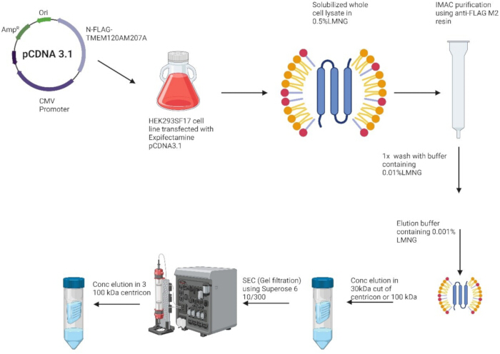
Figure 1: Purification workflow of TMEM120A M207A mutant expressed in HEK293SF-17 suspension cells. Schematic overview of the protein purification procedure. TMEM120A M207A was expressed from pCDNA3.1 plasmids in HEK293SF-17 cells. Cells were solubilized in 0.5% LMNG, followed by affinity purification using anti-FLAG M2 resin. The resin was washed with buffer containing 0.01% LMNG to remove non-specifically bound proteins. TMEM120A M207A was eluted in buffer containing 0.001% LMNG. The eluate was concentrated using either 100 kDa or 30 kDa molecular weight cutoff filters and further purified by size-exclusion chromatography in a buffer containing 0.00015% LMNG. Please click here to view a larger version of this figure.

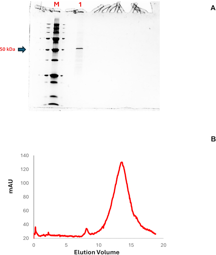
Figure 2: Size exclusion chromatography and SDS PAGE of purified TMEM120A M207A In LMNG detergent (A) SDS-PAGE of FLAG-tagged TMEM120A M207A purified by size-exclusion chromatography. The protein band appears at ~50 kDa in lane 1, corresponding to the expected monomer. (B) SEC profile of purified TMEM120A M207A on an SEC column in SEC buffer (25 mM HEPES, 200 mM NaCl, 0.00015% LMNG, pH 7.8). Protein elution indicates a predominant monodisperse species suitable for downstream biophysical assays. Please click here to view a larger version of this figure.

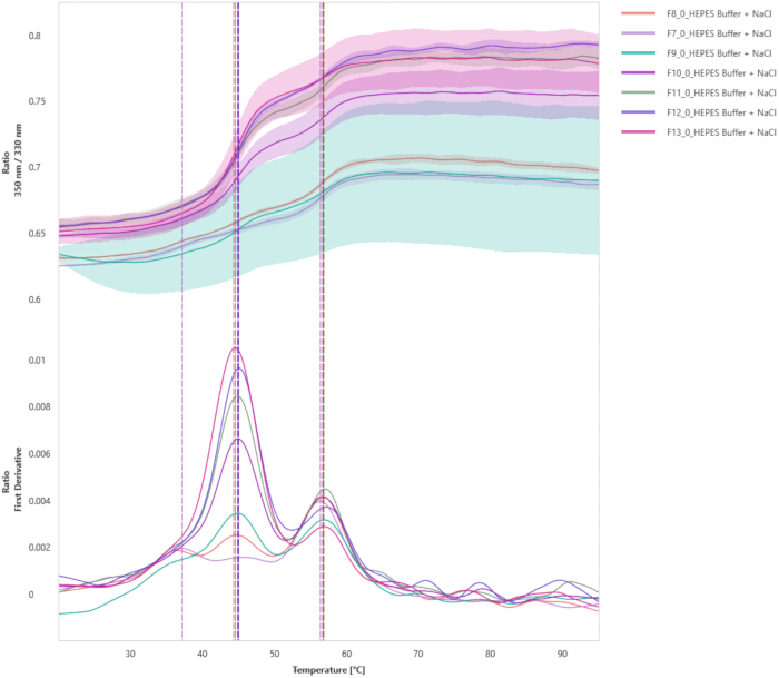
Figure 3: Differential scanning fluorimetry of purified TMEM120A M207A in LMNG. DSF reveals a thermodynamic inflection point at 46 °C, indicating the protein's thermal stability under the tested buffer conditions. Please click here to view a larger version of this figure.

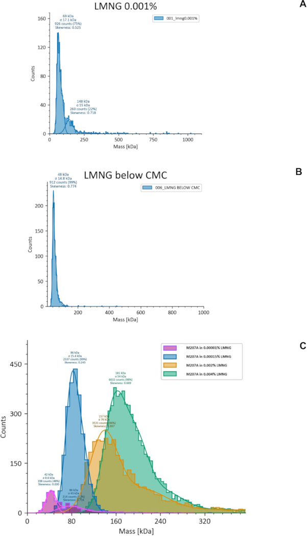
Figure 4: characterization of purified TMEM120A M207A in LMNG detergent using mass photometry technique. (A,B) Mass photometry of SEC buffer with varying LMNG concentrations. At 0.001% LMNG (above the critical micelle concentration, CMC), the apparent molecular weight is ~69 kDa, corresponding primarily to LMNG micelles. At 0.0001% LMNG (tenfold below the CMC), the peak appears at ~48 kDa.(C) Mass photometry analysis of LMNG concentration-dependent effects on TMEM120A oligomerization. TMEM120A in 0.00001% LMNG (~20x below the CMC, magenta) exhibits a main population at approximately 42 kDa (monomer). In 0.00015% LMNG (~10x below CMC, blue), a population at ~86 kDa is observed, consistent with the dimer. In 0.001% LMNG (~2x above CMC, orange), a major species at ~150 kDa corresponds to protein-detergent complexes. In 0.002% LMNG (~4x above CMC, green), a broad distribution centered at ~180 kDa indicates larger micelle-associated assemblies or higher-order oligomers. These results demonstrate that LMNG concentration strongly influences the apparent oligomeric state of TMEM120A, with monomer-dimer equilibrium observed below the CMC and protein-detergent complex formation predominating above the CMC. Please click here to view a larger version of this figure.

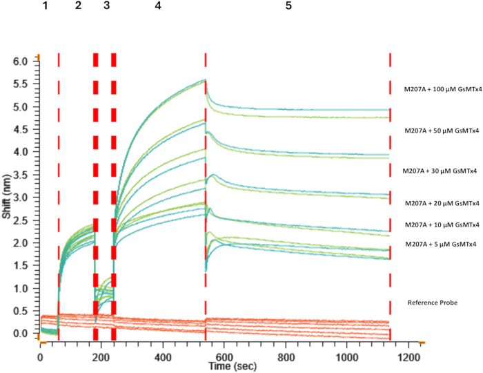
Figure 5: Raw data from software showing TMEM120A M207A-GsMTx4 interactions. Biolayer interferometry demonstrates that TMEM120A (M207A) binds the mechanosensitive channel inhibitor GsMTx4 with micromolar affinity. The figure shows the raw BLI response data obtained from Gator Prime software, delineating the five key assay phases: (1) Initial baseline, during which the signal remained stable; (2) Protein immobilization (loading), resulting in an increase of approximately 1.5 nm in wavelength shift; (3) Second baseline, allowing removal of unbound or loosely associated protein; (4) Association phase (ligand binding), where increasing GsMTx4 concentrations produced a response rise up to ~5.5 nm within 300 s; and (5) Dissociation phase (ligand release), showing gradual signal decay over 600 s. Please click here to view a larger version of this figure.

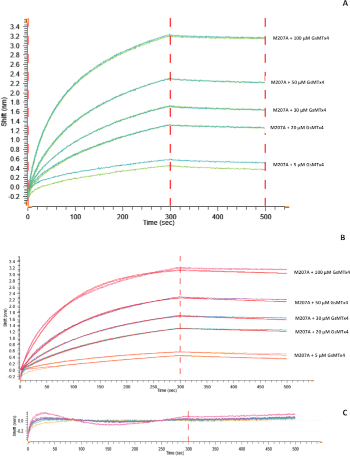
Figure 6: Binding kinetics of TMEM120A M207A with GsMTx4 peptide. (A) Association and dissociation sensorgrams of TMEM120A M207A interacting with GsMTx4 at five concentrations: 5 µM, 20 µM, 30 µM, 50 µM, and 100 µM. The 10 µM dataset was excluded from fitting due to overlap with the 5 µM curve, which improved the overall model fit. Vertical dashed red lines indicate the start and end of the dissociation phase.(B) The fitting of the sensorgrams was performed using a Local Full fitting Langmuir 1:1 association-dissociation model. Red curves represent the fitted model, while experimental traces correspond to the measured association and dissociation data for each GsMTx4 concentration (two replicates per condition).(C) Residual plots showing the deviation between experimental data and the fitted model for both association and dissociation phases, confirming the goodness of fit. Please click here to view a larger version of this figure.

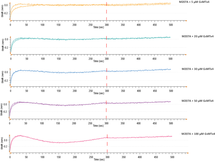
Figure 7: Residual plots corresponding to the fitted binding curves shown. Each plot represents the residuals (difference between the experimental data and the fitted model) for a single GsMTx4 concentration: 5 µM, 20 µM, 30 µM, 50 µM, and 100 µM. Residuals are displayed as shift deviation (nm) versus time (s), showing random distribution around zero across both association and dissociation phases. The lack of systematic deviation indicates a good fit of the Local Full fitting Langmuir 1:1 model for TMEM120A M207A at all tested concentrations. Please click here to view a larger version of this figure.

Table 1: Summary of kinetic parameters for TMEM120A M207A binding to GsMTx4. Kinetic parameters were obtained from Local Full fitting using a Langmuir 1:1 binding model. Association (k_on), dissociation (k_off), observed rate constants (k_obs), and equilibrium dissociation constants (K_D) are reported for each GsMTx4 concentration and replicate. Fit quality was assessed using R² and χ² values for full, association, and dissociation phases. Across all concentrations, fits showed high correlation coefficients (R² > 0.99) and low relative χ² values, indicating reliable model performance. Notes: M Conc. indicates the concentration of GsMTx4 (µM). k_obs represents the observed rate constant reflecting combined association and dissociation processes. Errors reported for k_obs, k_on, and k_off reflect fitting uncertainty. R² values indicate goodness-of-fit for full, association, and dissociation phases. Relative χ² values represent normalized goodness-of-fit metrics, while absolute χ² values indicate residual deviation between observed and fitted data. Abbreviations: k_on = association rate constant (1/M·s); k_off, = dissociation rate constant (1/s); k_obs = observed rate constant (1/s); K_D = equilibrium dissociation constant; R_max = maximum response; R_eq = equilibrium response. Please click here to download this Table.

Table 2: Processing parameters and residuals of kinetics fitting. Processing parameters: Association start, 0 s; association end, 300 s; dissociation start, 100 s; dissociation end, 300 s. Minimum R² value, 0.9; maximum χ² value, 8. Alignment step: one-step end (index = 1, average = 0). Inter-step correction was applied during the association phase. Association average, 50; dissociation average, 0. Savitzky-Golay smoothing was disabled. Please click here to download this Table.

Supplemental Figure S1: Optimization experiment for loading different concentrations of TMEM120A M207A protein on anti-FLAG probes with a fixed concentration (100 nM) of GsMTx4 peptide. (A) Raw BLI sensorgrams showing the five steps of the kinetic measurement: (1) baseline in SEC buffer or assay buffer (25 mM HEPES, pH 7.8; 200 mM NaCl; 0.00015% (w/v) LMNG; 0.0005% (v/v) Tween-20); (2) loading of four different concentrations of TMEM120A M207A onto the FLAG probe, with the reference probe (orange) used as a negative control to confirm the absence of nonspecific binding; (3) at second baseline step; (4) the association phase, and (5) the dissociation phase. (B) Global 1:1 binding model fits for the four TMEM120A M207A concentrations interacting with 100 nM GsMTx4 peptide. (C) Residual plots for both the association and dissociation phases, showing minimal deviations from the fitted model (<0.05 nm). Please click here to download this File.

Supplemental Figure S2: Plate setup and assay configuration. (A) Plate design for a 384-well plate, where different parameters can be assigned. Samples correspond to the ligand (GsMTx4) at various concentrations. Orange wells indicate TMEM120 M207A protein at 250 nM. Wells represent protein replicates at 250 nM, and the same buffer was used for baseline, association, and dissociation steps.(B) Max Plate view showing four anti-FLAG biosensor probes: one reference probe and three probes for protein replicates. All probes were pre-wetted in assay buffer, regenerated in Q buffer, and neutralized in assay buffer. The same buffer was used throughout baseline, association, and dissociation steps. Please click here to download this File.

Supplemental Figure S3: Assay setup cycles, including baseline, protein loading, second baseline, association, and dissociation. Abbreviations: B = buffer; L = load; 0, 5, 10, 20, 30, 50, and 100 = GsMTx4 concentrations in µM. Please click here to download this File.

Supplemental Figure S4: New kinetics (K) analysis workflow. Select Experiment icon, which provides an overview of all assays performed within a single experiment. Please click here to download this File.

Supplemental Figure S5: New kinetics (K) analysis workflow.Align and Filter icon, where raw data for both association and dissociation phases can be reviewed and analyzed. Please click here to download this File.

Supplemental Figure S6: New kinetics (K) analysis workflow.Set Reference icon, used to select the appropriate reference sensor for background subtraction and accurate data interpretation. Please click here to download this File.

Supplemental Figure S7: Binding fitting steps in the kinetic analysis workflow. Kinetic fitting parameter settings used for analyzing binding interaction data. The model assumes a 1:1 interaction with a single ligand binding site. The fitting type is set to Local, fitting each concentration curve independently rather than globally. The Full fitting option with Full Stitch enabled includes the entire continuous association and dissociation curves. Time windows for association and dissociation phases are set from 0 to 300 s and 0 to 200 s, respectively. In the background, the binding fitting graph, residual graph, and individual assay curves illustrate fit quality and experimental variability. Please click here to download this File.

Supplemental Figure S8: Binding fitting steps in the kinetic analysis workflow. Binding fitting graph showing association and dissociation phases across multiple assay replicates and probe positions (C1 and D1). The residual graph below assesses fit quality, with residuals indicating differences between the experimental data and the fitted model; values near zero reflect a good fit. The accompanying table summarizes fitting statistics, including Full R², Association R², Dissociation R², and Chi-square (X²) values for each replicate. Please click here to download this File.

Supplemental Figure S9: Binding fitting steps in the kinetic analysis workflow. Kinetic analysis of binding interactions from multiple replicates and probe positions (C1 and D1). The sensor response shift (nm) over time (s) displays association and dissociation phases, with each curve color-coded by assay and probe position. The vertical dashed red line marks the transition between association (0-300 s) and dissociation phases. Below, the table reports kinetic parameters derived from the 1:1 binding model fit, including analyte concentration (M Conc.), association rate constant (k_on), dissociation rate constant (k_off), errors, and the equilibrium dissociation constant (K_D). The consistent fit quality supports the robustness of the kinetic measurements. Please click here to download this File.

Supplemental Table S1: Table illustrating the symbols used in both the 384-well plate and the Max Plate. Please click here to download this File.

Supplemental Table S2: Kinetic parameters obtained for the four concentrations of TMEM120A M207A loaded onto FLAG biosensors interacting with 100 nM GsMTx4 peptide, using fixed kon and koff values. Please click here to download this File.

Discussion

Characterizing membrane protein interactions remains challenging due to the need for meticulous protein purification, careful optimization of detergent concentration, and precise assay design. This study presents a detailed workflow for TMEM120A M207A, illustrating both purification and kinetic analysis using GsMTx4 with biolayer interferometry (BLI).

Critical steps and optimization:
One of the important critical steps was detergent concentration, which was identified as a major determinant of protein stability. The purification process involved cell solubilization with a buffer containing 0.5% LMNG, followed by sequential washing with 0.005% LMNG, elution with 0.001% LMNG, and final size-exclusion chromatography (SEC) in a buffer containing 0.00015% LMNG. This detergent strategy, based on LMNG's low critical micelle concentration (CMC) and slow off rate, provided improved stability of the protein in micelles during purification. The SEC buffer contained detergent at a concentration 10-fold below LMNG's CMC (0.001%), effectively minimizing its impact on downstream biophysical assays. Protein homogeneity and the absence of aggregation were confirmed using mass spectrometry and thermal stability analysis. Figure 2, Figure 3, and Figure 4 illustrate successful optimization of purification and protein stabilization in sub-CMC detergent concentrations.

Protein immobilization on the biosensor was carefully controlled to achieve 50-80% probe saturation. A loading level of 50-80% may introduce some degree of mass transport limitation; however, this range was selected to provide adequate signal strength in the BLI system, where the probes moved between wells during the assay. Achieving this level of ligand immobilization helped maintain consistent signal quality, although such loading levels have both advantages and potential limitations. Including a reference probe was critical for BLI experiments.

An additional control experiment in which four different levels of immobilized TMEM120A were tested with a single peptide concentration (100 nM). These data are now included in the revised manuscript (Supplemental Figure S1). Increasing the amount of immobilized protein produced higher loading signals, but in all cases, the shift remained below 1 nm from the baseline (Supplemental Figure S1A). We reported the fitted association and dissociation curves using a global 1:1 binding model, and we also included the residual plots, which show small non-significant differences between the fitted and experimental data.

In the main kinetic assays (5-100 µM analyte), the fitted rate constants showed the expected concentration-dependent trends. The k_off values ranged from approximately 1.48 × 10⁻⁴ to 1.43× 10⁻³ s⁻¹, while the k_on values ranged from 1.12 × 10² to 1.26 × 10¹ M⁻¹s⁻¹. These gradual changes across the concentration series are consistent with normal analyte-dependent association and dissociation behavior.

In the control experiment, where different probe-loading levels were tested at a single analyte concentration (100 nM), all four traces yielded very similar kinetic constants. The k_off values were consistently 1.42 × 10⁻¹ s⁻¹, and the k_on values were consistently 2.76 × 10³ M⁻¹s⁻¹ across all loading levels. This lack of variation suggests that neither the association nor dissociation phases were affected by probe density, mass-transport limitations, or analyte rebinding.

It is also expected that the dissociation at 100 nM appears faster in the control experiment. The 100 nM analyte concentration is roughly an order of magnitude below the K_D, and at concentrations well below K_D the complex is less stable, and the effective occupancy is low. Under such conditions, dissociation proceeds more rapidly because the binding affinity is weaker at low analyte concentrations, and reassociation during the dissociation phase is minimal. This behavior aligns with what is typically observed when the analyte concentration is substantially lower than K_D.

Taken together, the consistency of the kinetic parameters across probe loadings and the expected behavior at low analyte concentrations support the notion that the observed rate constants reflect genuine binding properties rather than artifacts from surface loading or mass-transport effects.

Binding kinetics and interpretation:
Kinetic analysis was performed using a 1:1 Langmuir association-dissociation model with a local full-fitting strategy, in which individual analyte concentrations were fitted independently within a shared kinetic framework (Figure 6B). This approach was selected over traditional global fitting because certain datasets, particularly at lower ligand concentrations, displayed minor overlaps or early-phase deviations likely caused by mass transport limitations and detergent micelle effects on protein diffusion. Global fitting assumes that all traces strictly follow the same kinetic behavior, which can be compromised when surface accessibility or local microenvironment differs slightly between concentrations. Local full fitting allowed each analyte concentration to be modelled independently while still maintaining a consistent kinetic framework, ensuring that the derived parameters accurately reflected the behavior at each concentration. The fitted curves (red) closely matched the experimental traces, yielding an estimated dissociation constant (K_D) in the low micromolar range. Residual analysis (Figure 6C) did not reveal major systematic deviations, supporting the suitability of the model for these detergent-solubilized membrane protein interactions.

TMEM120A M207A and GsMTx4 showed K_D values in the low micromolar range (∼0.8-3.3 µM). The association rate (k_on) increased modestly with ligand concentration, whereas the dissociation rate (k_off) remained very slow, indicating stable complex formation. The initial rapid signal decay during the first 5-10 s of dissociation likely reflected readily accessible binding sites, whereas the slower phase represented more stable interactions (Figure 6A). These observations highlight the importance of carefully selecting dissociation windows and considering mass transport limitations when analyzing detergent-solubilized membrane proteins (Table 2).

Limitations and troubleshooting:
Several limitations should be considered for detergent-solubilized membrane proteins like TMEM120A M207A. Mass transport effects can occur during the early association phase, as the protein may diffuse slowly to the biosensor surface, which can slightly distort kinetic measurements. Sensor overloading is possible if probe saturation exceeds the recommended 50-80% range, potentially limiting the accuracy of global kinetic analysis and affecting kon and koff values. Detergent-dependent effects may influence protein stability, oligomeric state, or surface accessibility, especially at concentrations above or near the CMC. Additional factors include minor baseline drift, nonspecific binding, and challenges in capturing the kinetics of very slow dissociation.

Many of these issues can be mitigated by simple adjustments: reducing protein loading to avoid over-saturation, optimizing buffer composition, and including reference probes to correct baseline drift or nonspecific signals. In this study, the SEC buffer containing 0.00015% LMNG and low concentrations of Tween-20 effectively minimized nonspecific binding while maintaining protein stability. Carefully selecting the dissociation window for kinetic fitting, along with replicate measurements and residual analysis, was also important for confirming the reliability of kinetic parameters. These strategies generally enhance reproducibility and help generate more robust and interpretable data. Local full fitting was employed in place of global fitting to account for minor differences between traces at individual ligand concentrations, ensuring that kinetic parameters accurately reflected the behavior of each dataset.

BLI and other biophysical techniques:
Compared with surface plasmon resonance (SPR) and isothermal titration calorimetry (ITC), biolayer interferometry (BLI) offers several practical advantages for analyzing membrane protein-ligand interactions. Like SPR and ITC, BLI can provide detailed insights into binding interactions, including association rates (k_on), dissociation rates (k_off), and equilibrium dissociation constants (K_D), without requiring complex microfluidic systems or high protein concentration¹⁴. The open-well, dip-and-read format allows rapid buffer exchange and parallel processing of multiple samples, supporting higher experimental throughput. Unlike ITC, which requires large quantities of highly pure protein and provides thermodynamic data, BLI can measure both the rates of complex formation and dissociation from minimal sample concentration in nanomolar. BLI is also compatible with detergent- or lipid-containing buffers, making it suitable for low-yield or unstable membrane proteins that are challenging to study with other biophysical methods. Despite these advantages, complementary techniques such as SPR or ITC remain useful for confirming thermodynamic consistency and cross-verifying binding parameters under detergent-free conditions and detergent conditions but need a high protein concentration³.

Future directions:
This workflow can be extended to study other membrane proteins, protein-lipid interactions, or screening small-molecule modulators. Combining BLI with orthogonal approaches such as mass photometry, structural characterization, or cryo-EM could provide more detailed insights into oligomerization, stoichiometry, and binding mechanisms. Further optimization may also enable analysis of high-affinity ligands, multivalent interactions, or complexes in more native-like lipid environments.

In conclusion, careful control of protein immobilization, detergent concentration, and buffer conditions allows BLI to generate reliable, reproducible kinetic data for TMEM120A M207A and similar challenging membrane proteins. While inherent limitations exist, the method provides a robust platform for studying specific, moderate-affinity protein-ligand interactions under well-defined experimental conditions.

Materials

List of materials used in this article

Name	Company	Catalog Number	Comments
384-well black microplate	Greiner Bio-One	781906	BLI
Amicon Ultra Centrifugal Filter, 30 kDa MWCO	Sigma-Aldrich	UFC903008	Purification
Anti-FLAG probe	Gator Bio	160036	BLI
ANTI-FLAG M2 Affinity Gel	Sigma-Aldrich	A2220-10ML	Purification
BioRender	BioRender	https://biorender.com	Figure 1 creation
Bovine Serum Albumin	Sigma-Aldrich	9048-46-8	Mass photometry
CD 293 Medium (1x)	Thermofisher	11913019	Cell culture
Centrifuge 5920 R: Large Capacity and High Performance	Eppendorf	NA	Purification
cOmplete, Mini, EDTA-free Protease Inhibitor Cocktail	Merck	11836170001	Purification
Deoxyribonuclease I from bovine pancreas	Sigma-Aldrich	9003-98-9	Purification
ExpiFectamine 293 Transfection Kit	Thermofisher	A14524	Transfection
Gator Bio software	Gator Bio	NA	BLI
Gator Plus	Gator Bio	NA	BLI
GlutaMAX Supplement	Thermofisher	35050061	Cell culture
GsMTx4 trifluoroacetate	Sigma-Aldrich	SML3140-1MG	BLI
HEK293T/SF17 cells adapted to suspension growth	ATCC	ATCC CRL11268	Cell culture
LMNG (Lauryl maltose neopentyl glycol)	Thermofisher	A50940	Purification
Max Plate	Gator Bio	130062	BLI
Phenylmethylsulfonyl fluoride (PMSF)	Sigma-Aldrich	11359061001	Purification
Prometheus High Sensitivity Capillaries	Nano Temper	PR-C006	Thermodynamic stability
Prometheus Panta	Nano Temper	NA	Thermodynamic stability
Q Buffer (0.3% Glycine pH 3.8)	Gator Bio	120010	BLI
Qsonica Q500 Sonicator Ultrasonic Cell Disrupter	Qsonica	NA	Purification
Superdex 200 Increase 10/300 GL	Cytiva	GE28-9909-44	Purification
Synthesized TMEM120A (M207A) gene cloned into pCDNA 3.1 plasmid with FLAG-3C-Linker	GenScript Biotech	NA	Plasmid
TWEEN 20	Sigma-Aldrich	P1379-25ML	BLI
Two MP	Refeyn	NA	Mass photometry

References

- Rong, Y., et al. TMEM120A contains a specific coenzyme A-binding site and might not mediate poking- or stretch-induced channel activities in cells. eLife. 10, e71474(2021).
- Livnat-Levanon, N., Vigonsky, E., Lewinson, O. Real-time measurements of membrane protein-receptor interactions using surface plasmon resonance (SPR). J Vis Exp. (93), e51937(2014).
- Kovachka, S., Soule, P., Mus-Veteau, I. Microscale thermophoresis to evaluate the functionality of heterologously overexpressed membrane proteins in membrane preparations. Methods Mol Biol. 2507, 445-461 (2022).
- Ciesielski, G. L., Hytönen, V. P., Kaguni, L. S. Biolayer interferometry: a novel method to elucidate protein-protein and protein-DNA interactions in the mitochondrial DNA replisome. Methods Mol Biol. 1351, 223-231 (2016).
- Concepcion, J., et al. Label-free detection of biomolecular interactions using biolayer interferometry for kinetic characterization. Comb Chem High Throughput Screen. 12, 791-800 (2009).
- Apiyo, D. O. Biolayer interferometry (Octet) for label-free biomolecular interaction sensing. Handbook of Surface Plasmon Resonance. Schasfoort, R. B. N. , 2nd edn, Royal Society of Chemistry. 356-397 (2017).
- Egan, D., Slaybaugh, C., Wang, R. Getting started: kinetics assay using bio-layer interferometry. Gator Bio Technical Note. , (2023).
- Beaulieu-Laroche, L., et al. TACAN is an ion channel involved in sensing mechanical pain. Cell. 180 (5), 956-967.e17 (2020).
- Niu, Y., et al. Analysis of the mechanosensor channel functionality of TACAN. eLife. 10, (2021).
- Xue, J., et al. TMEM120A is a coenzyme A-binding membrane protein with structural similarities to ELOVL fatty acid elongase. eLife. 10, e71220(2021).
- Chen, X., et al. Cryo-EM structure of the human TACAN in a closed state. Cell Rep. 38, 110445(2022).
- Suchyna, T. M. Piezo channels and GsMTx4: two milestones in our understanding of excitatory mechanosensitive channels and their role in pathology. Prog Biophys Mol Biol. 130, 244-253 (2017).
- Wallner, J., Lhota, G., Jeschek, D., Mader, A., Vorauer-Uhl, K. Application of bio-layer interferometry for the analysis of protein/liposome interactions. J Pharm Biomed Anal. 72, 150-154 (2013).
- Wang, D. S., Fan, S. K. Microfluidic surface plasmon resonance sensors: from principles to point-of-care applications. Sensors (Basel). 16 (8), 1175(2016).
Reprints and Permissions
This article has been published
Video Coming Soon