Adaptive Quality Video Streaming Optimization: An Intelligent Multi-Neural Framework for Enhanced Quality of Experience in 5G and Beyond Networks

Summary

This article presents the AQVSO (Adaptive Quality Video Streaming Optimization) framework as an integration of advanced neural and optimization models designed to enhance video streaming in 5G and next-generation networks. The framework improves video quality, reduces buffering, and optimizes resource use.

Abstract

AQVSO (Adaptive Quality Video Streaming Optimization) is a new video streaming framework that aims to enhance video streaming quality and resource utilization in 5G & Beyond networks. The study proposes an end-to-end multi-neural network comprising four co-related modules that incorporate sparse convolutional networks with policy-driven encoders (SCN-PDE), a sparse graph attention convolutional network (SGA-ConvNet), adaptive spiking neural networks (ASNN), and deep belief networks with ant colony optimization (DBN-ACO). These elements dynamically adjust to network changes based on a mathematical model that aims to strike a balance between quality and resource use. Experiments on the UCF-101 dataset show that AQVSO preserves SSIM scores similar to those of state-of-the-art algorithms BBA and BOLA (0.977), while requiring much less bandwidth (4,936/8,000 kbps). The framework can save 38% in bandwidth consumption while maintaining high perceptual quality (PSNR = 45.89 dB) and has nearly eliminated buffering occurrences. The system achieves 99.9% streaming certainty under mobile, CDN (Content Delivery Network), and enterprise conditions, providing an actual performance gain for video delivery systems in resource-limited situations. This is made possible by providing a manageable user experience and efficient use of network resources through adaptive , content-aware streaming decisions.

Introduction

The objective of this study is to develop an integrated multi-neural adaptive streaming framework, termed AQVSO, that jointly optimizes perceptual video quality and bandwidth utilization under dynamic 5G and beyond network conditions. The method aims to unify content analysis, rate control, and resource allocation into a single decision architecture to achieve consistent Quality of Experience (QoE) at significantly lower bitrate requirements.

Adaptive Quality Video Streaming Optimization (AQVSO)

In the era of 5G and beyond, AQVSO is focusing on improving video streaming quality-of-experience (QoE) by adopting a multi-neural network-based model that intelligently balances perceptual quality and resource utilization¹. This network-aware scheduling strategy can address the challenge of providing high-quality video streams in a time-varying or unstable network environment with reduced bandwidth consumption and server congestion².

Video traffic currently accounts for over 80% of total mobile data globally in 2023, driving the need for efficient multimedia delivery systems to an all-time high³. Legacy networks are being transformed into agile, virtualized, software-based networks enabled by Software Defined Networking (SDN), Network Function Virtualization (NFV), Multi-access Edge Computing (MEC), and cloud/edge computing in the fifth generation (5G) environment^4,5. These advances enable next-generation applications with faster data rates, lower latency, and higher connection density⁶.

Given increasing levels of competition, Quality of Experience (QoE) has become one of the most important measures for service providers^7,8. QoE not only includes the traditional Quality of Service (QoS) metrics but also adds user perception and integrates objective QoS parameters with users' subjective experience factors, such as expectations, emotions, and preferences^9,10,11. With respect to multimedia services, QoE directly affects end-user satisfaction and can be regarded as a universal metric for overall quality assessment that links user experience with  application and communication system performance¹².

QoE of video streaming relies on parameters such as latency, bitrate, and visual quality. Network congestion caused by data growth and capacity limitations impairs the continuity of streaming quality^13,14. Common approaches offer variable video attributes (with distinct frame rates and resolutions), but user mobility and wireless channel variation demand more intelligent management strategies^15,16,17.

Current adaptive streaming solutions are heavily constrained in dynamic conditions. Dynamic Adaptive Streaming over HTTP (DASH) relies on client-side heuristics that can falter in unpredictable wireless environments¹⁸. There are reinforcement learning (RL)- based methods, such as Pensieve, that facilitate adaptation but are computationally expensive and require abundant training data¹⁹. Buffer-Based Algorithm (BBA) primarily considers buffer occupancy and ignores content complexity and perceptual quality²⁰. Model Predictive Control (MPC) heavily depends on bandwidth predictions, which can fail in a mobile environment²¹. BOLA (Buffer Occupancy based Lyapunov Algorithm) focuses mainly on the playback utility and does not take quality fairness into sufficient account²².

Recent advances ranging from cross-modal attention aggregation in SCA-PVNet²³, edge-enabled real-time analytics in RES²⁴, and efficient edge cloud transcoding²⁵ to hybrid denoising frameworks improving input stability²⁶ demonstrate the rapid progress in intelligent multimedia processing. Enhanced content understanding via 2D-CNN spatiotemporal learning²⁷ and transformer-based video modeling²⁸, along with adaptive bitrate control through CNN-RNN architectures²⁹, forms a strong foundation for next-generation streaming intelligence.

AQVSO goes beyond these individual advancements by unifying content analysis, perceptual modeling, and network-aware decisioning into a single integrated architecture that delivers consistently superior QoE under dynamic wireless conditions. AQVSO is fundamentally different from these schemes. In that, it integrates video encoding, network dynamics, data traffic, and resource allocation and user perceptual quality jointly in a coordinated manner. This comprehensive control scheme overcomes the shortcomings of traditional rate-adaptive methods by coordinating eight dedicated mechanisms²³.

Scope and application

The scope of AQVSO includes mobile 5G and beyond networks, CDN-assisted streaming environments, and enterprise cloud scenarios for redundancy in large-scale video delivery. The framework is developed under the assumption of distributed edge-computing nodes with lightweight inference capabilities, as in today's MEC-based 5G networks. Contextual limitations, such as computational cost imposed by neural components and reliance on precise network and QoE-state prediction, will be presented, specifying when AQVSO works best. The system is also not appropriate for ultra-low-resource environments without edge computing, or for real-time interactive applications that need sub-10ms latency.

AQVSO is composed of eight novel techniques: Adaptive Spiking Neural Network (ASNN) leveraged for content- and network-aware optimization; Rate Control Algorithm designed to adjust the bitrate in real-time; Deep Belief Network (DBN) utilized for traffic pattern forecasting; Ant Colony Optimization (ACO) exploited to address the network resource allocation problem at hand; Sparse Graph Attention Network (SGA), which models intricate relationships between video and the network topology at large scale; Sparse Convolutional Network (SCN), which processes high-dimensional data; Policy-Driven Encoder (PDE), an adaptive encoding strategy policy that leverages the learned knowledge on video trends over time, and Stream Bayes Change Point Identifier (BCPI), a filter that detects shifts from different dimensions related to networks and videos. Collectively, these strategies constitute the crux of AQVSO and provide holistic optimization across cloud, edge, and mobile networks by concurrently addressing video encoding, traffic management, resource allocation, and perceptual quality adaptation.

In summary, AQVSO delivers a unified multi-neural framework that jointly optimizes perceptual QoE, content-aware encoding, and resource allocation across 5G+ networks, achieving superior quality-bitrate efficiency.

Protocol

The software used is listed in the Table of Materials.

Dataset setup

The UCF-101³ dataset was obtained and extracted into the Videos/UCF-101 directory. Dataset integrity was assessed through checksum verification or manual playback, and any corrupted files were excluded from subsequent processing.

Computational environment

All experiments were performed in Python 3.10 on Windows 10/11 or Ubuntu 20.04+. The software environment included tensorflow==2.17.0, opencv-python, scikit-image, numpy, pandas, and tqdm. A minimum of 8 GB RAM was used, and GPU acceleration was employed when available.

Frame extraction

Video frames were read using cv2.VideoCapture(), and grayscale conversion was carried out using cv2.cvtColor. The resulting frames were stored in sequential order within the Frames directory to preserve temporal consistency.

Base feature network

A sequential convolutional neural network was employed to process the 224 × 224 grayscale frames. Convolutional, pooling, and dense layers were used, and the model was trained for five epochs with the Adam optimizer and Binary Cross-Entropy loss to establish baseline feature representations.

Bitrate allocation and compression

Pixel-level frame complexity was estimated and used to determine proportional bitrate allocation. JPEG compression with adaptive Q-values was applied, and the processed frames were saved in the Processed directory for further evaluation.

Quality evaluation

SSIM, PSNR, and MSE calculations were performed for each processed frame. The resulting metrics were compiled into CSV files, and visualization plots were generated and stored in the Output directory.

Final execution

The complete workflow was executed using framework.run(). This execution produced the final set of processed frames, metric summaries, and evaluation plots.

1. Adaptive Quality Video Streaming Optimization

1.1 System architecture overview

A method is presented here for optimizing video streaming specifically for 5G and beyond networks through the AQVSO framework. The approach combined several cutting-edge elements that complemented one another to improve QoE and maximize the use of network resources. A complex pipeline was utilized to process video streams, with each component specializing in a particular area of video optimization. Throughout the streaming process, the system ensured optimal quality maintenance and balanced processing.

1.2 Video pre-processing and initial analysis

1.2.1 Frame extraction and quality baseline

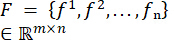
The given optimization framework was built upon the video pre-processing step, which used advanced analysis techniques to establish quality standards and prepare the video content for subsequent processing. Upon entering the system, a video stream was subjected to a thorough frame-extraction procedure that split the video into individual frames and examined temporal correlations between successive frames. This preliminary processing captured the temporal dynamics of the video and set the appropriate processing parameters for the entire stream. For an input video V, frames were extracted and processed through the following mathematical formulation:

  (1)

The frame resolution was calculated as m and the total frame count as n. Frames were extracted while preserving the video's temporal coherence to enable parallel processing in later stages. The quality baseline was established by implementing a novel fusion approach. Multiple quality metrics were combined to create a comprehensive quality assessment. The overall initial QoE was determined using the specified parameters.

  (2)

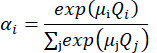
The significance of this fusion approach was considered, as it addressed the limitations of individual quality metrics. The Structural Similarity Index (SSIM) captured perceptual quality aspects that traditional metrics might have missed, while the Peak Signal-to-Noise Ratio (PSNR) provided an objective quality measurement, and the Mean Squared Error (MSE) offered a direct pixel-level comparison. The weighting factors α₁,α₂,α₃ were not static; instead, they adapted dynamically based on content characteristics. The i^th weight factor was calculated using:

  (3)

Where,

Q_i is the ith frame, i = 1,2…n

Q_j is the jth frame, j = 1,2…n, i is not equal to j

The important factors μ_i were determined through extensive empirical analysis of various video content types to ensure that the dynamic weight adjustment maintained relevant quality assessment across different types of video content and viewing conditions. Factors such as motion complexity, texture density, and the perceptual importance of different regions were considered.

1.2.2 Content complexity analysis

Content complexity was analyzed as a crucial component of the framework through a multidimensional approach that quantified various aspects of video content. This analysis was fundamental for informed decisions about resource allocation and compression parameters in later stages. A comprehensive complexity metric was introduced that considered spatial, temporal, and perceptual aspects of video content, which was given by:

  (4)

The spatial complexity component C_s(f) was calculated by analyzing the detail and texture distribution within each frame through gradient analysis. This measurement was used to identify areas that required a higher bit allocation for maintaining quality.

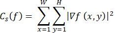  (5)

The temporal complexity component C_t(f) was calculated to quantify motion intensity between consecutive frames, as this measurement was essential for predicting compression behavior and determining appropriate buffer sizes.

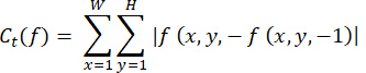  (6)

The perceptual complexity component C_p(f) integrated human vision models to prioritize regions that were perceptually significant to viewers.

  (7)

1.3 Feature extraction using sparse graph attention convolutional networks

A novel Sparse Graph Attention Convolutional Network (SGA-ConvNet) architecture was implemented in the feature extraction stage of AQVSO, marking a substantial improvement over conventional convolutional networks for video processing. The SGA-ConvNet was designed to be especially well-suited for handling high-dimensional video data in resource-constrained settings by blending the effectiveness of sparse convolutions with the adaptability of attention mechanisms. This network architecture addressed the basic problem of capturing temporal and spatial dependencies in video content. A dynamic graph was built during video frame processing, with each node representing an important feature point and edges indicating how these features related to one another. Computational overhead was significantly reduced by concentrating resources on relevant regions while preserving sparse connectivity, in contrast to conventional convolutional networks. The core operation at each layer was defined through:

  (8)

H^(l) represented the feature representations at layer l, with A ̃ denoting the normalized attention adjacency matrix. W^(l) contained the learnable weight matrices, and σ represented the non-linear activation function. The network was enabled to learn hierarchical feature representations while maintaining sparsity in the computation graph. The attention mechanism, which was crucial for adaptive feature processing, was computed through:

  (9)

α_ij represented the attention coefficient between nodes i and j, and [h_i ∣∣ h_j] denoted the concatenation of their feature vectors. The LeakyReLU activation was used to prevent vanishing gradients while preserving the network's ability to learn from negative features. The attention mechanism dynamically adjusted the importance of different feature connections based on their relevance to the current frame's content.

1.4 Dynamic rate control through adaptive spiking neural networks

Dynamic rate control was implemented in the AQVSO framework (Figure 1) via the ASNN architecture, a biologically inspired approach to managing video streaming rates. The ASNN was designed specifically to handle the temporal dynamics of video streaming while adapting to rapidly changing network conditions. This component was deemed crucial for preserving streaming quality while optimizing bandwidth usage across varying network conditions. Information was processed through discrete spikes in the ASNN, mimicking biological neural networks, which provided several advantages in terms of power efficiency and temporal processing. The membrane potential of the spiking neurons was allowed to evolve according to:

  (10)

V(t) represented the membrane potential at time t, V_rest was set as the resting potential, and τ_m was defined as the membrane time constant. I(t) was calculated from network conditions and content complexity. Adaptive noise was introduced through σ(t)N(0,1) to improve robustness. This noise term helped the network maintain stability when facing rapid fluctuations in network conditions. The rate control mechanism was implemented using a sophisticated adaptation scheme:

  (11)

R(t) represented the target bitrate, S(t) represented the spike rate of the neural network, B(t) denoted the available bandwidth, and E(t) represented the error term derived from quality metrics. The exponential term expp(-λE(t)) was used to provide smooth adaptation to quality variations while preventing oscillatory behavior in the rate control system.

1.5 Quality-driven compression optimization

A novel approach was implemented in the compression optimization stage that combined perceptual quality metrics with content-aware compression strategies. This stage was made fundamental to achieving optimal trade-offs between quality and size in the compressed video stream. A region-adaptive compression scheme was utilized that allocated bits based on both content importance and perceptual quality requirements.

  (12)

C (r,t)  represented the compression ratio for region r at time t, and C_base(r) was used as the base compression ratio determined by content complexity. Q(r,t) was defined to denote the quality factor. ϕ_i (r,t) was implemented to represent various adjustment factors, including motion intensity, edge density, and perceptual importance.

1.6 Resource allocation through deep belief networks with ant colony optimization

The resource allocation mechanism in AQVSO was configured to implement a hybrid approach combining Deep Belief Networks (DBN) with Ant Colony Optimization (ACO), establishing a novel solution to the complex problem of optimal resource distribution in video streaming systems. The learning capabilities of deep belief networks were leveraged for pattern recognition in resource usage, while the optimization strengths of ant colony algorithms were utilized for real-time resource allocation decisions. The DBN-ACO system was designed to address the fundamental challenge of balancing immediate resource requirements with long-term optimization goals in dynamic network environments. The DBN component was implemented using a hierarchical learning structure composed of multiple Restricted Boltzmann Machines (RBMs), with each layer capturing increasingly abstract patterns in resource utilization. The probability distribution of hidden unit activation was modeled through:

  (13)

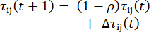
h_i represented the hidden units, v represented the visible units, b_i represented the bias terms, and W_ij represented the connection weights. This probabilistic modeling was used to capture complex dependencies in resource usage patterns while maintaining adaptability to changing conditions. The ACO component was implemented with a dynamic pheromone-based optimization strategy.

  (14)
  (15)

τ_ij represented the pheromone levels, with p serving as the evaporation rate Δτ_ij (t). was defined as the pheromone update, and η_ij represented the heuristic value based on the current network conditions and resource availability.

1.7 Adaptive buffer management and error recovery

A sophisticated buffer management system was implemented in the AQVSO framework that dynamically adjusted to varying network conditions and content characteristics. This system was designed to maintain streaming continuity while minimizing latency and preventing buffer underflow or overflow conditions. A novel adaptive approach was deployed that considered both network statistics and content complexity.

  (16)

B(t) was maintained as the target buffer size, QoE(t) was measured as the current quality of experience, σ(t) was tracked as the network stability metric, and ϕ(σ(t)) was implemented as an adaptive function to modulate buffer size based on network variability. The error recovery mechanism was executed using a multi-layered approach that combined proactive error prevention with reactive recovery strategies. A sliding window of frame references was kept within the system.

   (17)

p was used to represent the success probability of a single recovery attempt, n was taken as the number of attempts, and T(t) was applied to represent the time since error detection. This exponential decay term was used to ensure that recovery efforts were properly prioritized based on temporal relevance.

1.8 Quality assessment and feedback integration

The quality assessment system implemented a comprehensive approach that combined multiple quality metrics with user experience factors. This integration was crucial for maintaining high QoE while optimizing resource utilization. The system implemented a novel quality metric fusion:

   (18)

NB(t) was calculated as the normalized buffering ratio, SB(t) was calculated as the switching frequency, and M(t) was computed as the motion quality factor. The weights w_i were adjusted dynamically based on content type and viewing conditions.

   (19)

Θi was represented as the base weights, and f(C(t)) was applied as a content-dependent adjustment function. The feedback integration system was implemented as a closed-loop control mechanism.

  (20)

e(t) was set to represent the error between the target and achieved quality metrics, and K₁,K₂,K₃ were defined as adaptive gain parameters that adjusted based on network conditions and content characteristics.

Results

Present a thorough analysis of the performance of the proposed system and report the implementation results. Include a comparison section to confirm that the system is appropriate for Neuro Cloud Stream, a cloud-based ML approach. Figure 2 illustrates the AQVSO system workflow.

Dataset description

To evaluate the AQVSO framework, use a diverse collection of video content ranging from 10 s to 2 h and 30 min. The comprehe...

Discussion

The Adaptive Quality Video Streaming Optimization (AQVSO) framework is a multimedia processing engine based on an embedded multi-module codec integration architecture to dynamically enhance perceptual video quality and bitrate adaptivity in wireless networks. Unlike individual predictors or rate controllers, for example, AQVSO utilizes SCN-PDE to enhance motion-awareness, SGA-ConvNet for spatiotemporal attention modeling, ASNN for low-latency adaptive rate control, and DBN-ACO for globally optimized bit allocation. This ...

Materials

List of materials used in this article

Name	Company	Catalog Number	Comments
8 GB RAM	Generic		Minimum memory required for running the experiments.
Intel Core i5 Processor	Intel Corporation		CPU used for AQVSO evaluation pipeline.
NumPy	NumPy Developers		Numerical computations and matrix operations.
OpenCV-Python	OpenCV.org		Used for video loading, frame extraction, and preprocessing.
Pandas	Pandas Development Team		Data handling, CSV export, metric tables.
Python 3.10 (Programming Language)	Python Software Foundation		Required for executing the AQVSO framework scripts and dependent libraries.
scikit-image	Scikit-Image Developers		SSIM, PSNR, MSE computation.
TensorFlow 2.17.0	Google		Deep learning library used for building neural modules (SCN, SGA-ConvNet, ASNN, DBN).
tqdm	TQDM Team		Progress bars for pipeline execution.
Windows 10 (64-bit) Operating System	Microsoft Corporation		Operating system used for experiments.

References

- Barakabitze, A. A., Walshe, R. SDN and NFV for QoE-driven multimedia services delivery: The road towards 6G and beyond networks. Comput Netw. 214, 109133(2022).
- Konstantoudakis, K., et al. Serverless streaming for emerging media: towards 5G network-driven cost optimization. Multimed Tools Appl. 81 (5), 7123-7162 (2022).
- Yang, J., Bashir, A. K., Guo, Z., Yu, K., Guizani, M. Intelligent cache and buffer optimization for mobile VR adaptive transmission. Digit Commun Netw. 9 (2), 456-468 (2023).
- Guzmán, P., Arce, P., Guerri, J. C. Automatic QoE evaluation for asymmetric encoding in DASH. Ad Hoc Netw. 106, 102184(2020).
- Al-Habashna, A. A., Wainer, G. QoE awareness in progressive caching and DASH-based D2D streaming. Wirel Netw. 26 (3), 2051-2073 (2020).
- Lai, P., et al. QoE-aware user allocation in edge computing systems. Future Gener Comput Syst. 112, 684-694 (2020).
- Piran, M. J., et al. Multimedia communication over cognitive radio networks. J Netw Comput Appl. 172, 102759(2020).
- Malekzadeh, M. QoE and QoS control model for mobile video. Telecommun Syst. 77 (3), 523-541 (2021).
- Bakhati, B., et al. Modified quality video TCP-friendly congestion control. Multimed Tools Appl. 80 (16), 20907-20928 (2021).
- Chapagain, B., et al. Real-time video and path quality for tele-training. Multimed Tools Appl. 80 (8), 9615-9638 (2021).
- Laghari, A. A., et al. QoE assessment of games. Entertain Comput. 34, 100362(2020).
- Seufert, A., Schröder, S., Seufert, M. Delivering user experience over networks. SN Comput Sci. 2 (1), 1-18 (2021).
- Liu, Z., Qiao, B., Fang, K. QoE-aware encrypted video caching. J Cloud Comput. 9 (1), 1-15 (2020).
- Baccour, E., et al. RL-OPRA for resource allocation in crowdsourced video. Future Gener Comput Syst. 112, 982-995 (2020).
- Huang, G., Zhang, B., Yao, Z., Li, C. Stochastic rate control for surveillance. Comput Netw. 190, 107904(2021).
- Moura, H. D., Macedo, D. F., Vieira, M. A. Wireless QoE control using RL. Comput Commun. 154, 331-346 (2020).
- Hung, Y. H., Wang, C. Y., Hwang, R. H. Live streaming optimization in MEC. IEEE Trans Mobile Comput. 19 (4), 922-934 (2020).
- Canovas, A., et al. SDN-based multimedia traffic management. J Netw Comput Appl. 150, 102498(2020).
- Yue, T., Wang, H., Cheng, S., Shao, J. DL-based QoE evaluation. Neurocomputing. 386, 179-190 (2020).
- Felici-Castell, S., Segura-Garcia, J., Garcia-Pineda, M. Adaptive QoE cloud media architecture. Clust Comput. 22 (1), 679-692 (2019).
- Saleem, M., Saleem, Y., Hayat, M. F. QoE-aware optimization for mobile cloud. Clust Comput. 23 (2), 1381-1396 (2020).
- Zhu, Z., Tan, L., Li, Y., Ji, C. PHDFS for deep learning platforms. J Syst Archit. 109, 101810(2020).
- Lin, D., et al. SCA-PVNet: Self- and cross-attention for 3D retrieval. arXiv. , (2023).
- Ali, M., et al. Real-time video analytics on edge-enhanced clouds. IEEE Trans Cloud Comput. 10 (2), 792-804 (2022).
- Gao, G., Wen, Y. Video transcoding for ABR streaming over edge-cloud. Digit Commun Netw. 7 (4), 598-604 (2021).
- Devi, B. A., Choudhry, M. D. Hybrid denoising for IoRT video. Automatika. 65 (2), 510-522 (2024).
- Parmar, P., Morris, B. HalluciNet spatiotemporal representation. Signals. 2 (3), 604-618 (2021).
- Video transformer without convolutions. Zhang, Y., et al. Proc IEEE/CVF Int Conf Comput Vis, , 13577-13587 (2021).
- Darwich, M., Bayoumi, M. Bitrate adaptation with CNN-RNN. Clust Comput. 27, 6355-6375 (2024).
Access restricted. Please log in or start a trial to view this content.