A Computationally Efficient Hybrid Approach for Electrocardiogram-Based Arrhythmia Prediction

Summary

The model in this study is built to classify early arrhythmias in electrocardiogram (ECG) datasets from several databases into five main heartbeat types. Compared to other models, this model performs better in terms of accuracy, sensitivity, precision, and recall.

Abstract

Cardiovascular diseases, especially arrhythmias, are a leading cause of death worldwide. This highlights the need for automated systems that can detect and diagnose these conditions early. This research introduces a deep learning model that identifies arrhythmias using electrocardiogram (ECG) signals. The model focuses on five main types of heartbeats: Normal (N), Left Bundle Branch Block (L), Right Bundle Branch Block (R), Atrial Premature Beat (A), and Premature Ventricular Contraction (V). The system uses Lead I signals from several databases, including MIT-BIH Arrhythmia, Supraventricular, INCART 12-lead, and Sudden Cardiac Death Holter. This provides more than 3.9 million training segments and 112,575 testing segments.

The data is preprocessed by dividing it into fixed windows of 180 samples, scaling it using Min-Max normalization, and balancing the classes with the Synthetic Minority Over-sampling Technique. The model combines 1D Convolutional Neural Networks to extract spatial features and transformer layers to capture time-based patterns. It uses the Adam optimizer and includes dropout and batch normalization to enhance performance. The system achieves 99.99% accuracy, precision, and F1-score across all classes, which is better than the TN4 model and other top-performing models. The use of Convolutional Neural Networks and deep hybrid architectures improves the robustness of features. This model shows great potential for scalable and real-time arrhythmia detection and contributes to the advancement of AI-driven, personalized digital healthcare.

Introduction

Cardiovascular disease is the most significant cause of human health issues, with more than 17 million deaths every year. Nearly three-quarters of all cardiovascular disease (CVD) cases live in low- income countries of the world, as stated by the World Heart Federation. An electrocardiogram (ECG) captures the electrical activity generated by the heart's depolarization. The electrical signals propagate to the skin. ECG signals convey at least two pieces of vital information. One is health-related biomedicine. The other is person-related credentials or biometrics. Because of its simplicity, various methods for classifying ECG signals have been considered, including homemade and machine learning approaches. The manual method is time-consuming and inefficient. It requires real-time signals like ECG and significant computer infrastructure. Machine learning approaches are likely to yield lower bracket accuracy than the manual method, but a suitable algorithm is needed to reduce the risk of undetected arrhythmia¹.

The most common cardiovascular disease is arrhythmia, a condition in which the heartbeat pattern is abnormal. These abnormal patterns must be categorized into classes because this kind of information can impact treatment. ECG is widely used to detect abnormal heart patterns and predict heart disease, enabling early detection. The diagnosis of arrhythmia largely relies on the ECG, an important medical device used to record cardiac excitability, transmit signals, and monitor recovery. ECG is necessary and dependable in modern medicine. The automation of ECG signal interpretation greatly enhances clinical practice and improves patient safety. Arrhythmias are abnormal heart rhythms and patterns. Artificial intelligence, particularly machine learning, is an excellent tool for disease prediction and opinion analysis, especially for cardiovascular diseases².

Different medical data, such as patient records, are generally used in hospitals for clinical purposes. Medical data can also be generated in a timely manner to support the optimization of machine learning algorithms. The machine is trained on a dataset that eventually learns from it. Once trained, it can identify and classify whether a case is healthy or based on different attributes of their records^3,4. Machines can also detect patterns in the given data, which may not be easily perceived by humans due to a lack of time or limited resources. Several methods have been employed to classify ECG signals, including K-nearest neighbors (KNN), support vector machines (SVM), neural networks (NN), decision trees, linear discriminant analysis (LDA), and Bayesian classifiers. SVM is considered one of the most effective supervised learning algorithms for classifying ECG signals to detect arrhythmias^5,6.

A well-performing bracket model using NN and the multilayer perceptron (MLP) is better than other conventional methods. Deep learning algorithms such as artificial neural networks (ANNs) have been successfully employed in tasks such as information retrieval, image recognition, object detection, and language processing. CNNs have been widely used in research to extract stylistic features from ECG waveforms and dissect these features for various purposes, such as the discovery of the QRS complex and the ST segment or P waves^7,8. The 1D CNN learns to detect the most relevant features in ECG signals and classify them into five arrhythmia types. A baseline-wandering and high-frequency noise removal filter was applied to improve signal quality. This classified arrhythmias into five categories^9,10.

As shown in Figure 1, the P wave, QRS complex, and T wave are important parts of an ECG. The P Wave represents atrial depolarization, the electrical activity that causes the atria to contract. The QRS complex reflects ventricular depolarization; it is the electrical impulse that triggers ventricular contraction. The T wave indicates ventricular repolarization, the recovery phase of the ventricles after contraction. Together, these waves represent one complete cardiac cycle. They are vital for understanding how the heart works and for diagnosing heart problems¹¹.

All these waves represent one cardiac cycle. They are highly important for understanding how the heart works and for diagnosing cardiac conditions. Deep learning models have lately achieved significant strides in computer-aided medical signal interpretation, including ECG signals. Traditional hand-crafted feature-based machine learning models suffer from scalability and adaptation issues across different patient populations. To address these challenges, deep models such as CNNs and hybrid models combining CNNs with recurrent models like LSTMs have emerged to automatically learn relevant features from raw ECG signals. This has greatly improved classification accuracy¹².

This study proposes a deep learning framework for classifying ECG signals into five categories of heartbeats: Normal (N), Left Bundle Branch Block (L), Right Bundle Branch Block (R), Atrial Premature Beat (A), and Premature Ventricular Contraction (V). To train the model, we utilize publicly available ECG datasets such as the MIT-BIH Arrhythmia Database and the Supraventricular Database. These datasets are preprocessed and divided into fixed-length segments for analysis. Since class imbalance is a common issue in arrhythmia data, we apply the Synthetic Minority Over-sampling Technique (SMOTE) to balance the training data. This ensures the model can learn effectively from all classes and improve its accuracy in classifying different types of heartbeats.

Drawing inspiration from recent progress in ECG classification, including models using continuous wavelet transforms (CWT) and CNN architectures, the proposed approach employs both a standard CNN and a hybrid model incorporating transformer layers. By combining a CNN for spatial feature extraction and a transformer for capturing temporal dependencies, this system achieves high accuracy, with F1 and precision close to 100% across all classes^13,14.

"Spatial features" refer to traits related to the position or location of something, such as distance, direction, and shape. On the other hand, "temporal features" describe elements related to time, like when an event occurred, its duration, or the sequence of events. Essentially, "spatial" means "space" and "temporal" means "time."

The main goals of this research were to develop an accurate, scalable model for real-time arrhythmia detection and to support the expanding field of AI-driven diagnostics in healthcare. This system shows promise for real-time monitoring, enabling early detection and intervention for patients at risk of cardiac events.

The aims of this research work are multifaceted. First, this proposed technique aims to classify arrhythmic beats into five categories: normal (N), left bundle branch block (L), right bundle branch block (R), atrial premature beat (A), and premature ventricular contraction (V). Second, this research aims to construct a hybrid CNN and transformer model that can learn both morphological and temporal information from ECG signals without preprocessing¹⁵. Third, this proposed technique aims to provide a performance-oriented solution that can be implemented in real time. Fourth, this research will aim to demonstrate improvements in accuracy and sensitivity of the proposed model compared with state-of-the-art models^16,17.

Additionally, Graph Convolutional Networks (GCNs), which model interactions among physiological factors within a structured graph, have been introduced for biomedical prediction tasks and may play a role in future arrhythmia classification models that consider interlead dependencies.

Protocol

Ethical statement
This study relied entirely on public, anonymized ECG data downloaded from PhysioNet. All datasets used in this study were originally collected with the subjects' consent and with ethics approval from the respective data owners. This research did not require any data gathering, experimental work with either human or animal subjects, or patient personal identity information. Hence, no additional ethics review was requested.

Methodology
Figure 2 illustrates the workflow of the proposed architecture.

Data gathering
ECG data is collected from the PhysioNet Database, a popular repository of physiological signals. Multiple datasets are retrieved from the database. These datasets are merged into a single main dataset that includes various ECG signal classes.

Datasets used
This study used several publicly available ECG datasets to develop and evaluate a deep learning model for arrhythmia classification. The selection of these datasets was done with care, considering their diversity in terms of patient demographics and the variety of arrhythmia types, to ensure that the proposed model performs well across different scenarios⁹. For this study, only Lead-I data from the MIT-BIH Arrhythmia Database, the MIT-BIH Supraventricular Arrhythmia Database, the St. Petersburg INCART 12-lead Arrhythmia Database, and the Sudden Cardiac Death Holter Database were combined. These datasets are known for their high-quality, annotated ECG recordings that encompass a broad spectrum of arrhythmia classes.

The combined datasets above include patient demographics, recording devices, sampling frequencies, and settings. The above-mentioned variability in the model improves its generalization by exposing it to a wide range of ECG morphologies, noise, and rhythms.

Datasets description
MIT-BIH arrhythmia database
The MIT-BIH Arrhythmia Dataset has 48 half-hour ECG recordings, numbered 100-234. Each record contains two-channel ECG signals digitized at 360 samples per second. Data is stored in .dat, .hea, and .atr formats.

MIT-BIH supraventricular arrhythmia database
This is a specific subset of the MIT-BIH databases. The MIT-BIH Supraventricular Arrhythmia Database includes 78 full-length ECG recordings, ranging from 30 min to several hours, numbered 801-811. Each record includes two-channel ECG signals, converted to digital form at 128 samples per second.

The St Petersburg INCART 12-lead arrhythmia database
This database includes 75 annotated recordings taken from 32 Holter monitors. Each recording lasts 30 min and includes 12 standard leads, each sampled at 257 Hz. The signal strength varies between 250 and 1100 analog-to-digital converter units per millivolt.

Unforeseen cardiac death Holter database
This dataset is one of the many open- access Holter recordings that capture factual occurrences of ventricular tachycardia (VT) and ventricular fibrillation (VF). Both can lead to unforeseen cardiac death. Each record is 24 h long and sampled at 250 Hz.

Data preprocessing
In this study, four public ECG databases with different sampling rates were used: MIT-BIH Arrhythmia (360 Hz), MIT-BIH Supraventricular Arrhythmia (128 Hz), St. Petersburg INCART 12-lead (257 Hz), and Sudden Cardiac Death Holter (250 Hz). To ensure all data were consistent and could be combined during model training, all ECG signals were resampled to a common rate of 360 Hz, which matches the MIT-BIH Arrhythmia Database and is commonly used as a standard in ECG research. Resampling was performed via band-limited interpolation; initially, the ECG signals were low-pass filtered to prevent aliasing, and subsequently, a sinc-based reconstruction kernel was used for interpolation, followed by final resampling at 360 Hz. After resampling, each signal was divided into windows of 180 samples, roughly equivalent to 0.5 s of data, ensuring all datasets had the same time resolution. This standardization enabled combining signals from different databases for training and testing, helping the model learn consistent patterns over time.

Preprocessing involved several important steps to ensure input data quality:
Data segmentation:
After resampling, each ECG signal was divided into fixed-length windows of 180 samples. This corresponds to about 0.5 s of signal duration at a sampling rate of 360 Hz. This research used a fixed, non-overlapping sliding window for segmentation. Each window collected a continuous sequence of ECG samples. The study chose a 180-sample window because a 0.5 s interval is enough to capture a full cardiac cycle or its main parts: the P wave, QRS complex, and T wave, for typical adult heart rates. A class label was assigned to each segment based on the annotation in the center of the segment. This way, the segment label matched the main heartbeat shape within that window. sliding window method, applied this segmentation function:

where s_i is the ECG sample at time i.

Normalization:
Normalized the segmented ECG data with Min-Max scaling to make sure all features had values between 0 and 1¹⁰.

This step helps speed up the model's convergence during training.

Class balancing with SMOTE
Normal (N) beats greatly outnumbered abnormal heartbeat classes in the ECG dataset, which showed a significant class imbalance. After segmentation, normalization, and train-test splitting, the training dataset was subjected to the Synthetic Minority Over-sampling Technique (SMOTE) to address this problem.

A 180-dimensional feature space was used to represent each ECG segment, consisting of 180 normalized samples. SMOTE used the Euclidean distance to determine each minority-class sample's k nearest neighbors (k = 5) within its own class. SMOTE was applied only to the training data, which was split into 70% training and 30% test sets using stratified sampling. This way, no artificial samples were added to the testing set, ensuring that the test results were not influenced by the oversampling process. The test data remained unchanged, preserving its original class distribution, and was used only to evaluate the model fairly. As a result, the high performance results from this study demonstrate the model's true ability to generalize, not due to overfitting or inflated scores from adding extra samples.

Train-test split:
After preprocessing and class filtering, the dataset was divided into training and test subsets at a 70%–30% split using stratified random sampling. This stratification is based on the class labels to ensure the relative proportions of each heartbeat class are maintained in the training and test sets.

The split was performed using a random seed for reproducibility. Every ECG segment appeared exclusively in either the training or the testing set. To avoid bias and data deviation, every preprocessing step that might affect data distribution (namely, class balancing via SMOTE) was performed only after splitting and solely on the training data.

In this regard, by maintaining class proportions, using random stratification, and strictly separating samples into training and test sets, the splitting process reduces the likelihood of bias in the samples, allowing performance metrics to reflect the model's generalization rather than data-specific residuals.

Dataset splitting and class distribution
The final dataset was split into training and test sets, with 70% for training and 30% for testing. After applying SMOTE, the class imbalance was reduced, ensuring that each arrhythmia type was well represented in both the training and test sets. A total of 3,966,620 ECG segments were used for training, while 112,575 ECG segments were used for testing. The large volume of data, combined with the variety of arrhythmia types, enabled the creation of a model that effectively identifies different arrhythmia types in real-world ECG signals. This study uses deep learning models to classify ECG arrhythmias. The five heartbeat types, namely Normal (N), Left Bundle Branch Block (L), Right Bundle Branch Block (R), Atrial Premature Beat (A), and Premature Ventricular Contraction (V), were chosen in keeping with the standardized beat annotations provided in the MIT-BIH Arrhythmia Database as well as AAMI guidelines for ECG beat annotation. All five beat annotations mentioned here encompass significant heart conditions that fall within the broad category of arrhythmias and exhibit distinctive waveform features in the ECG signals around the P, QRS, and T waves.

Moreover, these classes are among the most frequent and consistently labeled in public ECG databases, making it easier to test their effectiveness compared with other ECG-based heart rhythm classification approaches. The datasets were split using a cross-patient method. This setup ensured that ECG segments from a single patient would not appear in both the training and testing sets simultaneously. Once that split occurred, SMOTE was applied only to the training set. The test set remained free of synthetic samples and repeated temporal windows. All of this helps avoid segment-level overlap and supports true generalization when dealing with patients not previously seen.

Class distribution before and after SMOTE:
The original dataset had a significant imbalance between classes, with a large number of Normal (N) beats and fewer samples for the abnormal classes. Before using SMOTE, the training data had around 133,320 Normal (N), 8,075 Left Bundle Branch Block (L), 10,431 Right Bundle Branch Block (R), 4,489 Atrial Premature Beat (A), and 60,682 Premature Ventricular Contraction (V) segments. To address the imbalance, SMOTE was applied only to the training set, increasing the number of samples in the minority classes to match the majority class. After the augmentation, each class had 793,324 segments, resulting in a total of 3,966,620 ECG segments for training. The test set, which had 112,575 segments, kept its original class distribution and was not oversampled. This approach ensured a fair and unbiased evaluation of the model's performance.

Training and inference
looked at computational efficiency by checking the training and inference performance on an NVIDIA RTX 3050 GPU with 6 GB of memory. The training process took around 3.2 h for 60 epochs. Inference latency came in at an average of 0.45 ms for every 180-sample segment, which makes real-time use possible. Memory usage on the GPU hit a peak of 4.2 GB, and the model only has 1.8 million parameters, so it feels lightweight next to most transformer-based ECG setups.

The training and inference process has the following steps:
Training setup: Training parameters, such as learning rate, batch size, and epochs, are defined.
Model training: The CNN-Transformer model is trained on the training data.
Validation: After training, the model's validation accuracy and loss are checked. If performance is good, the model is saved. If performance is poor, the pipeline repeats with different training parameters, going back to the parameter setting step.

Model architecture
The whole CNN-Transformer setup has four main parts: convolutional feature extraction, a projection layer, the transformer encoder, and finally the classification head. The convolutional block begins with a one-dimensional convolutional layer with 32 filters, a kernel size of 3, a stride of 1, and padding of 1, followed by a ReLU. It reduces things with max-pooling, kernel size 2, to cut down the temporal resolution of the signal. After that first convolution layer, there is another one with 64 filters, same kernel size 3, stride 1, padding 1, ReLU again, and another max-pooling with size 2. The output from all this is flattened, passed through a linear projection layer that maps features to a 128-dimensional embedding space, which then feeds into the transformer^18,19.

The transformer block has two encoder layers, each with multi-head self-attention using 4 heads to capture long-range dependencies in the ECG signal. In each layer, there is a position-wise feedforward network with a hidden size of 256 and dropout at 0.5 to help with overfitting. Layer normalization occurs after each sublayer, which stabilizes training.

For the classification head, it's a fully connected layer that drops from 128 to 64, followed by ReLU and dropout 0.5 again. Then the output layer has five neurons for the arrhythmia classes, with Softmax to get probabilities.

1D Convolutional Neural Network (CNN) blocks:
The CNN block consists of two 1D convolutional layers, each followed by a ReLU activation and a max pooling layer. These layers help identify spatial relationships within the input ECG signal. To enhance feature extraction, additional ReLU activation functions are applied after each transformation step in the CNN layers.

First convolutional layer: This layer uses 32 filters, each of size 3, on the input signal. The process can be written as:

      

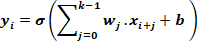
where y_i is the output, w_j represents the weights of the filter, x_i+j is the input segment, b is the bias term, and σ represents the activation function (ReLU). The resulting feature map goes through a ReLU activation layer to add non-linearity:

Pooling layer: After each convolutional operation, a max-pooling step is applied to reduce the spatial dimensions by half. This process is defined as:

This helps in retaining the most significant features while also reducing the computational load.

Second convolutional layer: This layer uses 64 filters of size 3 x 3 to process the feature maps from the previous layer, allowing the model to detect more complex patterns. After the convolution, a ReLU activation function is applied to introduce non-linearity into the model.

This step ensures that the model captures detailed patterns from the ECG signal.

Additional activation layers: ReLU activation is applied after each step following the convolution process to help the network better capture complex patterns, ensuring the model focuses on positive activations.

Flattening process: After the second max-pooling operation, the feature maps are flattened into a single vector for input to the transformer block.

Transformer blocks:
The transformer block consists of two layers of multi-head self-attention, which help the model understand the relationships between different parts of the ECG signal over time. Multi-Head Self-Attention works by looking at every pair of elements in a sequence. For a sequence with query Q, key K, and value V, the attention is calculated as:

Here, dk is the dimensionality of the key vectors, ensuring scale invariance.

Feedforward layers: Each self-attention output goes through a fully connected feedforward network with ReLU activation, followed by layer normalization. This step refines the extracted temporal features:

where W1 and b1 are the weights and biases of the feedforward layer.

Batch-first representation: The transformer operates on sequences in a batch-first layout, ensuring compatibility with the CNN block's input format.

Fully connected (dense) layers:
After processing through the transformer block, the output sequence is flattened and then sent through two fully connected layers to carry out the classification. The first fully connected layer transforms the input vector into a 128-dimensional feature space, reshaping it in the process.

where W is the weight matrix, x is the input vector, and b is the bias vector. A ReLU activation layer is applied:

A dropout layer with a rate of 0.5 follows to prevent overfitting.

Second fully connected layer: The final layer maps the 128-dimensional features to the number of heartbeat classes (e.g., 5 classes for arrhythmia detection). The output goes through a log-SoftMax function to compute the log probabilities: exp(xi)

Hybrid CNN-Transformer model
The model presented is a Hybrid deep learning model that combines the strengths of CNNs and transformers to use both spatial and temporal representations. Such architecture is specially adapted for processing complex, long-sequence data such as physiological signals.

The equation represents the input representation, where N = number of samples, T = number of time steps, d = feature dimension per time step.

This equation signifies the positional embeddings, where pos = position in sequence; i = embedding dimension index.

CNN module – Local feature extraction
CNNs learn efficiently local dependencies and morphological patterns such as peaks, slopes, or spikes in sequential data. The convolutional layer uses  kernels of spatial extent  over an input tensor . Each output channel m is determined by:

 = number of input channels; K = size of the kernel; W = filter weights; b = bias

ReLU function
In this case, represents the learnable weight and  is the bias for channel mA, nonlinear activation, like the Rectified Linear Unit (ReLU), is applied:

Pooling and feature compression
Pooling layers reduce the spatial or temporal dimension of feature maps, preserving important features and reducing computation. In max pooling with window size  and stride s, the pooled feature at location  is:

Output length after pooling

Where  ​ is input length; stride defines a step size for sliding the pooling window. This formula computes the output length of a feature map after a pooling operation (e.g., max pooling). It calculates how much the feature map is downsized based on input length, pool size, and stride. Transforms multidimensional feature maps into a vector for fully connected layers.

Transformer encoder – capturing long-range dependencies
Transformers use self-attention to learn long-range temporal dependencies in sequences¹⁷.

Scaled dot-product attention

Q, K, V are query, key, and value matrices calculated through learned projections;  is the key dimension used to scale the dot product.

Multi-head attention

 Each head computes attention independently; outputs are concatenated and linearly transformed.   are learned projection matrices for each head.   is the final projection weight after concatenation^18,19_.

Final prediction and loss
Fully connected layers map features to logits, which are then transformed into predictions using activation functions. After some convolutional and pooling layers,  is flattened into a vector  A fully connected layer computes the logits: A fully connected layer then computes the class logits:

Sigmoid/Softmax activation:

The activation function maps the model's raw output `z` to probabilities. Sigmoid is applied to binary classification, and Softmax for multi-class problems for the distribution of probability across classes. z is the linear output (e.g., last layer: z = Wx + b). Output ŷ is between (0, 1), which signifies probability²⁰.

Training process
The training was performed on a system with the following hardware specifications:
Processor: AMD Ryzen 7 7840HS
CPU RAM: 16 GB
GPU RAM: 6 GB NVIDIA GeForce RTX 3050

The models were trained using the Adam optimizer, which adapts the learning rate during training based on the first and second moments of the gradient. The update rule for Adam is given by:

In this setup, m^t and v^t represent the first- and second-moment estimates, α is the learning rate, and ε is a small constant used to prevent division by zero. The models were trained for 60 epochs, with early stopping to prevent overfitting. A batch size of 1024 was used, and the training data was loaded into the models using PyTorch's DataLoader. Dropout and batch normalization were incorporated to regularize the model and accelerate convergence. Dropout is a regularization method that randomly turns off a percentage p of the neurons during training, which helps reduce overfitting. Mathematically, let zi denote the activation of the i^th neuron. During the training phase, the modified activation z' is calculated as:

where p is the dropout rate (e.g., p = 0.5 for a 50% dropout). During inference, no dropout is applied, and the full network is used.

Convergence in neural networks is a problem that significantly impacts existing classification systems in the healthcare sector, especially when diagnoses are inconsistent due to insufficient convergence. Recent research on predefined-time optimization approaches and convergence at a fixed time has shown that it is still possible to train models that converge within a fixed number of iterations for all initial states. Future models based on this one can include predefined-time optimization.

Batch normalization:
Batch normalization stabilizes and accelerates training by normalizing the inputs to each layer. Given a mini-batch of activations x = {x₁, x₂, . . ., x_N}, the batch-normalized output x_i .is computed as:

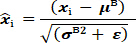
where µ^B and σ^B2 are the mean and variance of the batch, ϵ is a small constant for numerical stability, and γ and β are learnable parameters that scale and shift the normalized values. Batch normalization helps reduce internal covariate shift and enables the use of larger learning rates. These techniques, combined with the Adam optimizer, ensure robust training by mitigating overfitting and improving convergence speed^21,22.

Figure 3 shows Validation Loss and Validation Accuracy over Epochs during the training of a machine learning model. The validation accuracy (blue line, right Y-axis) starts relatively low (about 97.5%) and increases quickly within the first 10 epochs. It continues to improve and reaches levels of around 99.7% to 99.8% after about 20 epochs. This indicates that the model is learning and applying knowledge well on the validation set. The validation loss (red line, left Y-axis) starts high, then drops sharply to nearly zero within the first few epochs (around 2 to 3). After that, it stays flat at nearly zero for the rest of the training^23,24.

Results

This section introduces a hybrid deep learning model designed to categorize arrhythmias from ECG data. The model is evaluated on its ability to recognize five clinically significant heartbeat classifications: Atrial Premature Contraction, Normal, Left Bundle Branch Block, Right Bundle Branch Block, and Premature Ventricular Contraction. Comprehensive assessment is essential given the clinical relevance of these arrhythmia classes and the challenges posed by imbalanced datasets and signal variability.

Discussion

In recognizing and categorizing arrhythmias from ECG bio signals, the proposed deep learning hybrid model combines transformer structures and 1D Convolutional Neural Networks (CNNs) and shows excellent performance. This combination takes advantage of the transformer's ability to learn global time dependencies through self-attention mechanisms and the CNN's capability to identify localized spatial features from raw ECG waveforms. The model was tested using five important heartbeat classes: Normal, Left Bundle Bran...

Materials

List of materials used in this article

Name	Company	Catalog Number	Comments
Adam Optimizer	Open-source (PyTorch)	https://pytorch.org/docs/stable/optim.html	Optimization algorithm used to train the deep learning model by adapting learning rates during backpropagation.
Hardware (Computational System)	AMD; NVIDIA	https://www.amd.com/en/products/processors/laptop/ryzen/7000-series/amd-ryzen-7-7840hs ; https://www.nvidia.com	Processor: AMD Ryzen 7 7840HS; CPU RAM: 16 GB; GPU: NVIDIA GeForce RTX 3050 (6 GB VRAM). Used for model training and evaluation.
Imbalanced-learn	Imbalanced-learn	https://imbalanced-learn.org	Python library used for class balancing with Synthetic Minority Over-sampling Technique (SMOTE).
Matplotlib	Matplotlib	https://matplotlib.org	Python library used for plotting ECG signals, confusion matrices, and performance graphs.
PhysioNet ECG Databases	PhysioNet	https://physionet.org	Public ECG datasets used in the study, including MIT-BIH Arrhythmia, MIT-BIH Supraventricular Arrhythmia, INCART 12-lead, and Sudden Cardiac Death Holter databases.
PyTorch	PyTorch	https://pytorch.org	Python deep learning framework used to implement CNN and Transformer models, training pipeline, and inference.
Python	Python Software Foundation	https://www.python.org	Programming language used for data preprocessing, model development, training, and evaluation.
Seaborn	Seaborn	https://seaborn.pydata.org	Python data visualization library used for statistical plots and result visualization.
WFDB	WFDB	https://wfdb.readthedocs.io	Python package used for reading, writing, processing, and plotting physiological signals and annotations from PhysioNet databases.