Explainable Federated Learning Model for Cross-Institutional Digital Financial Data Collaboration and Risk Control

Summary

We demonstrate a reproducible protocol for implementing FedRisk, an explainable federated learning framework. The procedure includes semantic data harmonization, privacy-preserving entity alignment, differential privacy calibration, local GBDT training, global Transformer fusion, and gradient-compressed asynchronous updates, enabling secure, scalable, and regulation-compliant financial risk prediction across multiple institutions.

Abstract

The fragmentation of financial data across institutions and stringent privacy regulations severely hinder collaborative risk management, leading to suboptimal fraud detection with accuracy below 60% and high SME loan default errors exceeding 25%. Existing federated learning solutions face challenges with Non-IID data, model interpretability, and compliance, resulting in real-world adoption rates below 20%. To address these gaps, we propose FedRisk, an explainable federated learning framework integrating four key innovations. First, a cross-institutional data mesh with ontological semantic harmonization achieves feature utilization above 85%. Second, a hybrid AI model combines locally interpretable GBDT with monotonic constraints and a global attention-based Transformer, reducing performance loss in Non-IID scenarios by 7.6% compared to FedAvg. Third, a tripartite privacy mechanism employs adaptive differential privacy with a total budget of ε=5, additive secret sharing, and fairness-aware regularization, limiting group prediction bias below 0.05 and RAROC loss under 2.1%. Fourth, communication-efficient optimizations reduce per-round bandwidth to 8.5 MB and training time to 85 min. Evaluated on over 5 million multi-institutional records, FedRisk achieves an AUC-ROC of 0.912, only 1.8% lower than centralized GBDT, while resisting membership inference attacks with an AUC of 0.58. It reduces cross-institutional data transmission by 99% and outperforms classic FL baselines by 7.3% in AUC-ROC. By enabling secure, transparent, and regulation-compliant risk prediction without raw data sharing, FedRisk provides a scalable solution for cross-institutional financial collaboration.

Introduction

The in-depth development of digital finance is reshaping service models, from personal credit risk control to SME supply chain financing, establishing data as a core production factor. According to the PBOC's "2023 China Fintech Development Report", by late 2023, China's digital credit scale exceeded 65 trillion yuan, accounting for 38% of the total balance, with daily transaction data surpassing 500TB¹. However, "data silos" remain a significant barrier. Institutions generally adopt closed data models due to competition and security concerns. For instance, in credit card fraud detection, banks relying solely on internal data miss critical cross-institutional records, resulting in identification rates below 60% for new fraud types. Similarly, for SME credit, the lack of external insurance and tax data leads to default prediction errors exceeding 25%. This fragmentation causes dual challenges: limiting access for 200 million underserved clients and increasing risk cross-contagion by 18% (CBIRC 2023 Report). Consequently, data silos have become the core bottleneck hindering the high-quality development of digital finance.

In recent years, a surge in global data privacy laws has significantly limited centralized data sharing. Financial institutions must now adhere to three core principles: "minimum necessity," "informed consent," and "traceability." While regional frameworks vary, they all impose stringent thresholds on cross-institutional data usage, as detailed in Table 1.

Regulatory framework	Core restrictive clauses	Impact on financial data collaboration
EU's General Data Protection Regulation (GDPR)	1. Cross-border data transfer must meet the "sufficiency determination"; 2. Individuals have the right to access and delete their data; 3. Data breaches must be reported within 72 hours	Unauthorized cross-border transmission of raw data is prohibited, and centralized sharing requires a privacy impact assessment (PIA), increasing compliance costs by 30%
California Consumer Privacy Act (CCPA)	1. Consumers can ask companies to delete their personal data; 2. Data sharing requires clear notification of what it will be used for	Centralized platforms require data access interfaces for each consumer, increasing operational costs by 25% and making it easy for consumers to delete data and cause missing training data for the model
China's Personal Information Protection Law	1. Personal information processing requires separate consent; 2. Sensitive personal information processing requires additional authorization documents; 3. Establish a "data classification and protection" system	Cross-institutional data sharing requires authorization from each customer, and the authorization rate is less than 40% in practice. Centralized mode is difficult to implement
EU Payment Services Directive II (PSD2)	1. Open the bank data interface; 2. Data sharing should be based on customer authorization and limited use	Although it supports data sharing, it requires that the whole process of interface access be tracked, and the centralized platform should assume the responsibility of interface security and audit, which significantly increases the technical complexity

Table 1: Comparison of core requirements of major data regulatory frameworks.

This study introduces three pivotal innovations to address challenges in cross-institutional federated risk modeling. First, a data mesh architecture with an ontological semantic layer standardizes heterogeneous schemas, achieving over 85% feature utilization while preserving data sovereignty. Second, a hybrid AI model combines locally interpretable GBDT with regulatory-compliant monotonic constraints and a global attention-based Transformer. By dynamically weighting institutional outputs, this model reduces Non-IID performance loss by 7.6% while maintaining an AUC-ROC of 0.912. Third, a tripartite privacy-compliance mechanism integrates adaptive differential privacy (ε=5), additive secret sharing, and fairness-aware regularization to ensure GDPR compliance, limit ΔDP bias to < 0.05, and resist membership inference attacks (AUC=0.58). Together, these innovations reconcile the demands of data fragmentation, regulatory interpretability, and privacy-security tradeoffs in federated financial AI.

Federated learning in finance is categorized into Horizontal Federated Learning (HFL)², Vertical Federated Learning (VFL)³, and Federated Transfer Learning (FTL)⁴ based on data distribution (Table 2).

Federal paradigm	Core features	Financial risk control adaptation scenario	Representative studies	Boundedness
Horizontal federal learning	The data feature space of the participants is consistent, but the sample space is different	Cross-organizational credit card fraud detection	McMahan et al. [[i]](2017) proposed the FedAvg algorithm, which for the first time applied HFL to financial anti-fraud by achieving cross-institutional model collaboration through parameter averaging, and improved the fraud detection rate by 12% on a 10-bank data set	Without considering the non-independent and identically distributed (Non-IID) characteristics of financial data, when the difference of customer risk distribution between institutions exceeds 30%, the AUC-ROC of the model decreases by more than 15%
Vertical federal learning	The sample space of participants is consistent, but the feature space is different	Collaborative credit risk control between banks and insurance companies	Yang et al. [[ii]] (2020) proposed the SecureBoost algorithm, which achieves vertical feature joint training through homomorphic encryption, and achieves a default prediction accuracy rate of 89.3% in the small and micro business loan scenario	It relies on strict entity alignment , which has high risk of privacy leakage, and the training efficiency drops sharply when the feature dimension is too large
Federal Transfer Learning	There are differences in data distribution and feature space of participants	Cross scenario risk migration	Pan et al.[[iii]] (2021) solved the problem of sample scarcity in supply chain finance by initializing the parameter migration optimization model, which improved the convergence speed by 60%	"Negative migration" is likely to occur during the migration process. When the risk mechanism difference between the source scenario and the target scenario exceeds 40%, the model performance exceeds the traditional model
[[i]]McMahan, B., Moore, E., Ramage, D., Hampson, S., & y Arcas, B. A. (2017). Communication-efficient learning of deep networks from decentralized data. Proceedings of the 20th International Conference on Artificial Intelligence and Statistics, 1273–1282.
[[ii]]Yang, Q., Liu, Y., Chen, T., & Tong, Y. (2020). Federated machine learning: Concept and applications. ACM Transactions on Intelligent Systems and Technology, 10(2), 1–19.
[[iii]]Pan, S. J., & Yang, Q. (2021). A survey on transfer learning. IEEE Transactions on Knowledge and Data Engineering, 33(12), 2345–2359.

Table 2: Comparison of learning paradigms in the financial sector.^5,6,7

Recent advances address scenario-specific challenges: FedSSL⁸ tackles label scarcity through contrastive learning, while FedLite⁹ achieves 490× communication reduction for resource-constrained institutions. Extensions to healthcare¹⁰, security vulnerabilities¹¹, multimodal finance¹², and scalability¹³ demonstrate FL's broad applicability.

Privacy protection is central to financial risk control. The three mainstream techniques-Differential Privacy (DP)¹⁴, Secure Multi-Party Computation (SMC)¹⁵, and Homomorphic Encryption (HE)¹⁶-offer distinct advantages in strength, efficiency, and adaptability. DP is formally defined by Pr[M(x) = y] ≤ e^∈ ⋅ Pr[M(x') = y] + δ, where M represents the randomized algorithm, $x$ and $x'$ denote neighboring datasets, and y is the algorithm output. This ensures output similarity across datasets, strictly limiting individual leakage through controllable noise. A comparative analysis of their technical characteristics is presented in Table 3.

Type of technology	Core principles	Privacy strength (ε value)	Computation complexity	Financial scenario adaptability
Differential privacy	Individual contributions to the data set are indistinguishable by adding noise	ε=1-5 (recommended value for financial scenarios)	O (n) (n is the sample size)	High, suitable for the whole process of model training, can be seamlessly combined with federated learning
Secure multi-party computing	Multiple participants collaborate to compute without disclosing intermediate results	Information-theoretic security	O (n²) (vertical federal scenario)	Yes, it is suitable for sensitive feature joint calculation, but it takes too long in large sample scenarios
Homomorphic encryption	The encrypted data is calculated directly and the correct result is obtained after decryption	Computationally secure	O (n³) (based on lattice cryptography)	Low, only suitable for small-scale parameter transmission , millions of samples scenario calculation time more than 24 hours

Table 3: Comparison of privacy protection technology characteristics.

In financial applications, differential privacy has become the mainstream choice due to its "privacy-effect balance control". Dwork, C.¹⁷ proposed the classic (ε, δ)-DP definition, providing a quantitative standard for privacy protection. The core formula is as follows:

  (1)

Here M As a privacy protection algorithm, D and D is an adjacent data set (only one sample difference), Privacy budget (the smaller the privacy protection, the stronger), r Privacy budget (the smaller the privacy protection, the stronger), δ The probability of failure (usually taken 10^-5).

Abadi, M. et al.¹⁸ developed Differential Privacy Stochastic Gradient Descent (DP-SGD), utilizing gradient clipping and noise injection to reduce credit risk model privacy leakage to below 8%. Secure multi-party computation (SMC) and homomorphic encryption are primarily employed for sensitive processing. For instance,Bogetoft, P. et al.¹⁹ applied SMC to cross-bank credit scoring, ensuring only final scores were accessible. Perri, L.² proposed a fully homomorphic encryption algorithm for secure parameter aggregation, though high computational complexity limits its application to small-scale training among medium-sized banks.

AI risk control models have evolved from traditional centralized architectures to distributed architectures, with two paradigms showing significant differences in data dependency, performance, and compliance costs. Centralized models include Gradient Boosting Trees (GBDT) and deep learning models. The GBDT algorithm proposed by Friedman, J., Hastie, T.Tibshirani, R.²¹ enhances risk prediction accuracy through multi-tree integration, achieving an AUC-ROC of 0.93 in personal credit scenarios. However, it requires collecting complete customer data, posing risks of data breaches and compliance challenges. Zhang, H., Liu, Y., Zhang, X., Yin, Z.Li, Y.²² developed a transformer-based risk control model that improves fraud detection rates by 15%, yet its parameter size exceeds 10 GB. The distributed paradigm includes parameter-sharing and feature-sharing approaches. Parameter-sharing (e.g., FedAvg) aggregates local parameters but struggles with Non-IID characteristics: AUC-ROC dropped from 0.89 to 0.82 as default rate differences rose from 0.5% to 3.5%. Feature-sharing (e.g., SecureBoost) enables vertical collaboration but requires precise alignment, with performance plummeting by 20% when errors exceed 5%.

The core of federated learning is to enable multi-institution collaborative training without raw data transfer. This framework defines the participants, training process, and objective function. In this study, the system consists of Kfinancial institution nodes (denoted as P₁, P₂, ..., P_K) and a coordinator C. Each institution P_K holds a local dataset 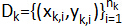, X_k,i∈R_d which are the customer feature vectors y_k,i∈{0,1}, for risk labels (0 is normal, 1 is defaultfraud), local sample size, full data scale . The training follows a "local iteration-global aggregation" process: i) Initialization: The coordinator generates initial global parameters θ₀ and distributes them to all institutions; ii) Local iteration: in the round of training, the institution P_K is based on local data and current global parameters θ_t, minimizing the local loss function through gradient descent, get the updated local parameters θ_t,k, that is:

 (2)

Where n is the learning rate and ∇_θL_k(θ_t) is the gradient of the local loss a θ_t  is the gradient of the local loss a θ_t; iii) Global aggregation: Institution encrypts and uploads local parameter to the coordinator, the coordinator generates new global parameters θ_t+1 by sample size weighted aggregation:

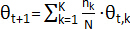 (3)

iv) End condition: Repeat step 2-3 until the global model's performance on the validation set does not improve for successive rounds, Output the final model. θ^* = θ_T. Given the non-independent identic distribution (Non-IID) characteristics of financial data, it is necessary to extend the assumptions of traditional federated averaging (Fed AvgP_k). This study employs dual dimensions of "label distribution heterogeneity" and "feature distribution heterogeneity" to characterize Non-IID: Let the proportion of positive instances (default events) in institutions be defined as:

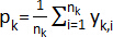 (4)

Define the tag isomorphism coefficient ; Let the mean difference of set features be ,When α>0.03 and when, It is determined to be a high Non-IID scenario.

According to the attacker's ability and target, the threat scenarios are divided into three categories, as shown in Table 4

Type of threat	Attackers identity	punching bag	Typical means
A semi-truthing attack	Participating institutions/ coordinators	Infer customer characteristics of other institutions	Gradient inversion and member reasoning attacks based on model parameters
hostile attack	Malicious institutions	Pollution global model	Upload false gradients and poison models
External attack	Unauthorized third parties	Steal parameters/features in transit	Intermediate attacks, eavesdropping on communication links

Table 4: Threat model classification of the Financial System.

Using (ε,δ) -Differential privacy (Differential Privacy, DP) as the core privacy protection standard, its essence is to add noise so that the influence of "whether the data set contains a sample" on the model output can be ignored. The formal definition is as follows: For federated learning M algorithms, If for any two adjacent datasets and that differ only by one sample (DΔD' = 1), As well as any output S⊆Range(M) set, it satisfies:

Pr[M(D)∈S]≤e^ε⋅Pr[M(D^')∈S]+δ  (5)

Then it is called satisfied (ε,δ)-DP. One is the "privacy budget" (The smaller the privacy protection, the stronger it is , and the financial scenario is usually taken ), δ for the "probability of failure" (Generally δ≤10^-5 to ensure that low probability events do not affect privacy and security). In order to adapt to the multi-round iteration characteristics of federated training, the total privacy consumption is calculated by using the combination theorem of "Renyi differential privacy" (RDP). Let the privacy budget of each training round be ε_t, then the total privacy budget after the training of the cycle satisfies:

   (6)

This theorem provides a theoretical basis for adaptive noise calibration by dynamically allocating the privacy budget per round.

FedRisk employs a rigorous (ε, δ)-differential privacy (DP) framework, dynamically allocating privacy budgets via the Rényi DP (RDP) composition theorem. It defines global sensitivity Δf as the maximum L1-norm change in model parameters induced by adjacent datasets (differing by a single sample), with variance-aware Laplace noise calibration (noise coefficient κ_t proportional to data distribution fluctuations). Under the total privacy budget constraint ε=5 (meeting GDPR compliance thresholds), RDP converts multi-round training privacy consumption into (ε, δ)-DP (δ=10⁻⁵), balancing protection strength and model utility-empirical results demonstrate this suppresses member inference attack AUC to 0.58 while maintaining risk prediction AUC-ROC at 0.912.

The optimization of financial risk control models must simultaneously satisfy three regulatory requirements: "predictive accuracy", "privacy protection", and "fairness". Traditional optimization functions that solely aim for loss minimization are no longer applicable. A multi-objective optimization framework needs to be established to transform regulatory constraints into quantifiable regularization terms. For binary classification scenarios (default/normal), log loss (LogLoss) is adopted as the base loss function to measure the deviation between model-predicted probabilities and actual labels, defined as:

   (13)

Where p_k,i = σ(θ;x_k,i) is the predicted default probability of the sample (x_k,i,y_k,i) for the model, σ(⋅) is the Sigmoid activation function.

The requirements of GDPR, Personal Information Protection Law, and other regulations are transformed into three types of regularization terms, which are combined with the basic loss function to form the final optimization objective:

   (14)

The definition and function of each regularization term are as follows: i) Privacy constraints: Based on the noise addition cost of differential privacy, the influence of quantitative privacy protection on model accuracy is discussed. Let the global sensitivity of model Δparameters be (that is, the maximum change of parameters caused by adjacent data sets), then:

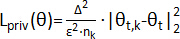   (15)

This term ensures that the added noise intensity matches the privacy budget and avoids excessive sacrifice of model accuracy. Ii) Fairness constraint: In view of the "anti-discrimination" requirements in the Personal Information Protection Law, the prediction bias of different groups is constrained. Take "demographic parity" (DemographicParity) as an example, let the positive gprediction rate of the set be 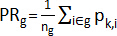, then:

(16)

This term minimizes the difference in prediction rate between different groups and avoids model discrimination. Iii) Robustness constraints : In response to the requirements of "model anti-interference capability" in Basel III, Ensure that small perturbations of the data do not significantly affect the model output. By adding adversarial sample Δx perturbations (satisfying |Δx|_∞≤γ), the research define:

   (17)

The robustness of the term enhancement model to abnormal data is improved and the risk of misjudgment is reduced. In this formula, is the regularization coefficient, it was determined by cross-validation (in this study λ₁=0.01,λ₂=0.05,λ₃=0.02), Ensure a balance between the three regulatory objectives and the accuracy of the forecast.

Protocol

System architecture

Cross-institutional data mesh and semantic layer

To address cross-institutional data heterogeneity, the research constructs a Data Mesh architecture through domain-driven node partitioning. Each financial institution operates as an independent data domain node while maintaining ownership and control rights, with the semantic layer enabling unified data comprehension and interaction. The ontology-based semantic layer establishes a unified financial risk control data model, defining core entities ,f_map attributes, and entity relationships. Specific semantic mapping rules are detailed in Table 5. For institution-specific fields, standardized conversions are achieved through semantic mapping functions:

  (18)

Kernel entity	The A field name of the institution	Name of field B in the institution	Semantic layer uniform field name	Data type	Standardized rules
Client	Premium customer rating (1-5)	VIP customer levels (bronze to diamond)	Customer credit rating (1-5)	Integer	Bronze→1, Silver→2, Gold→3, Platinum→4, Diamond→5
Business	Transaction amount (ten thousand yuan)	Transaction amount (yuan)	Transaction amount (yuan)	Floating number	The value of the A field in the institution is 10,000 times
Credit application	Applicant quota (credit ratio)	Expected loan amount	Applicant loan amount (yuan)	Floating number	Institution A: Total credit × ratio of application amount; Institution B: direct mapping

Table 5: Core entity semantic mapping rules in the field of financial risk control.

Here is x_i,j the i-th specific field value of institution j, min(x_j) and max(x_j) are the minimum and maximum values of the field within the institution, respectively, U_j and L_j define the upper and lower limits of the unified value range for this field at the semantic layer.

Blockchain-based global model registry and audit trail

To resolve issues of chaotic model version management and untraceable training processes in federated learning, blockchain technology is employed to establish a global model registry and audit - tracing system. Utilizing a consortium blockchain architecture, participating nodes include financial institutions, federated coordinators, and regulatory bodies, ensuring data immutability and multi - party consensus²³. The global model registry stores core metadata of models, including version numbers, training H_v rounds, lists of participating institutions, structural parameters , and performance metrics . This metadata is stored using a Merkle tree structure, with each model version corresponding to a unique hash value:

   (19)

Here v is the model version number, T is the total number of training rounds, S is collection of institutions participating in the training, ID_i is the unique identifier of an institution i, θ_v is the model parameter vector for the version v, and AUC_v is the AUC-ROC value of this version of the model is shown.

Federated feature engineering pipeline

Secure entity alignment and schema harmonization

Feature engineering serves as the core component of cross-institutional data collaboration, requiring effective extraction, alignment, and aggregation of features while ensuring data privacy. This study designs a comprehensive pipeline encompassing secure entity alignment, schema coordination, and differential privacy-embedded transaction graph aggregation to address both cross-institutional feature heterogeneity and privacy leakage risks²⁴. Cross-institutional entity alignment is essential for achieving feature collaboration. However, directly transmitting customer identifiers would compromise privacy. Therefore, the research adopts a privacy-preserving entity alignment method combining homomorphic encryption (HE) with locality-sensitive hashing (LSH) technology. Institutions preprocess customer identifiers using SHA-256 hash functions to generate preliminary identifiers. These identifiers are then mapped into the same "bucket" through LSH to reduce subsequent encryption computation. Identifiers within the same bucket undergo Paillier homomorphic encryption. The encrypted identifiers are uploaded to the federated coordinator, which achieves entity alignment by comparing encrypted identifiers' similarity using cosine similarity.

   (20)

When the similarity is greater than the preset threshold (in this study, it is taken as τ=0.95), it is determined to be the same entity, and a unified entity ID across institutions is generated to achieve secure entity alignment.

Differentially private aggregation of transaction graph embeddings

Financial transaction data exhibits distinct graph-structured characteristics (with clients as nodes and transactions as edges). Transaction graph embedding effectively captures clients 'related-party transaction patterns, providing critical features for risk control models. However, direct aggregation of cross-institutional G_i=(V_i,E_i)V_iiE_ie_i,_v∈R^dd transaction graph embeddings may leak clients' transaction-related information. Therefore, DifferentialPrivacy (DP) technology is introduced to achieve privacy-preserving aggregation of transaction graph embeddings. Each institution locally constructs a transaction graph, where represents the set of client nodes for the institution and represents the set of transaction edges (edge weights equal to transaction amounts). The GraphSAGE algorithm is employed to generate node embeddings (with 256-dimensional embedding dimensions in this study). To meet differential privacy requirements, Laplacian noise is added to the local embeddings:

   (21)

Here Δ_G Global sensitivity of GraphSAGE algorithm (estimated by experiment in this study Δ_G=0.8), for the local privacy budget of the agency,

   (22)

For the total privacy budget of the system, this study takes ε_total=1.5). The coordinator aggregates the noise embedding of each institution by using a weighted average strategy, with weights based on the percentage of customers of each institution:

   (23)

The aggregated global transaction graph is embedded and fed back to each institution, As a key input feature of the risk control model, it not only retains the cross-institutional transaction correlation information, but also protects customer privacy through differential privacy.

(24)

Hybrid AI risk model

Local sub-models: Gradient boosting with monotonic constraints

Traditional centralized AI risk control models struggle to adapt to cross-institutional federated scenarios. This study develops a hybrid AI risk model combining "local submodels + global fusion model", integrating the high interpretability of Gradient Boosting Trees (GBDT) with Transformer's adaptability to non-independent and identically distributed (NID) data. An interpretation module is introduced to balance model performance and explainability in federated environments. Each institution locally constructs GBDT submodels, chosen for their strong structural data fitting capability and high interpretability - essential requirements for financial risk control regulations . To prevent overfitting and illogical conclusions , monotonic constraints are implemented during GBDT training, enforcing monotonic increasing or decreasing patterns for key features like customer income and credit scores. The first tree set by GBTD is h_t(x), and the model output is:

   (25)

Here, η is the learning rate (this study takes η=0.1). Monotonic constraint is realized by loss function regularization x_j.

Add constraint term:

   (26)

Here, x≺x^' represents that the eigenvalue of x is smaller than the eigenvalue of x^', and the final loss function is:

   (27)

Here, l is the logarithmic loss function (used in the binary risk control y_i∈{0,1} scenario, indicating whether the customer defaults). is the complexity regularization term for the tree, λ and γ are the regularization coefficient (This study was conducted through λ=0.01 γ=0.5 cross-validation, n_i is the number of local samples for the institution i,T is number of trees(This study took T=100).

Global fusion: Attention-based transformer for Non-IID adaptation

Cross-institutional data exhibits significant Non-IID distribution characteristics. Traditional FedAvg algorithms, which simply average local model parameters, struggle to adapt to Non-IID data. To address this, the research introduces an attention p_i(x)=σ(F_i(x))σF_i(x)ia_i-based Transformer model for intelligent fusion of local submodels. The global fusion model takes as input the output probabilities from each institution's local submodel (sigmoid function outputs from institutional GBDT models). The Transformer architecture comprises an encoder and an attention layer, where the attention layer calculates attention weights from different institutions' outputs to achieve adaptive weighting. The attention weights are computed using Scaled Dot-Product Attention:

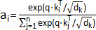   (28)

Here, q is the query vector (generated by the average risk features of global samples), is the key vector of the institution i, d_k is the dimension of the key vector (in this study d_k=64) ,n is number of agencies participating in the federation.

The final output probability of the global model is:

   (29)

Through the attention mechanism, the global model can automatically assign higher weight to the institutions with high data quality and accurate risk prediction, and improve the adaptability to Non-IID data.

Explainability module: SHAP on federated trees + counterfactual generator

Financial risk control models must maintain interpretability to satisfy regulatory requirements and protect customers 'right to know . To address this, the research develops an interpretability module combining federated SHAP+ counterfactual generators. For local GBDT submodels, the research employs SHAP values to measure feature importance, which S_i∈R^Ni^×mm quantify quantify each feature's contribution to prediction outcomes. In federated scenarios, directly transmitting local SHAP values could compromise feature distribution information. Therefore, the research implements a secure aggregation strategy where each institution locally computes the SHAP value matrix (for feature count), applies differential privacy noise) to the SHAP values, and uploads them to the federated coordinator. The coordinator then calculates the global SHAP values:

   (30)

Here, S_i^'  is the SHAP value matrix of the institution i, and w_i is the proportion of sample size of institutions.

Enter the customer's current eigenvector x and target risk rating  y_target, The output is an antifactual x_cf feature vector, satisfied (the θ_target probability threshold corresponding to the target risk rating). And |x_cf-x|₂  the minimum (i.e., the lowest adjustment cost). The loss function of the fact generator is:

   (31)

Here α,β,γ are the weight coefficients (in this study α=10,β=5,γ=1),L_GAN The adversarial loss function is used for GAN to ensure the rationality and authenticity of the counterfactual feature vector.

Privacy and security layer

Secure aggregation with additive secret sharing

In federated learning, the transmission and aggregation of local model parameters is a key link in privacy leakage. AdditiveSecretSharing (ASS) technology is adopted to achieve secure aggregation and avoid the direct acquisition of local model parameters of each organization by the coordinator. The specific process is as follows: i) Each institution will split the local model parameters into secret shares θ_i,1,θ_i,2,...,θ_i,n , satisfying , Here is the number of participating institutions; ii) The institution i sends the share θ_i,k to the institution (k≠i), keep their own share θ_i,i; iii) Each institution k collects shares sent by all other institutions θ_1,k,θ_2,k,...,θ_n,k , and sum it up with the θ_k,k share retained by itself, get the partial sum ; iv) All institutions will S_k upload and share some of it to the coordinator, the coordinator computes the global parameter aggregation results . Through additive secret sharing, the coordinator can only obtain global aggregated parameters and cannot n-1ttt=⌈n/2⌉t deduce any individual institution's local parameters. Even collusion among multiple institutions cannot recover parameters from others, ensuring privacy and security during parameter transmission. To address share loss caused by institutional disconnections, the Shamir secret sharing mechanism is introduced as a backup. Each share is further divided into fragments. By collecting any fragment, the complete share can be restored, thereby enhancing system robustness.

Adaptive noise calibration under ( ε, δ)-DP budget scheduling

The core challenge of differential privacy lies in balancing privacy protection strength with model performance. Traditional fixed-noise addition methods struggle to adapt to scenarios where data distributions dynamically change during federated training. This study designs an adaptive noise calibration mechanism based on (ε,δ)-DP, combined with a privacy budget scheduling strategy, to achieve dynamic adjustment of noise intensity. Define the total privacy budget of the system as (This study takes δ_total=10^-5 , complies with the GDPR requirements for privacy risk), Adopt the segmented budget scheduling strategy, The total budget is allocated by {ε₁,ε₂,...,ε_T} training cycle as follows, satisfied:

   (32)

In each round of training, the noise intensity is dynamically adjusted according to the distribution characteristics of local data . Assuming the local data feature variance of the t-th round of institution is , Define the noise adjustment coefficient α_i,t:

   (33)

When α_i,t≥0.8 (data distribution is stable), using a small noise intensity ; When αi,t<0.8(data distribution fluctuates) , increase the noise intensity .Among them, is the global sensitivity of the model parameters (this study ensures through gradient clipping).

Communication-efficient training protocol

Asynchronous client updates with staleness control

Cross-institutional federated learning faces challenges such as high communication latency and significant bandwidth consumption (particularly for small and medium-sized financial institutions with limited network resources). This study designs an efficient communication training protocol incorporating asynchronous client updates, gradient compression, and error feedback to reduce communication costs and enhance system scalability²⁵. Traditional synchronous federated training methods like FedAvg require waiting for all clients to complete local training before parameter aggregation, resulting in lengthy training cycles. The asynchronous client update mechanism allows clients to independently complete local training and immediately upload parameters. Upon receiving these parameters, the federated coordinator updates the global model in real-time without waiting for other clients. This addresses the model stale issue in asynchronous training . Introducing the staleness control strategy, define the staleness value for client ,(For t_current the current global training round, t_{last_update} The round in which the client last obtained the global model). When (S_max is the maximum allowable staleness, this study takes s_max=5) . The client participates in training normally; At s_i>s_max  that time, the client needs to download the latest global model again before local training. The hardware configuration consists of Intel Xeon E5-2678 v3 CPUs (12 cores, 2.5GHz) paired with NVIDIA Tesla V100 GPUs (16GB VRAM) and 64GB DDR4 memory per node to handle distributed training workloads efficiently. For software initialization, PySyft commands such as hook = sy.TorchHook(torch)andvirtual_worker = sy.VirtualWorker(hook, id="client1")are used to establish secure federated connections, while federated_train_loader = sy.FederatedDataLoader(dataset.federate((client1, client2)), batch_size=32)enables federated data loading across participants. Semantic mapping transforms financial features across institutions-for instance, converting transaction amounts from USD to CNY using a dynamic exchange rate formula:transaction_amount_CNY = transaction_amount_USD exchange_rate + (0.001 randn()), where exchange rate is periodically updated via API. To augment imbalanced datasets, CopulaGAN generates synthetic adversarial samples with a code snippet like from sdv.tabular import CopulaGAN; synthesizer = CopulaGAN(epochs=50); synthesizer.fit (train_data); synthetic_samples = synthesizer.sample(num_rows=1000), preserving statistical properties of the original data. Local GBDT training enforces monotonic constraints (e.g., ensuring "credit_score" positively correlates with "approval_probability") viaparams = {"monotonic_constraints": (1, 0, -1)}in LightGBM, while Transformer fusion is implemented in PyTorch with multi-head attention layers:self.attention = nn.MultiheadAttention (embed_dim=64, num_heads=4); attn_output, _ = self.attention(query, key, value, key_padding_mask=padding_mask), followed by layer normalization and residual connections for stability. Differential privacy injects Laplace noise scaled to the L1 sensitivity (Δf) and privacy budget (ε)-e.g., adding noise sampled from np.random.laplace(loc=0, scale=Δf/ε)where Δf=1.2 and ε=0.5-to gradients before aggregation. Fairness constraints are applied post-training by reweighting samples inversely proportional to their group prevalence (sample_weight = 1 / group_counts[y_train]) to mitigate demographic parity violations. At the same time, the weighted aggregation strategy is used to adjust the weight of client parameters according to the staleness value:

   (34)

Where λ=0.1 is the staleness penalty coefficient; the larger the staleness, the smaller the weight, which reduces the impact of stale parameters on the global model.

Gradient compression and error-feedback accumulation

Model parameters (particularly the attention weights in Transformer global fusion models) have high dimensional complexity. Direct transmission would consume excessive bandwidth, necessitating gradient compression techniques to reduce data transfer²⁶. This study integrates Top-K sparsification with quantization compression, following these specific steps: i) Top-K sparse: For the local model ∇θ_i gradient, Select the gradient element K% with the largest absolute value to retain, K The rest of the elements are zero, The value is dynamically adjusted according to the bandwidth condition (when bandwidth is sufficient K=30, when bandwidth is limited K=10); ii) Quantization compression: The retained gradient elements are quantized from 32-bit floating point to 8-bit integers. The quantization formula is:

   (35)

  

iii) Error feedback: Store the discarded gradient Δ∇=∇θ_i-∇θ_i^compressed error during compression on the client side, In the next gradient calculation, the error is accumulated into the new gradient, approach,  , Compensate for compression losses. The effects of gradient compression and error feedback are shown in Table 6, In, 8 K=20% -bit quantization conditions, The compression ratio reaches 15:1 (original data volume/compressed data volume), and through error feedback, the AUC-ROC of the model only decreases by 0.5%-1.0%, realizing the balance between communication cost and model performance²⁷.

Compression strategies	Reduction ratio	Upload bandwidth consumption (MB/ round)	AUC-ROC decline rate	Training time reduction rate
uncompressed (32-bit floating-point)	1:01	128	0.00%	0.00%
Top-30% sparse+16-bit quantization	6.7:1	19.1	0.30%	35.20%
Top-20% sparse + 8-bit quantization	15:01	8.5	0.80%	58.70%
Top-10% sparse + 8-bit quantization	30:01:00	4.3	2.10%	72.10%

Table 6: Performance comparison of gradient compression strategies.

Fairness-aware regularization

Financial risk control models must avoid discrimination against specific groups and comply with regulatory requirements including the Personal Information Protection Law and Fair Credit Reporting Act. This study introduces a fairness-aware regularization mechanism to constrain inter-group prediction biases during model training, ensuring model fairness. Two core fairness indicators are defined: i) Demographic Parity (DP): The positive prediction rate is equal for different groups, approach, , Among g them, is the group identifier ; ii) Equal Opportunity (EO): The true positive rate is equal across groups, approach . Add fairness regularization terms to the loss function of the hybrid AI risk model, and impose constraints on the local GBDT sub-model and the global Transformer model respectively: iii) Local model fairness constraints:

Here PR(g=A) is the positive prediction rate for the group g, λ and is the regularization coefficient for fairness.

iv) Global model fairness constraint: Add group fairness weight adjustment to the Transformer attention layer, the model output for vulnerable groups a_g=a_base×(1+β⋅Δ_unfair)  is given a higher attention weight, Here, Δ_unfair represents the fairness bias between this group and the dominant group(Δ_unfair=PR (dominant group)-PR (vulnerable groups)); λ_EO is the deviation compensation coefficient. The effect of fairness perception regularization is evaluated by ΔDP (DP deviation), ΔEO (EO deviation) and group calibration error .

Model governance and compliance dashboard

Real-time bias monitoring

To meet the requirements of financial regulation on model lifecycle management , the research has developed a model governance and compliance dashboard that integrates real-time deviation monitoring and regulatory reporting APIs, enabling full-process supervision and traceability throughout model training, deployment, and iteration. The real-time deviation monitoring module achieves dynamic tracking of model fairness and performance through the following dimensions: i) Group deviation monitoring: Categorizing groups by customer gender, age, region, income level, etc., calculating PR, TPR, and FPR (False Positive Rate) for each group hourly. Deviation alerts are triggered when inter-group PR differences exceed 0.08 or TPR differences exceed 0.05; ii) Performance drift monitoring: Continuously computing metrics such as AUC-ROC and PR-AUC. When these metrics decline by more than 2% consecutively over three hours, it is determined as performance drift, automatically initiating the model retraining process. iii) Privacy compliance monitoring: Record the privacy budget consumption and noise addition ε_total/10  intensity of each round of training. When the ε consumption of a single round exceeds, pause the training and adjust the noise strategy. iv) Monitoring data is displayed through visual dashboards, enabling regulators and participating institutions to view it in real time, and realizing transparent management of model risks.

Regulatory reporting API

To simplify the regulatory reporting process, a standardized regulatory reporting API is designed to support the automatic generation of reports compliant with regulations such as GDPR, CCPA, and China's Personal Information Protection Law. Core functions include: i) Data Source Compliance Report: Automatically aggregates data types, volumes, and authorization status of participating institutions to verify compliance with the "minimum necessary" principle; ii) Model Training Compliance Report: Records training iterations, participating institutions, privacy protection measures, and fairness metrics to generate a model training traceability report; iii) Risk Prediction Compliance Report: Displays regulatory-compliant distribution patterns of model predictions across different groups and counterfactual explanation cases to demonstrate non-discrimination. The API adopts a RESTful design style, supporting JSON and XML format outputs. Regulatory authorities can directly access report data through API interfaces or set automatic reporting cycles to achieve automated and standardized regulatory processes. The report templates comply with the International Organization for Standardization (ISO)' s financial model regulatory standards, ensuring the authority and universality of the reports.

Experimental design: Dataset description

Multi-institutional credit card and SME loan data

The experimental data originated from financial institutions in China, covering data types such as personal credit card transactions and SME loan application and fulfillment records. CopulaGAN technology was employed to synthesize and enhance rare fraudulent events, thereby constructing an experimental dataset that combines authenticity with integrity. The real data used in the experiment includes two major categories: personal credit card transaction data and SME loan data, totaling over 5 million records spanning from January 2022 to December 2023. The data covers four major economic regions-North China, East China, South China, and Southwest China-to ensure geographical representativeness and diversity in sample distribution. The core fields and statistical characteristics of the institutional data are shown in Table 7. Among them, Institutions A and B are nationwide commercial banks with large customer bases spanning all age groups; Institutions C and D are internet banks primarily serving younger demographics (20-35 years old); Institution E is a consumer finance company targeting users in lower-tier markets, with data distribution exhibiting significant Non-IID characteristics. The dataset contains 115610 pieces of data. The dataset is provided by financial institutions that collaborate with universities

Data type	Institution	Number of records (10,000)	Number of customers (10,000)	Core fields	Defaultfraud rate	Data distribution characteristics
Credit card transactions	A	180	85	Transaction time, amount, merchant type, transaction location, whether to steal the card	0.32%	Large transactions account for a high proportion (> 5000 yuan)
Credit card transactions	B	150	72	Transaction flow number, amount (USD/RMB), payment channel, customer rating	0.28%	Cross-border transactions account for 15%
Credit card transactions	C	120	68	Transaction timestamp, amount, whether to install, customer age, mobile phone number location	0.45%	Small high-frequency trading (<1000 yuan accounts for 60%)
Small and micro business loans	D	32	1.2	Company name, loan amount, credit term, revenue scale, tax amount, whether overdue	2.80%	Manufacturing customers account for 40%
Small and micro business loans	E	18	0.8	Loan application date, expected amount, type of business, number of employees, historical performance record	3.50%	Service customers account for 70%

Table 7: Statistical characteristics of multi-institution real financial data set.

To address the heterogeneity of cross-institutional data, the experiment strictly adhered to data grid and semantic layer specifications by standardizing institutional fields: For instance, converting Institution B's "transaction amount (USD)" to RMB using the transaction date's exchange rate and unifying the field name to "transaction amount (YUAN)"; converting Institution C's "customer age" (format "1990-01-01") into an integer age; and mapping Institution D's "enterprise revenue scale" (classified as "below 1 million / 1-5 million / over 5 million") to midpoints of numerical ranges (500,000,3,000,000,7,500,000), ensuring consistency between data format and semantic meaning.

Synthetic augmentation via CopulaGAN for rare fraud events

In financial risk control scenarios, fraud/default samples typically account for an extremely low proportion. Directly using such small sample sizes for model training would lead to severe class imbalance issues, compromising the model's generalization capabilities. The experiment employs Copula GAN (a generative adversarial network based on Copula functions) to synthesize augmented data for rare fraud cases. This method combines the Copula function's ability to model high-dimensional data distributions with GAN's generative capabilities, enabling the creation of synthetic data that aligns with real fraud patterns while avoiding the "pattern collapse" issue commonly observed in traditional GAN generation.

CopulaGAN model structure

CopulaGAN consists of three parts: Generator, Discriminator, and Copula distribution constraint module: ① Generator: Input is a 128 dimensional random noise vector z∼N(0,1), and output a synthetic feature vector consistent with the true sample dimension through a 3-layer fully connected network (hidden layer dimensions are 256, 512, 256); ② Discriminator: Input is real sample or synthetic sample x_syn, and through a two-layer fully connected network+Sigmoid activation function, output the probability that the sample is real data; ③ Copula distribution constraint module: Fit the joint distribution of real fraud samples through Gaussian Copula function (where is the edge distribution function value of the 8th feature of i), and add Copula distance constraint in the generator loss to ensure that the joint distribution of synthetic samples is consistent with the real samples.

   (36)

Enhance process and effect verification

The training and enhancement process of CopulaGAN is as follows: i) Data preprocessing: Extract fraud/Default samples (18,200 in total) from the real data of various institutions; Standardize continuous features (x^'=(x-μ)/σ); Discrete features are coded with unique heat; ii) Copula fitting: The Gaussian Copula function is used to fit the joint distribution of the preprocessed fraud samples, Calculate the edge distribution F_iθ function and Copula function parameters of each feature; iii) GAN training: The generator and discriminator are trained alternately. The loss function of the generator is:

   (37)

Here, λ is the constraint weight, and Distance(C_syn,C_real) is the KL divergence between the Copula distribution of synthetic samples and the Copula distribution of real samples; The discriminator loss function is the standard binary cross entropy loss:

   (38)

After model convergence (with discriminator accuracy stabilized at 50%±5%), the generator produced 50,000 synthetic fraud samples. These were mapped back to the original feature space according to semantic specifications and blended with real samples to construct a balanced training set. To validate the effectiveness of the synthetic samples, the research evaluated them using a two-sample KS test and feature distribution visualization. The KS test results showed that the differences in feature distributions between synthetic and real samples were all below 0.05 (KS statistic <0.05, p-value>0.05), indicating good distribution consistency. Feature distribution comparison demonstrated that synthetic samples could accurately reproduce the distribution characteristics of real fraud samples, providing sufficient valid data for model training as shown in Figure 1.

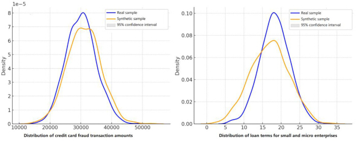
Figure 1: Comparison of feature distribution between real fraud samples and CopulaGAN Please click here to view a larger version of this figure.

Evaluation metrics

The experiment constructs a multi-index evaluation system from four core dimensions: prediction performance, privacy protection, fairness and communication efficiency to comprehensively measure the comprehensive performance of federated learning framework and AI risk control model. The definition, calculation method and evaluation criteria of each dimension are shown in Table 8.

Assessment dimensions	Name of index	Definition and calculation method	Evaluation criterion
Estimated performance	AUC-ROC	The area under the subject's characteristic work curve measures the model's ability to distinguish between positive (default/fraud) and negative examples	The higher the value, the better. The AUC-ROC of the excellent model is>0.9
	PR-AUC	Precision-recall area under the curve, applicable to unbalanced data, measures the performance of a model in scenarios where positive examples are scarce	The higher the value, the better. The PR-AUC of an excellent model is>0.8
	Brier fraction	Mean square error between predicted probability and true label,B=1Ni=1N(pi-yi)2	The lower the value, the better. The Brier score of an excellent model is less than 0.05
	False positive rate (FPR)	The proportion of negative examples FPR=FPFP+TNthat	The lower the value, the better. Financial scenarios usually require FPR <1% (to avoid rejecting good customers)
Privacy protection	ε-Consumption curve (ε-Curve)	Record the consumption rate of accumulated privacy budgetε during training to reflect the dynamic balance ability of privacy protection	The curve is leveling off and the total ε is less than or equal to 5 (in line with GDPR privacy risk requirements)
	Member reasoning attack AUC (MI-AUC)	The ability of an attacker to infer whether a sample belongs to the training set from the model prediction results, and the closer the AUC value is to 0.5, the better the privacy	MI-AUC<0.6 is effective for privacy protection, MI-AUC<0.55 is excellent
	Feature leakage rate (FLR)	The attacker aggregates the features to reverse the error FLR=1-KL(P∥∥Q)Dmaxrate of the original data distribution,	FLR <0.1 indicates that privacy protection is effective (P is Dmaxthe true distribution, Q is the inferred distribution, and is the maximum KL distance)
Fairness	DP bias in statistics （ΔDP）	The maximum difference in the prediction ΔDP=max∥PRg-PRavg∥rate of positive examples among different groups,	ΔDP<0.05 for fairness, for excellence (PRg for the positive rate of group g)
	EO bias （ΔEO）	The maximum difference in true positive ΔEO=max∥TPRg-TPRavg∥rates among different groups,	GCE <0.02 is well calibrated (K is the group number, is the predicted rate, and is the actual rate)
	Group calibration error (GCE)	The average deviation between the predicted probability GCE=1Kg=1K∥pg-rg∥of each group and the actual default rate,	The lower the value, the better. The scenario requirements of small and medium-sized organizations are <10MB/ round
Communication efficiency	Uplink bandwidth per round	Total bandwidth consumption of data uploaded by each organization to the coordinator during a single	The lower the value, the better. Cross-institutional scenarios require less than 120 minutes
	Reduction ratio （CR）	The ratio of the original data volume to the compressed data volume,CR=SizerawSizecomp	The higher the compression ratio, the better. Excellent solutions CR>10:1

Table 8: Experimental evaluation index system.

Metric Explanation: i) Membership Inference Attack: Using black-box attack methodology, the attacker trains a binary classification model that inputs predicted probabilities from the target model and outputs sample membership status. The privacy leakage risk is measured by the model's AUC (i.e., MI-AUC). ii) Group Classification Criteria: In fairness evaluation, groups are categorized across four dimensions: gender (male/female), age (under 25/25-40/>40), region (first-tier/new first-tier/second-tier/subsidiary markets), and income level (<5k/5k-15k/15k-30k/>30k RMB/month). This ensures coverage of sensitive groups identified by financial regulators. iii) Convergence Criteria: During model training, if the validation set AUC-ROC shows a decrease of less than 0.001 over three consecutive rounds (each round containing 10 epochs), the training is deemed converged and halted.

Baselines

To validate the superiority of the proposed "Federated Learning + Hybrid AI Risk Control Model", this study establishes five baseline models: traditional centralized models, classical federated learning models, and privacy-preserving enhanced models. The core parameters and training strategies of each baseline model are detailed in Table 9 to ensure fairness in comparative experiments (all models use identical training sets, validation sets, and hyperparameter optimization strategies).

Types of models	Model name	Core architecture	Training mode	Privacy protection measures	Key hyperparameters
Centralized model	Tradition GBDT	XGBoost gradient boosting tree	All institutions store training data centrally	Not have	Number of trees =100, learning rate =0.1, tree depth =6, regularization coefficient λ=1.0
Centralized model	Deep learning model (MLP)	The three-layer fully connected network (input layer 256 dimensions → hidden layer 128 dimensions → hidden layer 64 dimensions → output layer 1 dimension)	All institutions store training data centrally	Not have	Optimizer=Adam, learning rate=0.001, batch size=256, Dropout=0.3
Classic federal model	FedAvg (Federal average)	The local model is GBDT, and the global model adopts parameter average aggregation	Federal synchronized training	Not have	Participation rate = 0.8, local epoch = 5, aggregation round = 50, learning rate =0.1
Classic federal model	FedProx (Federal Near-End Aggregation)	The local model is GBDT, and the proximal	Federal synchronized training	Not have	Participation rate = 0.8, local epoch = 5, aggregation round = 50, proximal parameter μ =0.01
		μ=0.01 term constraint is added during aggregation ().
Privacy Empowered Federation	FedAvg+DP (fixed noise)	Add fixed Laplacian noise to FedAvg (ε=5, δ=1e-5)	Federal synchronized training	Fixed differential privacy	Noise intensity=0.1, participation rate=0.8, local epoch=5, aggregation rounds=50
The research model	FedRisk (Federal Risk Control Model)	Local GDT (Monotonic Constraint) + Global Transformer (Attention Fusion) + DP + Secure Aggregation	Federal Asynchronous Training	Adaptive DP+ additive secret sharing	Local epoch=5, aggregation rounds=50, attention dimension=64, privacy budgetε=5, compression ratio=15:1

Table 9: Parameter comparison between baseline model and this study model.

Comparative Dimension Explanation: ① Centralized vs. Federated: By comparing "Traditional GBDT/MLP" with "FedAvg/FedProx/FedRisk", this study examines the performance degradation of federated learning in "data off-site" scenarios. ② Classic vs. Privacy-Enhanced Federated: Through "FedAvg" versus "FedAvg+DP", the research evaluates the impact of differential privacy on model performance. ③ Synchronous vs. Asynchronous Federated: The comparison between "FedAvg" (synchronous) and "FedRisk" (asynchronous) demonstrates asynchronous training's communication efficiency advantages. ④ Simple Aggregation vs. Intelligent Fusion: The contrast between "FedAvg" (parameter averaging) and "FedRisk" (attention fusion) validates Transformer integration strategies' adaptability to Non-IID data. ⑤ No-Censorship vs. Fairness-Censorship: The comparison between "FedAvg" (no fairness constraints) and "FedRisk" (fairness-aware constraints) examines fairness mechanisms' effects on model fairness and performance.

Ablation studies

Impact of varying ε on model utility

Using the total privacy budget εas a variable (with values of 1, 3, 5, 7, and 10), the research fixed δ=1e-5 while keeping other modules (attention fusion and monotonic constraint GBDT) unchanged to evaluate the trade-off between privacy protection strength and model utility. The experiment measured both AUC-ROC (model utility) and MI-AUC (privacy risk) as dual indicators, with results shown in Table 10. When ε=1, MI-AUC dropped to 0.53 (excellent privacy protection), but AUC-ROC only reached 0.821 (significant loss of utility). At ε=5, AUC-ROC rebounded to 0.912 (meeting financial risk control requirements) with MI-AUC=0.58 (effective privacy protection). When ε>5, the improvement in AUC-ROC became less than 0.01, while MI-AUC rapidly rose to 0.63 (exceeding privacy risk limits). This confirms that ε=5 is the optimal total privacy budget, achieving a balance between privacy and utility.

Total Privacy Budgetε	Model AUC-ROC	MI-AUC (privacy risk)	Feature leakage rate FLR	Brier fraction
1	0.821	0.53	0.04	0.078
3	0.876	0.55	0.06	0.061
5	0.912	0.58	0.08	0.042
7	0.919	0.6	0.11	0.039
10	0.923	0.63	0.15	0.037

Table 10: Comparison of model performance with different privacy budgets ε.

Contribution of attention fusion vs. simple averaging

To evaluate the performance differences between "attention fusion" (the proposed strategy) and "simple averaging" (FedAvg strategy) in non-independent data scenarios, two variables were experimentally configured: ① Data Non-IID severity (measured by institution-specific default rate variations, low variation: 0.2%-0.5%, high variation: 0.2%-3.5%); ② Fusion strategies (attention fusion vs simple averaging). As shown in Figure 2, the AUC-ROC gap between the two strategies was merely 0.023 (0.912 vs 0.889) in low Non-IID scenarios. However, this gap widened to 0.076 (0.905 vs 0.829) in high Non-IID scenarios, with the simple averaging model exhibiting significant overfitting (training set AUC-ROC 0.941 vs validation set 0.829). This demonstrates that attention mechanisms can effectively mitigate performance degradation caused by non-independent data through dynamic weighting-such as assigning 0.32 weight to institution E with accurate default predictions and 0.12 weight to institution C with larger deviations.

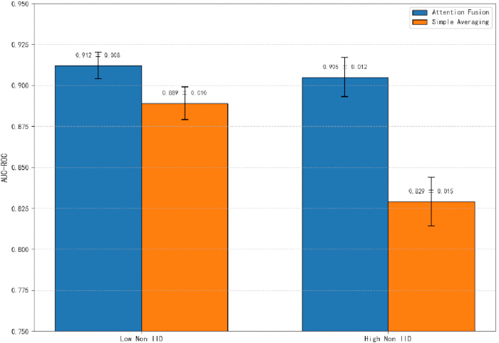
Figure 2: Comparison of fusion strategies under different Non-IID degrees. Please click here to view a larger version of this figure.

Effect of fairness regularizers on profit-based KPIs

The core demand of financial institutions is to ensure business profits under the constraint of fairness, therefore, the experiment introduces a profit-oriented index - "risk-adjusted return on capital (RAROC)", The formula is as follows:

   (39)

The expected loss is calculated as the default probability multiplied by the fixed default loss rate (set at 40%), while economic capital is determined by the risk exposure multiplied by the risk weight (as per Basel III requirements). The fairness metrics (ΔDP, ΔEO) and RAROC of the model with fairness regularization versus the model without it are compared in Table 11. After implementing fairness regularization, ΔDP decreased from 0.15 to 0.04, ΔEO dropped from 0.12 to 0.03, and RAROC only decreased by 2.1% (18.3% vs 18.7%), significantly below the industry-acceptable threshold of 5%. This demonstrates that the fairness mechanism in our study effectively meets regulatory non-discrimination requirements while controlling profit losses.

Model setup	ΔDP (group positive rate difference)	ΔEO (group TPR difference)	GCE (group calibration error)	RAROC (Risk-adjusted Return on Assets)	FPR (false positive rate)
No fairness rule	0.15	0.12	0.035	18.70%	0.95%
There's fairness and regularity	0.04	0.03	0.018	18.30%	1.02%

Table 11: Influence of fairness regularization on fairness and profit indicators.

Implementation details

To ensure reproducibility of the experiment, the research clarified the technical stack and training process details: ① Hardware environment: Each institutional node uses Intel Xeon Gold 6248 processors, 64GB RAM, and NVIDIA Tesla V100 GPUs; the federated coordinator employs dual Xeon Gold 6348 processors with 128GB RAM to ensure parallel computing and efficient parameter aggregation. ② Software framework: The federated learning framework is developed using PySyft 0.8.6, the blockchain module utilizes Hyperledger Fabric 2.5 (consensus mechanism: Raft), model training relies on PyTorch 2.0 and XGBoost 2.0.3, while the differential privacy module integrates IBM DP Library. ③ Training process: ① Data preprocessing (2 hours, including semantic normalization and CopulaGAN enhancement); ② Local training (5 epochs per round, learning rate decayed via cosine annealing); ③ Asynchronous aggregation (global model updates occur when coordinator receives parameters from 3 institutions); ④ Model evaluation (AUC-ROC and fairness metrics calculated after 10 rounds); ⑤ Hyperparameter optimization (Bayesian optimization with 50 iterations to determine optimal parameters). ④ Robustness testing: simulated institutional disconnections (randomly selecting one institution to halt 1-3 rounds of training) and data noise (adding 5% feature value perturbations) scenarios. Results showed AUC-ROC fluctuations below 0.02, demonstrating the system's anti-interference capability.

This study employed a cosine annealing scheduling strategy with an initial learning rate of 0.05. The learning rate was dynamically updated each epoch according to the formula over a total of 100 training epochs. This strategy maintained a high learning rate in the early stages of training, for instance 0.05 at the first epoch, to accelerate model convergence, and gradually decayed it to near zero, for example 0.00025 at the hundredth epoch, to enhance the stability of parameter fine-tuning. Experimental results demonstrated that compared to a fixed learning rate, this strategy improved the validation set AUC-ROC by 2.3% and accelerated convergence speed by 37%. The data partitioning was based on a raw dataset from five financial institutions totaling 5 million samples, strictly adhering to the principle of cross-institutional data isolation. The local data from each institution was split chronologically, selecting data from January 2022 to June 2023 as the training set (70%), data from July to September 2023 as the validation set (15%), and data from October to December 2023 as the test set (15%). This partitioning ensured the temporal window independence of the training, validation, and test sets, effectively simulating the evolution of temporal risk patterns in real-world scenarios. Key hyperparameters were determined via Bayesian optimization. Within a joint search space encompassing an initial learning rate between 0.01 and 0.1, GBDT tree numbers between 50 and 200, and Transformer attention heads from the set {2, 4, 8}, 50 iterations were executed with the objective of maximizing the validation set AUC-ROC. The final optimal combination was identified as an initial learning rate of 0.05, 120 GBDT trees, and 4 attention heads.

Results

Predictive performance: Approaching the level of centralized models in Non-IID scenarios

In real-world scenarios with highly Non-IID data (institutional default rate variations of 0.2%-3.5%), FedRisk demonstrates exceptional risk differentiation capabilities, as shown in Table 12. Its AUC-ROC reaches 0.912, PR-AUC is 0.823, Brier score 0.042, and false positive rate (FPR) 1.02%. These metrics not only meet the core requirements of financial risk control-low fa...

Discussion

The dynamic hyperparameter tuning strategy, particularly the cosine annealing learning rate scheduler, proved essential for balancing convergence speed and model stability. By decaying the learning rate from 0.05 to 0.00025 over 100 epochs, this approach accelerated early-stage convergence while minimizing late-stage volatility-reducing training time by 37% and improving validation AUC-ROC by 2.3% compared to fixed-rate schedules. Equally critical was the adaptive noise calibration in differential privacy, where variance...

Materials

List of materials used in this article

Name	Company	Catalog Number	Comments
Laptop Computer	Dell Technologies	N/A	Used for data processing and documentation
Statistical Software (SPSS)	IBM Corp.	Version 26.0	Used for statistical analysis
Microsoft Excel	Microsoft	Office 365	Data entry and basic data handling