Analyzing the Environmental Footprint and Its Determinants in China: An Integrated Assessment of the EKC and Pollution Haven Hypotheses

Summary

This research confirms that energy use and open trade degrade the environment, supporting the pollution haven hypothesis. It advises policymakers to pursue sustainable tourism, diversify energy sources, and attract foreign investment into service sectors for better ecological outcomes.

Abstract

This study provides a comprehensive empirical investigation into the determinants of China's environmental footprint from 1990 to 2023, with a specific focus on testing the Pollution Haven Hypothesis (PHH) and the Environmental Kuznets Curve (EKC) in the context of travel and tourism. Employing the EKC framework, we analyze the dynamic impacts of eco-tourism, economic growth, energy consumption, trade openness, and foreign direct investment on ecological degradation. The methodology involves advanced statistical tests to establish the existence of a long-run equilibrium relationship among the variables. The findings confirm an inverted U-shaped EKC relationship between travel and tourism development and the environmental footprint, indicating that the sector initially exacerbates environmental degradation but, beyond a certain threshold of economic development, contributes to its amelioration. Further results indicate that energy utilization and trade openness significantly intensify the environmental footprint. Crucially, foreign direct investment is found to escalate environmental degradation, thereby providing robust empirical support for the Pollution Haven Hypothesis in the Chinese context. Consequently, this study recommends that policymakers prioritize the transition towards sustainable tourism models, accelerate the diversification of the energy mix towards cleaner sources, and strategically channel foreign direct investment into less polluting service sectors.

Introduction

Global climatic changes resulting from human actions are making a low-carbon economy an unavoidable necessity for the local authorities of the global edge¹. Unusual weather occurrences can disrupt stream flow, the dynamics of the organisms within an ecosystem, instabilities in agricultural production², damage associated with infrastructure, or increased morbidity and mortality, thereby indicating that the socio-economic, biological and geographical processes have induced variability and forced scholars to proceed to the driving of this change³. Ecotourism is associated with ecological costs because of the increase in ecotourists through its related pollutants⁴. Since it generates profits, builds infrastructure, creates employment opportunities and earns valuable foreign currency, the travel and tourism industry is a trillion-dollar business⁵, and it is 7.6% of the world today⁶_, when the United Nations World Tourism Organization (UNWTO) reported that travel and tourism was responsible for 1 in ten jobs worldwide, 7% of global trade, and 10 percent of the world's GDP⁷. The increase in the number of visitors was one of the drivers of pollution-related emissions and material waste generation⁸.

Prior research has established the tourism-environment link but often relies on broad econometric models that lack sector-specific operational guidance⁹. This article demonstrates a structured analytical protocol integrating Energy Input-Output Analysis and Carbon Footprint Assessment to map direct and indirect energy flows and emissions across tourism sub-sectors. Unlike existing techniques, this method provides a granular, actionable breakdown for policymakers, moving from identification to targeted mitigation¹⁰. Climate impacts necessitate a low-carbon transition in tourism, a major global economic sector¹¹. However, existing research lacks nuanced empirical analysis for major polluting economies with unique developmental pathways^12,13. China presents a critical case study: it is the world's largest carbon emitter, possesses a tourism sector undergoing rapid expansion, and has an energy mix dominated by fossil fuels, creating a distinct tension between growth and sustainability. This study addresses a significant gap by investigating the non-linear Environmental Kuznets Curve relationship between tourism development and environmental footprint in China, while concurrently testing the pollution haven hypothesis through foreign investment flows. Our contributions are threefold: (1) providing China-specific, policy-relevant evidence on tourism's environmental trajectory, (2) integrating an analysis of energy structure and investment policy into the tourism-environment nexus, and (3) offering a methodological framework that distinguishes between short-run pressures and long-run sustainable pathways, thereby advancing the empirical literature beyond generalized cross-national findings.

This vision, described as a "True North a "planet initiative" to secure affluence and save the environment¹⁴, is operationalized through frameworks like the United Nations' Sustainable Development Goals (SDGs) or "The 2030 Agenda," which comprises 17 goals and 169 targets¹⁵. Within this, sustainable tourism, promoted by the UN's declaration of 2017 as the International Year of Sustainable Tourism for Development¹⁶, is guided by principles such as those from the UNWTO emphasizing sustainable economic growth, inclusivity, and environmental protection¹⁷. Eco-tourism, which operates on the three pillars of social, economic, and environmental sustainability¹⁸, offers commercial, cultural, and environmental benefits¹⁹, by reconciling communities, climate, and the travel industry and enhancing resource reliability. Some nations already utilize tourism revenues for conservation, and it is recommended that all countries institute strategies to attract environmentally conscious tourists and enforce industry laws that protect the climate and resources²⁰.

The protocol is designed for national or regional-scale application and assumes the availability of reliable tourism expenditure data and integrated energy-economic tables. A key limitation is its dependency on the resolution of this input data. Under these conditions, it enables authorities to pinpoint high-impact activities, assess renewable energy integration potentials, and design evidence-based regulations to transition towards a low-carbon tourism economy, thereby supporting ecological and economic sustainability^21,22.

The environmental impacts of tourism are multifaceted, manifesting as heightened carbon emissions, waste, and resource depletion from vehicular and infrastructural demands, which collectively drain climatic and mineral wealth²³. This is evidenced by the increased energy consumption and resultant CO₂ emissions driven by growing visitor numbers, a global phenomenon that has prompted governmental shifts towards establishing low-carbon business models²⁴. Empirical evidence suggests a willingness among certain demographics, such as middle-aged males and ecotourists, to pay a premium for renewable energy use in accommodations, acknowledging its environmental benefit²⁵. Furthermore, tourism intensifies pressure on vital resources, escalating the demand for water and sanitation facilities and challenging their wise management²⁶. Scholarly investigations confirm this link, revealing that the top forty-eight ecotourism nations, with the exception of some European countries, face increased CO₂ emissions from tourism²⁷, a correlation also established in OECD countries and specific Chinese provinces²⁸. Research in 16 Mediterranean countries identified a combined effect of agriculture and tourism on green resources and established bidirectional causal relationships among renewable energy, GDP, and tourism, with one study confirming a 0.14% increase in tourism revenue for every 1% rise in CO₂ in the region²⁹. Conversely, in France a top global destination tourism and population growth have been linked to contamination reduction, while other studies highlight complex, bidirectional connections between financial development, electricity usage, and tourism in leading ecotourism areas³⁰. The scale of the issue is significant, with the global carbon footprint of tourism calculated to have risen from 3.9 GtCO₂e in 2009 to 4.5 GtCO₂e in 2013 across 160 nations, though the effect varies by region, exhibiting positive, negative, and null impacts on the climate in Tunisia, Egypt, and Morocco, respectively³¹.

Research examining the tourism-environment nexus reveals complex and region-specific dynamics, found the climatic impact of tourism to be positive in Tunisia, negative in Egypt, and neutral in Morocco, with the relationship between income and CO₂ in the latter two nations confirming the Environmental Kuznets Curve (EKC) hypothesis³². This hypothesis was further supported in OECD economies, where CO₂,was found to be Granger-caused by both visitor numbers and the EKC relationship³³. Case studies from specific destinations highlight this duality; in Pattaya, Thailand, tourism yielded both positive ecological planning and negative waste and pollution effects, while in Turkey, studies confirmed that a 1% increase in real income raised CO₂ by 0.345%, with tourism and energy use identified as causal factors³⁴. At a broader scale, an analysis of BRICS nations showed a 0.5313% increase in CO₂ per 1% accretion in tourist receipts, though a feedback causality also suggested that a 1% rise in tourist financing could lead to a 0.5771% decrease in CO₂. Conversely, research in Central and South America asserted unidirectional causality from renewable energy to CO₂ reduction and found that environmental degradation abated due to tourism, FDI, and renewables³⁵, a finding complemented by the confirmation of an inverted U-shaped EKC between economic globalization and carbon impact in South Asia. Finally, quantifying this impact, the annual carbon emissions from tourism in Barcelona were estimated at 9.6 MtCO2 eq., equating to 96.9 kg CO₂ eq. per visitor daily³⁶.

This study distinguishes itself within the extensive literature on tourism's impact on CO₂, emissions by constructing a unique global tourism metric comprised of (i) domestic travel and tourism consumption, (ii) government personal travel expenditures, (iii) public investment, (iv) international tourist receipts, and (v) foreign visitor spending, expressed in terms of total environmental impact. Rather than a singular grouping, the analysis categorizes countries by income level to investigate the impact of tourism, economic growth, and renewable resources, alongside the relationships between these variables. This approach contributes to a nuanced understanding, particularly as the existing body of research presents conflicting conclusions. For instance, while eco-tourism branding as a key policy tool for conservation³⁷, and the expansion of the carbon footprint from major tourist-originating nations, findings on the Environmental Kuznets Curve (EKC) are mixed. Some studies affirm that tourism can trigger the EKC, suggesting it may foster environmental durability in high-income economies, despite tourist arrivals and receipts generally having a harmful effect on emissions³⁸. Conversely, other research rejects the Kuznets postulate in high-income states or finds an increasing monotonic relationship between tourism revenue and environmental cost³⁹.

Protocol

Theoretical framework and variable selection
The empirical model and variable selection for this study are explicitly derived from a synthesis of foundational theories that explain the dynamic relationship between economic development and environmental sustainability. The investigation is principally guided by the Environmental Kuznets Curve (EKC) hypothesis⁴⁰, which posits an inverted U-shaped trajectory where environmental degradation initially increases with economic growth but eventually declines after a certain income threshold is reached. To test this core proposition, Gross Domestic Product (GDP) is included as the primary indicator of economic scale and development. Concurrently, the analysis integrates the tourism-led growth hypothesis, necessitating the inclusion of Tourism and Travel (T&T) as a percentage of GDP to assess the sector's dual role as both an engine for economic expansion and a potential source of increased resource consumption and pollution. The theoretical expectation of a non-linear relationship leads to the incorporation of a squared T&T term within the model to empirically capture the potential EKC turning point specific to the tourism sector. Further theoretical grounding is provided by the pollution haven hypothesis, which suggests that stringent environmental regulations in developed economies can lead to the relocation of polluting industries to countries with laxer standards. To empirically evaluate this claim for China, Joint Venture (JV) inflows are incorporated as a proxy for foreign direct investment, testing whether such capital flows exacerbate the domestic environmental footprint. The model also acknowledges the critical role of energy systems through the lens of the IPAT (Impact = Population × Affluence × Technology) framework, which identifies energy consumption as a fundamental proximate driver of ecological impact. Consequently, Energy Use (EU) is included as a key independent variable, reflecting the pollution intensity inherent in a nation's energy mix. Finally, the model accounts for Open Trade (OT), informed by trade theory, which postulates that international commerce influences the environment through scale (increased output), composition (shifts in industrial structure), and technique (technology transfer) effects. The selection of the comprehensive Environmental Footprint (EF) as the dependent variable is itself a theoretical choice aligned with ecological economics, as it provides a holistic metric of anthropogenic demand on bioproductive ecosystems, effectively capturing the multidimensional environmental cost of economic activities^41,42. This coherent theoretical triangulation directly informs the construction of the sampled dataset, ensuring each variable represents a specific, theory-driven channel through which China's socioeconomic evolution impacts its ecological base.

Data and model specification
From 1990 to 2023, this research used yearly basis series records from China. The study's dependent variable, which can replace environmental pollution, is an environmental footprint. In other words, the EF provides the number of hectares of territory and the river needed to sustain territory usage. According to one theory, environmental costs with higher values show greater environmental harm. The entire ecosystem is employed to gauge environmental damage. Tourism revenues, touristic spendings, and the percentage of visitors have largely taken the position of tourist industry advancement factors in relevant literature⁴³. Carbon impact is the report's reliant factor. This study was a pioneer in using data on tourism and travel as a percentage of GDP to look into how it affected China's environmental footprint. Following the work of Mrabet and Alsamara⁴⁴, energy consumption was also included in the study. Data were gathered for the present research from the World Development Indicators. China statistical yearbook and the China Bureau of Statistics both provided information on the growth of tourism in China. Additionally, information on the footprint was obtained from the Global Footprint Network (2018)⁴⁵, and the World Data Atlas provided information on the travel and tourist industry as a share of GDP.

Analytical framework
According to the latest research, the growth of the touristic industry significantly raises the amount of environmental effects. As a result, we define the next econometric estimable equation, which comes after^46,47 as follows:

       (1)

GDP stands for economic development, where EF is a stand-in for environmental footprint and EU for energy utilization. For the purpose of examining its effects on China's environmental cost, this research involved traveling as well as the tourist industry as a percentage of GDP (T&T). Additionally, the sum of squares term for visitor numbers and travelling is added to test the Kuznets curve-type connection between carbon impact and the tourist industry. The system represents foreign direct investment (FDI) to examine whether its inflows play a significant role in determining environmental integrity by following the Carbon emissions Sanctuary Speculation or Contamination Halo Speculation⁴⁸, Additionally, trading liberalisation, that is also a crucial possible factor of environmental protection, was highlighted in this report's environmental arena in accordance with the work of⁴⁹. The following is the econometric model.

      (2)

The latest research used the natural graph of the report's factors to get the immediate elasticities of co-efficient and to simplify the estimation procedure. Thus, the following is a modification of the equation;

      (3)

Estimation approach
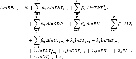
The current research initially examines the information's smoothness to determine whether it is level or stationary. An appropriate cointegration analysis that can be used in this situation is the auto regressive lag (ARDL). It is debated that the ARDL bound assessment method is better to different methods based on its qualities, which include the following: it can be utilized despite of sequence of correlation of factors, either they are I(0) or I(1) or a blend, this can concurrently evaluate shorter and prolonged results; it encompasses the issue of exogenous variables and remainder connection because of the correct lags selection, it has decent limited test qualities as comparison to Johansen approach⁵⁰. The method of records generation encapsulates sufficient lags when switching from such a common outline to a particular structure for accurate guesstimates⁵¹. Additionally, using a straightforward linear transformation, we can integrate short-term adjustments to create a mechanism for error correction without upsetting the long-term balance. The research concentrates on error-correcting mechanisms under ARDL for short-run estimates and Ordinary Least Squared (OLS) based measures for the prolonged period. The current study employed a double log framework, suitable with for Malaysia⁵², and took factors in log form to avoid auto-correlation and multi-collinearity concerns. The ARDL technique was used in this research to identify the following long-run presence connections:

      (4)

Where the standard error is shown by β₀ is the constant term. The upcoming portion of computation, symbolized by λ denotes prolonged connections, while the summing up icons depict dynamics in the short run. To determine as to if variables are included in the long-run or not, the research chose a bound test. It is claimed that the approximated F-statistics value surpasses the maximum bound at which cointegration can be predicted to exist. The cointegration test was further evaluated in the present study. Numerous investigators have created various cointegration techniques in the econometric literary works, with varying outcomes and features. A consolidated test was created to improve the capacity of correlation based on a number of prior cointegration methods. For even more comprehensive estimation methods, this technique offers combined statistics to test zero points devoid of cointegration. Cointegration will be accepted if the null hypothesis is rejected. According to the sum of the measured levels of significance (p-values) for each cointegration test under Fisher's formula is as follows:

      (5)

      (6)

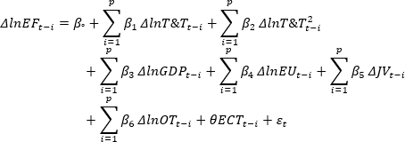
In this, EG stands for Engle and Granger statistics, and JOH stands for Johansen test statistics⁵³. It is demonstrated that BDM, and BO presents the Boswijk test statistics⁵⁴. Similar to how the regarded acronyms for these assessments show the p-values of cointegration, we would dismiss the no-cointegration hypothesis if the tabulated values are below the guesstimated Fisher' statistics. Additionally, the following short-run assessments would be made by using the correction of errors mechanism:

    (7)

Results

Preliminary Analysis
A thorough preliminary analysis of the data is a fundamental prerequisite for robust econometric modeling, as it establishes the essential characteristics and behavior of the underlying variables. This stage involves examining descriptive statistics to understand central tendencies, dispersion, and normality, while graphical inspections such as box plots and growth rate trends provide critical visual insights into the distribution, variability, and temporal evolution of the series. This foundational step is crucial for identifying potential outliers, understanding the scale of variables, and forming initial hypotheses about relationships, thereby informing the appropriate selection of subsequent econometric techniques and guarding against spurious results derived from misunderstood data properties.

Table 1 descriptive analysis and correlation are examined in this research. According to Jarque-Bera statistics, to environmental impact, increase in the travel sector, electricity use, economic expansion, trade openness, and direct foreign investment are all divided evenly. The findings demonstrate that the carbon impact has a mean value of 11.82, a range of 11.34 to 12.21, and no significant variations. GDP and JV are the variables that vary the most, with an average figure of 4.13 and 1.21, a minimal figure of 1.01 and 0.37, and the highest values of 7.54 and 3.67, respectively. However, there aren't any more significant variations in the growth of the tourist industry, commerce, or energy utilization during the period of investigation. Last but not least, over the observation time frame, commerce and power utilization do not exhibit those kinds of differences from mean values.

Table 2 offers a focused perspective of the growth rates of the annual percentage change of key variables, including Environmental Footprint (EF), Tourism & Travel (T&T), Gross Domestic Product (GDP), Energy Usage (EU), Carbon Impact, Visitor Percentage, and Tourism Revenue every four years. It presents a snapshot of the patterns of the trends in these variables across four-year differences. In so doing, it reveals the way in which the rates were changing across different periods. The fluctuating rates, from positive to negative and back again reflect the dynamic nature of China's environmental, economic, and tourism sectors and the way in which the direction of the country's trajectory changed over time. As this periodic perspective reveals, the changes of growth and decline occurred at regular intervals, punctuating the overall rates and identifying moments of growth or decline that were taking place throughout this study's timeframe.

Figure 1 shows vertical box plots display the median, quartiles, and variability of Environmental Footprint (EF), GDP, Tourism & Travel (T&T), and Energy Use (EU) in China over the sample period.

Figure 2 shows the horizontal box plots that visualize the spread, central tendency, and potential outliers for Environmental Footprint (EF), GDP, Tourism & Travel (T&T), and Energy Use (EU) in China across the study period.

Econometric methodology and pre-testing
The validity of any time-series analysis hinges on rigorous pre-testing to ensure the data meets the necessary statistical assumptions, thereby preventing misleading inferences. This phase involves conducting unit root tests, such as the Zivot and Andrews test, to determine the stationarity properties of the variables and account for potential structural breaks a vital step to avoid the pitfalls of spurious regression. Following this, cointegration testing via the ARDL bounds approach and complementary methods is employed to ascertain the existence of a stable long-run equilibrium relationship among the variables, which is a mandatory condition for estimating meaningful long-run coefficients. These diagnostic procedures collectively validate the chosen Autoregressive Distributed Lag (ARDL) framework as the appropriate and robust methodology for investigating the dynamic interplay between tourism, economic growth, and environmental footprint in China.

Table 3 reveals the diverse metrics across six Chinese regions. North China has a moderately low EF (15.49) but an enormous energy usage (1667.24) and GDP (6976.31). South China possesses the maximum EF (17.15), while also leading tourism & travel (9.13), and GDP (9479.18), indicating a degree of correlation between economic activity and environmental impact. East China and West China both found themselves with metaphorical middle-ground EFs (16.03 and 15.45, respectively), but diverged notably in GDP and energy usage, East China with a lower GDP (3497.25) but higher energy usage (1967.93). Central China was in possession of the lowest EF (14.24), but also in possession of the lowest GDP (3141.53), a differing economic-environmental dynamic. Northeast China's EF (16.46) is sandwiched between moderate to high values across all categories, with Tourism & Travel (7.3), and GDP (8828.34) being noteworthy examples. The numerical variation within these categories speaks to the uniqueness of environmental and economic profiles, and in turn the complexity of regional development and environmental impact, in China

Table 4 presents the results of the Zivot and Andrews unit root test, which assesses the stationarity of the variables while accounting for a single endogenously determined structural break. The findings indicate that at levels, the variables for Tourism & Tourism-squared (T&T, T&T2), Open Trade (OT), and Joint Ventures (JV) are stationary, as their t-statistics are significant at the 5% level, with structural breaks identified between 2003 and 2007. However, the Environmental Footprint (EF), GDP, and Energy Use (EU) series are non-stationary at levels. When these variables are transformed into first differences, EF, EU, and JV become stationary, confirming they are integrated of order one, I(1). This mixed order of integration justifies the use of a cointegration approach that is robust to structural breaks for subsequent analysis.

Figure 3 shows the four-panel time series plot illustrates the historical trajectories of Environmental Footprint (EF), GDP, Tourism & Travel (T&T), and Energy Use (EU), highlighting their co-movement and growth patterns over three decades.

Table 5 presents the outcomes of the bounds testing procedure for cointegration within an ARDL framework. The results confirm the existence of a significant long-run cointegrating relationship in all seven models where a different variable is specified as the dependent variable. This is evidenced by the computed F-statistics for each model, which exceed the upper-bound critical value at the 1%, 5%, or 10% significance levels. The selected ARDL lag structures, which vary across models, indicate different short-run dynamic adjustments among the variables. These robust findings validate the presence of a stable long-run equilibrium relationship between the environmental footprint (EF), travel and tourism (T&T), economic growth (GDP), energy use (EU), open trade (OT), and joint ventures (JV), forming a solid foundation for estimating long-run coefficients.

Table 6 discusses all the descriptive statistics and various tests. The Engle-Granger Johansen (EG-JO) test results in a T-statistic of 20.297 which exceeds the 5% critical value of 10.420, indicating there is cointegration among the variables. As well, using the Boswijk-Ben and Banerjee (BO-BDM) test along with the EG-JO produces a T-statistic of 21.002 which is above the 5% critical value of 19.888, which again indicates cointegration with the variables. These results imply that the variables in question are highly related and potentially in long-run equilibrium.

Figure 4 shows scatter plots illustrating the relationships between Environmental Footprint (EF) and Gross Domestic Product (GDP), and between Tourism & Travel (T&T) and Energy Usage (EU). Each plot includes a fitted regression line to highlight overall trends. The EF GDP plot suggests a slight positive association, while the T&T EU plot shows a weak, nearly flat relationship. These visuals help assess the strength and direction of correlations among the variables.

Long-run results of ARDL
The ARDL long-run results are presented in and they demonstrate that tourism and travel in China contribute to environmental deterioration as their GDP contributions rise along with the nation's environmental cost. According to the results, a rise in tourism and travel spending of 1% would result in an almost 2.3% increment in CO₂ emission spending.

Table 7, the long-run analysis confirms a statistically significant inverted U-shaped relationship between travel and tourism (T&T) and the environmental footprint, thereby validating the Environmental Kuznets Curve (EKC) hypothesis for China. The positive coefficient for T&T and the negative coefficient for T&T² indicate that tourism initially increases environmental degradation, but after reaching a calculated turning point, it begins to reduce it. Furthermore, economic growth (GDP) and energy use (EU) significantly increase the environmental footprint, while open trade (OT) appears to reduce it. Joint ventures (JV) have a smaller but statistically significant positive impact, supporting the pollution haven hypothesis. The model is robust, with a good fit (R² = 0.67) and no issues of non-normality or heteroscedasticity.

Short-term outcomes of ARDL
According to Table 6's findings for the short term, traveling and tourism have a negligible effect on the nation's environmental footprint. On the contrary, travel and tourism as a whole could have a very positive effect on China's environmental footprint. This demonstrates that China's tourism industry is environmentally friendly, as evidenced by its resistance to local pollution growth. There is evidence that, even in the short term, increasing tourist industry operations and making them almost twice as large would then enhance the ecosystem and promote economic development that is self-sustaining. The report's outcomes are in line with some research and the pioneering literature that holds that tourist numbers have a viable connection to the environment.

In Table 8, the dynamic adjustments of the variables are captured alongside the crucial error correction mechanism. The highly significant and negative coefficient of the CointEq(-1) term (-0.927) confirms a rapid speed of adjustment back to long-run equilibrium following a short-run shock, with approximately 93% of any disequilibrium being corrected within one period. In the short run, the one-period lag of tourism-squared (D(T&T^2)(-1)) and economic growth (D(GDP)) exhibit a significant positive pressure on environmental degradation. Similarly, both current and lagged energy use (D(EU) and D(EU)(-1)) significantly increase the environmental footprint. Open trade (D(OT)) shows a significant short-run benefit by reducing the footprint, while joint ventures (D(JV)) significantly worsen it, providing immediate support for the pollution haven hypothesis.

Toda-Yamamoto causation test outcomes
To avoid biased estimates from potential mixed order of integration I(0) and I(1), this study employs the Toda-Yamamoto (T-Y) approach to Granger non-causality⁵⁵.The test is applied within a VAR model where the optimal lag length (*k*) is determined by information criteria (e.g., AIC), and the maximal order of integration (d_max) is added to ensure robustness. Causality is tested using a standard Wald test (χ² statistic) for the first *k* lags of the hypothesized causal variable. A p-value below the 0.05 significance threshold leads to the rejection of the null hypothesis of non-causality, confirming a statistically significant Granger-causal relationship. The T-Y results reveal a bidirectional causality between China's environmental footprint (EF) and energy use (EU), and between EF and tourism & travel (T&T). This indicates a feedback loop where changes in these variables significantly influence each other. A unidirectional causality runs from joint venture (JV) inflows to EF (p < 0.05), supporting the pollution haven hypothesis, but not vice-versa. In contrast, no significant short-run causality was found between open trade (OT) and EF at the 5% threshold, suggesting trade's environmental impact is channeled through longer-term equilibria. These findings clarify the immediate dynamic interactions that underpin the long-run cointegrating relationships established earlier.

Table 9 shows the counterfactual analysis of policy changes from 2005 to 2018, presented in Table 9, reveals distinct trade-offs between economic and environmental objectives. The impact estimates were generated by applying the calibrated Autoregressive Distributed Lag (ARDL) model to simulate a baseline "no-policy" scenario for each variable. The percentage impacts reflect the model-derived average annual difference between this simulated baseline and the actual observed data following each policy's implementation, isolating the effect of the policy shock. The results show that stringent environmental regulations, such as the Carbon Emission Regulation and Green Energy Transition (2018), were most effective in reducing the environmental footprint (EF) and energy use (EU), with EF reductions of 8% and 7% respectively. However, these policies were associated with slight short-term declines in GDP and tourism (T&T), highlighting a potential cost to economic growth. In contrast, growth-oriented policies like the Economic Stimulus Plan (2008) and Tourism Development Initiative (2010) successfully boosted GDP and visitor numbers but had modest or negative impacts on environmental indicators. Crucially, policies such as the Renewable Energy Incentive Program and the National Ecotourism Plan demonstrate a more synergistic outcome, stimulating economic and tourism growth while simultaneously reducing environmental pressures. This suggests a viable pathway for decoupling development from environmental degradation when policies are designed to align incentives across sectors.

In Table 10, a network of significant causal relationships between the variables is identified. Most notably, a strong bidirectional causality exists between the environmental footprint (EF) and travel & tourism (T&T), confirming their interdependent relationship. Furthermore, unidirectional causality runs from energy use (EU) and open trade (OT) to EF, identifying them as drivers of environmental degradation. The results also reveal a tourism-led growth dynamic, as T&T causes economic growth (GDP), but not vice versa. Finally, a bidirectional causal link is found between T&T and joint ventures (JV), and between T&T and OT, highlighting the interconnected nature of tourism, investment, and trade. The error correction term is insignificant across all models, indicating that the captured causalities are primarily short-run in nature.

Figure 5 shows a heat map illustrating the Toda Yamamoto causation test outcomes across key variables, including EF, GDP, T&T, EU, Carbon Impact, and Sector Percentage. Higher intensity values indicate a stronger causal influence from the row variable to the column variable. This visualization highlights asymmetries in causal relationships and helps identify which factors exert the greatest directional impact.

Figure 6 shows that CUSUM plot displaying the stability of model parameters over time, with the cumulative sum of recursive residuals shown against the 5% significance bounds. The CUSUM line remaining within the confidence limits indicates parameter stability and absence of structural breaks. This visual test helps assess the robustness and reliability of the estimated model.

Figure 7 shows the CUSUM of Squares plot, illustrating the cumulative sum of squared recursive residuals relative to the 5% significance bounds. The movement of the curve within the confidence limits suggests stability in the variance of the model parameters over time. This diagnostic test helps detect potential structural changes affecting model consistency.

Table 11 has a detailed projection on changes with both curves forecasted In the five years from 2021 to 2025. As these statistics suggest, it future dynamics of environmental variables, economic factors and criminal laws will all be affected in China. The Environmental Footprint (EF) is forecast to grow steadily at 2.22% and the Tourism & Travel (T&T) sector by 2.68%, indicators of a consistent trend toward increasingly greater negative environmental impacts in both industries. Gross Domestic Product (GDP ) is predicted to grow with a robust 4.90% a year Chinese GDP will continue on its upward course. Energy Usage (EU) is expected to grow at 4.49%, indicating a steady rise in energy consumption. More notably, the Carbon Impact displays greater variation in this element, ranging from 2.04% to 5.26%! What this points out is that the carbon emissions environmental impact is particularly uneven. Visitor Percentage, which reflects the fluctuation of tourism dynamics, also has variations in forecasted growth rates. This in fact ranges from a base figure of 1.69% right on up to 4.72%. This fluctuation might be due to changing trends in global and domestic tourism, affected by policy changes, economic conditions and environmental awareness. Tourism Revenue is another important indicator for the tourism industry, forecast to vary between 1.36% and 2.69%. The economic benefits earned from tourism activities will continue to shift.

DATA AVAILABILITY
The datasets used in this study were taken from publicly available sources. The annual time-series data for China (1990-2023) can be accessed and downloaded from the following repositories to ensure full transparency and replicability: Environmental Footprint (EF): Global Footprint Network Data Platform (https://data.footprintnetwork.org).  Tourism & Travel (% of GDP), GDP, Energy Use, Joint Venture (FDI), Open Trade: The World Bank's World Development Indicators (https://databank.worldbank.org/source/world-development-indicators).  And Supplementary Tourism Data: National Bureau of Statistics of China (http://www.stats.gov.cn/english/).   

Figure 1: Vertical Box Plots Illustrating the Distribution of EF, GDP, T&T, and EU in China (1990-2020). Please click here to view a larger version of this figure.

Figure 2: Horizontal box plots depicting the variability of EF, GDP, T&T, and EU in China (1990-2020). Please click here to view a larger version of this figure.

Figure 3: Time Series Analysis of Environmental Footprint, GDP, Tourism & Travel, and Energy Usage in China (1990-2020). Please click here to view a larger version of this figure.

Figure 4: Scatter Plots with Regression Lines Examining Relationships Between EF, GDP, T&T, and EU. Please click here to view a larger version of this figure.

Figure 5: The heat map of Toda-Yamamoto causation outcomes. Please click here to view a larger version of this figure.

Figure 6: C.U.S.U.M plot. Please click here to view a larger version of this figure.

Figure 7: C.U.S.U.M. Squared. Please click here to view a larger version of this figure.

Table 1: Descriptive statistics Please click here to download this Table.

Table 2: Comprehensive Annual Growth Rates of Key Variables (1990-2020) Please click here to download this Table.

Table 3: Comparative Analysis Across Different Chinese Regions. Please click here to download this Table.

Table 4: Test Analysis of Zivot and Andrews Please click here to download this Table.

Table 5: Bounds testing outcomes Please click here to download this Table.

Table 6: Correlation outcome. Please click here to download this Table.

Table 7: Long-term variables. Please click here to download this Table.

Table 8: Short-run results. Please click here to download this Table.

Table 9: Policy Changes and Their Impacts on Key Variables. Please click here to download this Table.

Table 10: Toda Yamamoto causation outcomes. Please click here to download this Table.

Table 11: Forecasting of Future Trends for Key Variables (2021-2025). Please click here to download this Table.

Discussion

The findings of this study confirm the complex relationship between economic activities and environmental degradation in China, with critical implications for policy. Our application of the Toda-Yamamoto causality test and the ARDL cointegration method provided a robust framework for disentangling these dynamics. The success of this analytical protocol hinged on two critical steps: first, the establishment of a stable long-run cointegrating relationship among the variables, which validated the existence of a fundamental equilibrium link between tourism, energy use, foreign investment, and environmental footprint^56,57. Second, the use of the ARDL bounds testing approach was crucial for generating reliable short- and long-run estimates even with a mix of I(0) and I(1) variables, a common feature in macroeconomic time-series data⁵⁸. This methodological workflow directly led to the pivotal finding of an inverted U-shaped (EKC) relationship for tourism, as the model effectively captured the non-linear effect through the inclusion of a squared term, revealing that the sector's initial negative impact can transition to sustainability with further development and investment. Compared to simpler correlation analyses or standard regression that may miss dynamic equilibrium and causality, this integrated approach provides a more rigorous, temporally sensitive understanding of environmental drivers^59,60.

This protocol, while powerful, is not without constraints. Its primary limitation is its dependence on the quality and length of the national time-series data, which can obscure sub-national or sectoral heterogeneities. A common troubleshooting strategy for autocorrelation or heteroscedasticity issues often encountered in such models is to employ robust standard errors or incorporate appropriate lag structures, as was done here. Future applications could extend this method by disaggregating the "tourism" variable into specific components (transport vs. accommodation emissions) or by integrating it with spatial analysis to identify regional pollution havens within the country. Furthermore, the method's robustness for policy simulation is high, as it allows for testing the environmental impact of hypothetical changes in energy mix or investment policy. However, its usability for real-time decision-making is limited by data publication lags. When compared to Computable General Equilibrium (CGE) models, our approach is less data-intensive and more accessible for establishing historical causal inferences, though it lacks the detailed sectoral interplay forecast capability of a full CGE framework⁶¹.

Our study advances upon existing research by integrating the specific Chinese context of a fossil-fuel-dominated energy matrix and its status as a net exporter into a unified policy framework that directly confronts the "pollution haven" paradox. While prior literature broadly advocates for renewable energy and sustainable tourism, our findings uniquely mandate a sequential and targeted policy response: first, an immediate technological pivot within the existing export-oriented industrial base towards gas combined cycles and carbon capture to achieve rapid emissions reductions, before a full renewable transition. Furthermore, we move beyond general warnings about foreign investment by providing a clear, actionable directive to actively re-channel joint venture flows not just regulate them specifically into the service and eco-tourism sectors, thereby leveraging China's economic structure to turn a documented problem (FDI in polluting industries) into a structural solution for sustainable growth. This represents a departure from more generic recommendations, offering a context-specific roadmap that ties energy decoupling, trade composition, and investment direction into a coherent strategy for sustainable development within China's unique economic paradigm.

In conclusion, this study establishes that China's path to sustainable development requires targeted policy interventions informed by nuanced economic-environmental relationships. The analysis confirms that while tourism expansion and foreign direct investment currently exacerbate the environmental footprint, the inverted U-curve for tourism and the neutral effect of trade offer pathways for improvement. The paramount priority must be a strategic overhaul of the energy sector to drastically increase the share of renewables and adopt high-efficiency technologies like Turbine Combined Cycles, thereby decoupling economic growth from fossil fuel dependence. Concurrently, policymakers must revise investment guidelines to deter polluting joint ventures and channel foreign capital towards the service and sustainable tourism sectors, dismantling China's role as a "pollution haven." By focusing on technological innovation within export industries and enhancing public eco-transport infrastructure, China can align its economic ambitions with its environmental responsibilities, making tangible progress toward its 2030 SDG targets and ensuring that future tourism-led growth genuinely supports ecological sustainability.

The limitations of this study offer clear directions for future research. A primary constraint is our use of aggregate national data, which may obscure significant regional variations in environmental impacts and policy efficacy across China. Future work should employ provincial or city-level analyses to identify localized pollution havens and tailor interventions. Furthermore, while the model confirms the pollution haven hypothesis for joint ventures, it does not disaggregate FDI by specific industrial sector; subsequent research should classify investment by pollution intensity to refine policy targeting. The reliance on historical data also limits predictive capacity, suggesting the need to integrate our econometric framework with forward-looking scenario or Computable General Equilibrium (CGE) models. Finally, expanding the environmental footprint metric beyond carbon to include broader ecological indicators like water use or waste generation would provide a more holistic assessment of tourism and trade sustainability.

Materials

List of materials used in this article

Name	Company	Catalog Number	Comments
Data Sources
Environmental Footprint (EF) Data	Global Footprint Network (2018)		Serves as the dependent variable capturing the ecological pressure from economic activities; replaces traditional pollution indicators.
Tourism & Travel (T&T) as % of GDP	World Data Atlas; China Statistical Yearbook; China Bureau of Statistics		Measures the tourism sector’s contribution to economic activity and its environmental implications; used to test tourism-led EKC by including T&T2.
GDP (Economic Development Indicator)	World Development Indicators (WDI)		Core variable for testing the EKC hypothesis and modeling the scale effect of economic growth.
Energy Use (EU)	World Development Indicators (WDI)		Captures the pollution intensity of energy consumption, aligned with the IPAT framework.
Joint Venture (JV) / FDI Proxy	Ministry of Commerce of China, Chinese Investment & JV Records		Used as a proxy for FDI to test the Pollution Haven and Pollution Halo hypotheses within China.
Open Trade (OT)	World Development Indicators (WDI)		Represents trade openness to evaluate scale, composition, and technique effects on EF.
Constructed Variables
Tourism Non-linear Term (T&T²)	Computed squared term of T&T as % of GDP		Allows testing for non-linear EKC-type behavior within the tourism sector.
Log-Transformed Variables	Natural logarithm applied to EF, T&T, GDP, EU, OT		Ensures elasticity-based interpretation, reduces heteroscedasticity, and improves model fit.
Software & Tools
Econometric Software	EViews / Stata / R (not specified but required)		Used for time-series transformation, econometric estimation (ARDL, cointegration tests), diagnostics, and causality tests.
Econometric Methods & Tests
Unit Root Testing	ADF, PP (implied), stationarity diagnostics for time-series		Determines whether variables are I(0) or I(1) prior to ARDL estimation.
ARDL Bounds Testing	Pesaran et al. (2001) ARDL methodology		Evaluates long-run cointegration among EF and its determinants; handles mixed orders of integration.
Fisher-Johansen Combined Cointegration Test	Engle–Granger, Johansen, Boswijk, Banerjee-Dolado-Mestre (BDM)		Validates cointegrating relationships using multiple integrated cointegration statistics.
Long-run and Short-run ARDL Estimation	ARDL-based ECM framework		Estimates short-run elasticities and long-run equilibrium relationships affecting EF.
Error Correction Term (ECT)	Derived from ARDL long-run equation		Measures the speed at which EF returns to equilibrium after short-run shocks.
Structural & Stability Diagnostics	CUSUM and CUSUMSQ tests		Tests for structural stability and absence of parameter shifts across time.
Causality Analysis	Granger causality (within ARDL framework)		Determines directional causality between EF, tourism, GDP, EU, OT, and JV.

References

- Khan, A., et al. Examining the pollution haven, and environmental kuznets hypothesis for ecological footprints: an econometric analysis of China, India, and Pakistan. J Asia Pac Econ. 26 (3), 462-482 (2021).
- Liu, P., et al. Determining the environmental effect of Chinese FDI on the Belt and Road countries CO2 emissions: an EKC-based assessment in the context of pollution haven and halo hypotheses. Environ Sci Eur. 36 (1), 48(2024).
- Yilanci, V., Pata, U. K. Investigating the EKC hypothesis for China: the role of economic complexity on ecological footprint. Environ Sci Pollut Res. 27 (26), 32683-32694 (2020).
- Mahmood, H. Trade, FDI, and CO2 emissions nexus in Latin America: the spatial analysis in testing the pollution haven and the EKC hypotheses. Environ Sci Pollut Res. 30 (6), 14439-14454 (2023).
- Li, W., et al. Energy consumption, pollution haven hypothesis, and Environmental Kuznets Curve: examining the environment-economy link in Belt and Road Initiative countries. Energy. 239, 122559(2022).
- Akram, R., et al. Investigating the existence of asymmetric environmental Kuznets curve and pollution haven hypothesis in China: fresh evidence from QARDL and quantile Granger causality. Environ Sci Pollut Res. 29 (33), 50454-50470 (2022).
- Ahmad, M., et al. Heterogeneity of pollution haven/halo hypothesis and environmental Kuznets curve hypothesis across development levels of Chinese provinces. J Clean Prod. 285, 124898(2021).
- Liu, Y., Lai, X. EKC and carbon footprint of cross-border waste transfer: evidence from 134 countries. Ecol Indic. 129, 107961(2021).
- Al Numan, A., et al. Testing the pollution haven and inverted N-shaped EKC hypotheses in the ASEAN region: the impact of FDI and energy mix on environmental quality. Environ Sustain Indic. , 100698(2025).
- Kumar, P., et al. Pollution haven hypothesis and EKC dynamics: moderating effect of FDI. A study in Shanghai Cooperation Organization countries. Environ Res Commun. 6 (11), 115032(2024).
- Han, A., et al. Investigation of pollution haven hypothesis for China: a Fourier ADL cointegration analysis. Akademik Arastirmalar ve Calismalar Dergisi. 16 (31), 429-440 (2024).
- Liu, H., et al. Spatial pattern and the development of green finance trends in China. Renew Energy. 211, 370-378 (2023).
- Sun, C., et al. Investigation of pollution haven hypothesis for China: an ARDL approach with breakpoint unit root tests. J Clean Prod. 161, 153-164 (2017).
- Gill, F. L., et al. Analysis of pollution haven hypothesis (PHH) and environmental Kuznets curve (EKC) in selected ASEAN countries. Rev Econ Dev Stud. 6 (1), 83-95 (2020).
- Leal Filho, W., et al. Identifying and overcoming obstacles to the implementation of sustainable development at universities. J Integr Environ Sci. 14 (1), 93-108 (2017).
- Mahmood, H., et al. The environmental Kuznets curve (EKC) hypothesis in China: a review. Sustainability. 15 (7), 6110(2023).
- Doğan, B., et al. innovation and fiscal spending: decoding the path to sustainable development. Sustain Dev. , (2025).
- Naqvi, S. A. A., et al. Environmental sustainability and biomass energy consumption through the lens of pollution haven hypothesis and renewable energy-environmental Kuznets curve. Renew Energy. 212, 621-631 (2023).
- Wang, X. Determinants of ecological and carbon footprints to assess the framework of environmental sustainability in BRICS countries: a panel ARDL and causality estimation model. Environ Res. 197, 111111(2021).
- Dao, N. B., et al. Toward sustainable ecology: how do environmental technologies, green financial policies, energy uncertainties, and natural resources rents matter. Clean Techn Environ Policy. 27, 1387-1405 (2025).
- Ben Jebli, M., et al. The dynamic linkage between renewable energy, tourism, CO2 emissions, economic growth, foreign direct investment, and trade. Lat Am Econ Rev. 28 (1), 1-19 (2019).
- Pulido-Fernández, J. I., et al. Does environmental sustainability contribute to tourism growth? An analysis at the country level. J Clean Prod. 213, 309-319 (2019).
- Bekun, F. V., et al. Revisiting the pollution haven hypothesis within the context of the environmental Kuznets curve. Int J Energy Sect Manag. 17 (6), 1210-1231 (2023).
- Wang, Q., et al. Reinvestigating the environmental Kuznets curve (EKC) of carbon emissions and ecological footprint in 147 countries: a matter of trade protectionism. Humanit Soc Sci Commun. 11 (1), 1-17 (2024).
- Xuan, V. N. Determinants of environmental pollution in China: novel findings from ARDL method. Environ Health Insights. 18, 11786302241307102(2024).
- Liu, H., et al. Export diversification and ecological footprint: a comparative study on EKC theory among Korea, Japan, and China. Sustainability. 10 (10), 3657(2018).
- Paramati, S. R., et al. The role of environmental technology for energy demand and energy efficiency: evidence from OECD countries. Renew Sustain Energy Rev. 153, 111735(2022).
- Al-Mulali, U., et al. Investigating the environmental Kuznets curve (EKC) hypothesis by utilizing the ecological footprint as an indicator of environmental degradation. Ecol Indic. 48, 315-323 (2015).
- Ozkan, O., et al. Reconsidering the environmental Kuznets curve, pollution haven, and pollution halo hypotheses with carbon efficiency in China: a dynamic ARDL simulations approach. Environ Sci Pollut Res. 30 (26), 68163-68176 (2023).
- Ullah, S., et al. Digital inclusion and environmental taxes: a dynamic duo for energy transition in green economies. Appl Energy. 361, 122911(2024).
- Nawaz, S. M., et al. The impasse of energy consumption coupling with pollution haven hypothesis and environmental Kuznets curve: a case study of South Asian economies. Environ Sci Pollut Res. 28 (35), 48799-48807 (2021).
- Seker, F., et al. The impact of foreign direct investment on environmental quality: a bounds testing and causality analysis for Turkey. Renew Sustain Energy Rev. 52, 347-356 (2015).
- Adebayo, T. S., et al. Analyzing the effects of solar energy innovations, digitalization, and economic globalization on environmental quality in the United States. Clean Techn Environ Policy. 26 (12), 4157-4176 (2024).
- Ibrahim, M. H., Rizvi, S. A. R. Emissions and trade in Southeast and East Asian countries: a panel co-integration analysis. Int J Clim Change Strat Manag. 7 (4), 460-475 (2015).
- Zhuang, Y., et al. Environmental impact of infrastructure-led Chinese outward FDI, tourism development and technology innovation: a regional country analysis. J Environ Plann Manag. 66 (2), 367-399 (2022).
- Hassan, M. S., et al. Prospects of environmental kuznets curve and green growth in developed and developing economies. Stud Appl Econ. , (2020).
- Güler, İ, et al. Analyzing the impact of economic growth and FDI on sustainable development goals in China: insights from ecological footprints and load capacity factors. Front Environ Sci. 13, 1513158(2025).
- Saleem, N., Shujah-ur-Rahman, J. Z. The impact of human capital and biocapacity on environment: environmental quality measure through ecological footprint and greenhouse gases. J Pollut Eff Cont. 7 (2), 237(2019).
- Li, B., et al. Ecological footprint analysis of the phosphorus industry in China. Environ Sci Pollut Res. 29 (48), 73461-73479 (2022).
- Dinda, S. Environmental Kuznets curve hypothesis: a survey. Ecol Econ. 49 (4), 431-455 (2004).
- Murshed, M., et al. The nexus between environmental regulations, economic growth, and environmental sustainability: linking environmental patents to ecological footprint reduction in South Asia. Environ Sci Pollut Res. 28 (36), 49967-49988 (2021).
- Thio, E., et al. The estimation of influencing factors for carbon emissions based on EKC hypothesis and STIRPAT model: Evidence from top 10 countries. Environ Dev Sustain. 24 (9), 11226-11259 (2022).
- Saint Akadiri, S., et al. Renewable energy consumption in EU-28 countries: policy toward pollution mitigation and economic sustainability. Energy Policy. 132, 803-810 (2019).
- Lin, D., et al. Ecological footprint accounting for countries: updates and results of the National Footprint Accounts, 2012-2018. Resources. 7 (3), 58(2018).
- Chen, L., et al. The relationship between tourism, carbon dioxide emissions, and economic growth in the Yangtze River Delta, China. Sustainability. 10 (7), 2118(2018).
- Zhang, W., et al. Mental health and psychosocial problems of medical health workers during the COVID-19 epidemic in China. Psychother Psychosom. 89 (4), 242-250 (2020).
- Magazzino, C., et al. A machine learning approach on the relationship among solar and wind energy production, coal consumption, GDP, and CO2 emissions. Renew Energy. 167, 99-115 (2021).
- Mrabet, Z., Alsamara, M. Testing the Kuznets Curve hypothesis for Qatar: A comparison between carbon dioxide and ecological footprint. Renew Sustain Energy Rev. 70, 1366-1375 (2017).
- Aşıcı, A. A., Acar, S. Does income growth relocate ecological footprint. Ecol Indic. 61, 707-714 (2016).
- Ben Jebli, M., Hadhri, W. The dynamic causal links between CO2 emissions from transport, real GDP, energy use and international tourism. Int J Sustain Dev World Ecol. 25 (6), 568-577 (2018).
- Ali, Q., et al. The impact of tourism, renewable energy, and economic growth on ecological footprint and natural resources: a panel data analysis. Resour Policy. 74, 102365(2021).
- Bilgili, F. Stationarity and cointegration tests: comparison of Engle-Granger and Johansen methodologies. Erciyes Univ Iktisadi Idari Bilimler Fak Derg. 13, 131-141 (1998).
- Boswijk, P. On the formulation of Wald tests on long-run parameters. Oxf Bull Econ Stat. 55 (1), 137-144 (1993).
- Toda, H. Y., Yamamoto, T. Statistical inference in vector autoregressions with possibly integrated processes. J Econom. 66 (1-2), 225-250 (1995).
- Al-Mulali, U., et al. Electricity consumption from renewable and non-renewable sources and economic growth: evidence from Latin American countries. Renew Sustain Energy Rev. 30, 290-298 (2014).
- Gholipour, H. F., et al. Foreign investments in real estate, economic growth and property prices: evidence from OECD countries. J Econ Policy Reform. 17 (1), 33-45 (2014).
- Mrabet, Z., Alsamara, M. The impact of parallel market exchange rate volatility and oil exports on real GDP in Syria: evidence from the ARDL approach. J Int Trade Econ Dev. 27 (3), 333-349 (2018).
- Zahra, S., et al. Fiscal policy and environment: a long-run multivariate empirical analysis of ecological footprint in Pakistan. Environ Sci Pollut Res. 29 (2), 2523-2538 (2022).
- Asif, K., et al. political instability, and environmental degradation in South Asia: a comparative analysis of carbon footprint and ecological footprint. J Knowl Econ. 15 (1), 4072-4096 (2024).
Access restricted. Please log in or start a trial to view this content.