Capacity Planning of Wind-PV-Thermal-Storage Energy Bases Considering Intraday Adjustment Costs via Nested Generalized Benders Decomposition

Summary

This protocol presents a capacity planning method for wind-PV-thermal-storage renewable energy bases, integrating uncertainty, intraday flexibility, and operational costs. It employs sequential production simulations and a nested Benders decomposition algorithm to optimize construction and operation.

Abstract

Large-scale renewable energy bases are increasingly deployed in arid regions, which offer favorable conditions for wind and PV generation supported by energy storage systems and long-distance transmission lines. However, the planning of such bases is complicated by the high variability of renewable generation, limited flexibility resources, and complex multi-objective trade-offs. To address these issues, this study proposes a capacity planning model for wind-PV-thermal-storage renewable energy bases, minimizing construction and operational costs while accounting for uncertainty and explicitly quantifying the value of flexibility resources. Compared with existing capacity planning models that rely on deterministic formulations or simplified two-stage stochastic representations, the proposed model explicitly embeds intraday operational flexibility and forecast-error costs into life-cycle planning. Operational costs are assessed through sequential production simulations, in which intraday forecast errors are incorporated via deviation costs and flexibility requirements. A hybrid sampling strategy combining Latin hypercube sampling and importance sampling is used for scenario generation, followed by scenario reduction to improve computational efficiency. To solve the optimization model, a nested generalized Benders decomposition framework is developed, decomposing the model into a master problem and multiple production simulation subproblems, which are further divided into mixed-integer and continuous-variable layers to enhance computational tractability and solution accuracy. Case studies demonstrate that the proposed model and algorithm demonstrate the role of flexibility resources, resulting in economically viable and practically implementable capacity under high renewable penetration. By explicitly accounting for intraday forecast deviations, the resulting plans ensure reserve adequacy for over 95% of uncertainty realizations while remaining economically viable and practically implementable. Moreover, the impact of carbon emission penalties on capacity allocation and renewable utilization is quantified, highlighting implications for system design and planning strategies for wind-PV-thermal-storage renewable energy bases.

Introduction

The accelerating transition toward carbon neutrality has driven large-scale deployment of wind and PV, creating new challenges for power-system flexibility and reliability¹. Desert and semi-arid regions offer abundant complementary wind and solar resources, as well as wide land availability². These characteristics make them attractive locations for utility-scale integrated wind-solar-thermal-storage bases, which rely on energy storage and long-distance transmission to align resource availability with system demand³.

Planning such large bases poses several challenges. Capacities often reach tens of gigawatts, so renewable variability and limited dispatchable capacity lead to high curtailment risk and require explicit modeling of forecast uncertainty⁴. Tight operational coupling among wind, solar, thermal, storage, and transmission resources significantly complicates system modeling. In addition, capacity planning must simultaneously address multiple objectives, including economic efficiency, environmental performance, and operational security. The coexistence of strong operational coupling and multi-objective requirements substantially increases decision-making complexity.

Extensive research has addressed capacity planning for integrated wind-solar-storage systems. Zhou et al.⁵ incorporated ecological resistance costs into siting and capacity optimization to jointly address environmental and economic objectives. Shang et al.⁶, Dai et al.⁷, and Zheng et al.⁸ examined multi-energy coordination and distributed storage scheduling, demonstrating that coordinated operation can significantly improve cost efficiency and emission performance. Specifically, a joint planning model for cogeneration systems with integrated storage was proposed in Shang et al, using robust optimization to improve multi-energy complementarity and cost performance. A distributionally robust dynamic dispatch model was introduced in Dai et al., leveraging conditional value-at-risk (CVaR) to enhance system robustness under extreme conditions. Similarly, centralized scheduling of distributed storage was shown in Zheng et al to outperform decentralized control in terms of both cost savings and emission mitigation. Carbon emission constraints have also been incorporated into renewable planning models^9,10, extending their relevance under low-carbon policy targets.

Energy storage sizing strategies have also been studied. A hybrid storage configuration model for wind-solar-storage microgrids was proposed in Li et al.¹¹, and later extended to multi-type storage systems with optimized capacity ratios¹². Other studies¹³ investigated coupled wind-solar-thermal-storage systems and shared storage platforms, applying multi-objective and game-theoretic frameworks for coordinated optimization. Multi-objective models balancing economic, low-carbon, and distributed operation goals for microgrid clusters were further developed in Zhang et al.¹⁴, often employing stochastic or robust optimization to manage uncertainty.

System scheduling and operational reliability under uncertainty have also received attention. Bilevel and two-stage robust/data-driven optimization frameworks were formulated in Li et al.¹⁵, explicitly addressing load and covariate uncertainties. Transmission planning for integrated wind-solar-thermal resources with embedded risk control was presented in Wu et al¹⁶. For large-scale wind-solar-thermal-storage bases, co-optimization of tie-line and storage capacities has been shown to improve both economic performance and reliability, particularly for remote or islanded systems¹⁷. Related studies have further quantified the emission reduction potential of storage-integrated generation technologies¹⁸, while risk-constrained planning of rural microgrids integrating hydrogen and battery storage was developed in Shao et al.¹⁹, enhancing resilience and reducing long-term cost.

The objective of this study is to develop a life-cycle capacity planning framework for large-scale wind-PV-storage-transmission bases that explicitly quantifies the value of flexibility by incorporating intraday forecast-error costs into operational and investment decision-making. In summary, intraday forecast errors and their cost impacts (curtailment, load shedding, flexibility provision) are frequently omitted, which understates flexibility value and misrepresents operational characteristics under high renewable penetration. Moreover, many works rely on heuristic solvers (e.g., NSGA-II, PSO) that handle nonlinearity but lack convergence guarantees.

This study explicitly incorporates intraday forecast-error costs into a life-cycle capacity-planning framework for wind-PV-storage-transmission bases.

Different from existing capacity planning studies that treat operational uncertainty implicitly or ex post, this study embeds intraday forecast-error costs directly into a life-cycle planning framework, enabling a more accurate valuation of flexibility resources in responding to intraday uncertainty, and solves the resulting large-scale mixed-integer problem via a sequential simulation-based decomposition approach.

The main contributions are summarized as follows: (i) A wind-PV-storage-transmission capacity planning model is developed with explicit consideration of the value of flexibility resources. The objective function jointly minimizes investment and operational costs. Intraday adjustment costs are explicitly incorporated into the operational cost to better quantify flexibility value. Operational costs are evaluated via sequential production simulation, including a day-ahead stage and an intraday adjustment stage that accounts for forecast errors. (ii) An efficient sample generation and scenario reduction framework is developed. High-quality uncertainty samples are produced using Latin hypercube sampling combined with importance sampling, and scenario reduction is employed to maintain representativeness while alleviating computational complexity. (iii) A nested GBD-based solution is proposed. The planning model is decomposed into a capacity allocation master problem and multiple sequential simulation subproblems, which are further divided into upper-level integer and lower-level continuous formulations. This hierarchical structure enables efficient optimization and improves computational scalability for large-scale mixed-variable problems.

Protocol

Protocol overview

This study follows a three-step protocol to perform life-cycle capacity planning under intraday uncertainty. (i) Formulate and implement the integrated planning and operational model in MATLAB. An integrated capacity planning and operational model is formulated for a wind–PV–storage–transmission base. The objective function and constraints are implemented in MATLAB R2023a using YALMIP, decision variables are defined with sdpvar, and CPLEX 12.10 is configured as the mixed-integer solver. The model formulation includes the overall structure, objective function, and constraints. (ii) Generate uncertainty scenarios for intraday operation. The historical time-series data of wind power, photovoltaic output, load demand, and electricity market prices are extracted from public datasets²⁰. The probability distributions are fitted for each uncertain variable, and representative daily scenarios are generated using Latin hypercube sampling combined with importance sampling. (iii) Solve the planning problem using nested generalized Benders decomposition²¹ and finalize results. The resulting large-scale mixed-integer planning problem is solved using a nested generalized Benders decomposition framework. Operational subproblems and the planning master problem are iterated until convergence. Finalize results by recording the optimal capacities, operational schedules, and associated costs, and output them for further analysis and validation.

Formulate the optimization model

The capacity-planning model for integrated wind-solar-storage-transmission bases in arid regions minimizes the system life-cycle cost, including construction/maintenance and production/operational components. Construction cost is a deterministic function of planned capacities of wind, PV, storage, and transmission, while operational cost is obtained from a sequential production simulation that captures practical operating performance under uncertainty. The sequential simulation comprises a day-ahead scheduling stage (scenario-wise unit commitment using forecasted wind/PV/load to set generator on/off states and dispatch) and an intraday real-time adjustment stage (thermal dispatch, tie-line regulation, storage operation, renewable curtailment, and, if necessary, load shedding) that mitigates deviations and yields the cost impact of forecast errors. Uncertainty is modeled at two levels: (i) day-ahead forecast uncertainty, represented by multiple sampled wind–PV–load scenarios from historical data with independent UC solutions; and (ii) intraday deviations, represented by representative quantiles of forecast-error distributions to estimate adjustment costs and ensure sufficient operational flexibility.

Formulating the objective function

The overall objective of the planning model is to minimized the overall cost, including the construction cost C_cons and the operation cost C_opt of the wind–solar–thermal–storage energy base²²

   (1)

The construction cost for each facility type i ∈ {W, P, S, T} is formulated as:

   (2)

where S_i is installed capacity, and β_cons,i, γ_cons,i are linear and quadratic cost coefficients. I

= W denotes wind power, P photovoltaic, S storage, and T transmission.

The quadratic coefficient γ_cons,i reflects the nonlinear scaling of construction cost with installed capacity, capturing economies (or diseconomies) of scale based on typical engineering practice.

The sequential production simulation employs a multi-objective cost formulation²¹, in which the total operational cost C_opt is expressed as the sum of thermal generation cost C_H, load-shedding penalty C_rel, carbon emission cost C_CO2, electricity trading cost C_T, and intraday regulation cost C_reg:

   (3)

The thermal generation cost is formulated as:

 (4)

where u_H,t,g denotes the on/off state of thermal unit g at time t (binary), P_H,t,g is its output, and α_g, β_g, and γ_g are the fixed, linear, and quadratic cost coefficients, respectively.

The load-shedding penalty is formulated as:

   (5)

where u_loss,t is the load-shedding indicator (binary) at time t, P_loss,t is the curtailed load, and τ_L and ρ_loss,0 are penalty coefficients reflecting supply reliability requirements.

The carbon emission cost is formulated as:

   (6)

where χ_CO2 is the carbon penalty factor, P_T,t is tie-line power (positive for imports), and ξ_grid and ξ_H,g are the emission coefficients of grid imports and thermal unit g, respectively.

The electricity purchase/sales cost is formulated as:

   (7)

where π_T,b,t and π_T,s,t are the purchase and sales prices of electricity at time t, respectively.

The intraday adjustment cost is formulated as:

   (8)

where c_T, c_L, and c_WP are the unit costs for tie-line adjustments, demand-side management, and renewable curtailment, respectively. ΔP_TL,t and ΔP_TU,t are tie-line adjustments for net load lower and higher than forecast, respectively; ΔP_L,t denotes demand-side adjustments under net-load surplus; and ΔP_WP,t is the curtailed renewable output under net-load deficit.

The intraday adjustment cost quantifies the expense incurred due to real-time deviations from day-ahead forecasts. When net load exceeds forecasts, upward adjustments in thermal generation, tie-line imports, or demand-side interventions are required. Conversely, when net load falls below forecasts, downward thermal dispatch, tie-line exports, or renewable curtailment is employed to maintain system balance.

Formulating the constraints

The constraints are formulated as follows:

Thermal unit output constraints

   (9)

where S_H,g denotes the capacity of thermal unit g, and  and  represent the maximum and minimum output factors of unit g, respectively.

Wind and PV output constraints

   (10)

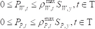
where S_W and S_P are the installed capacities of wind and PV, respectively, and and P_P,t represent their outputs at time t. The coefficients  and   denote the maximum output factors of wind and PV at time t.

Battery output constraints

   (11)

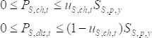
where P_{S, t} is the battery power (positive for discharge), while P_{S, ch, t} and P_{S, dis, t} represent charging and discharging power at time t, respectively.

Battery charging/discharging exclusivity

   (12)

where u_{S, ch, t} is a binary variable indicating battery charging status (1 for charging via the grid, 0 for discharging), and S_{S, P} denotes the rated power capacity of the battery.

Battery energy balance

   (13)

where E_S,t is the stored energy at time t, and η_ch and η_dis denote charging and discharging efficiencies, respectively.

Transmission power constraints

   (14)

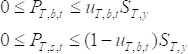
where P_T,b,t and P_T,s,t represent purchased and sold power through the transmission line at time t.

Transmission purchase/sales exclusivity

   (15)

where u_T,b,t is a binary variable indicating power purchase (1 for importing from the grid, 0 for exporting to the grid).

Energy balance constraint

   (16)

where P_L,t is the local load demand, and P_loss,t is the curtailed load at time t.

Minimum online capacity constraint

   (17)

where S_min,sys denotes the minimum required online capacity of local thermal units.

Minimum up/down time constraints

   (18)

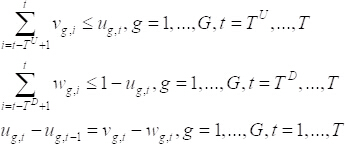
where v_g,t and w_g,t are binary variables indicating startup and shutdown of unit g at time t, and T^U and T^D denote the minimum up and down times of thermal units.

Determining production costs solely via day-ahead unit commitment is insufficient to capture flexibility challenges induced by forecast errors. It also fails to properly reflect the economic value of flexibility resources in ensuring secure and reliable operation.

Due to the inherent variability of wind and PV, net load experiences dynamic fluctuations during intraday operation. To address this, intraday regulation cost modeling is introduced to quantify the economic impacts of flexibility resources and their adequacy in mitigating deviations under uncertainty.

Figure 1 illustrates the concept of intraday adjustment and the associated adjustment costs. The horizontal axis represents the power. The light purple marker denotes the day-ahead forecast of net load, corresponding to the scheduled power generation and interchange. The actual intraday net load may deviate from this forecast, which is characterized by the cyan probability density curve. To accommodate these deviations, thermal units and tie-lines can be adjusted relative to the day-ahead schedule, indicated by the navy arrow and the pink arrow, respectively. The hatched shaded area highlights the portion of net load deviations that cannot be covered by the available adjustment capacity. Such uncovered deviations may lead to renewable energy curtailment or load shedding, which in turn affects energy balance and supply security while introducing additional risks and costs.

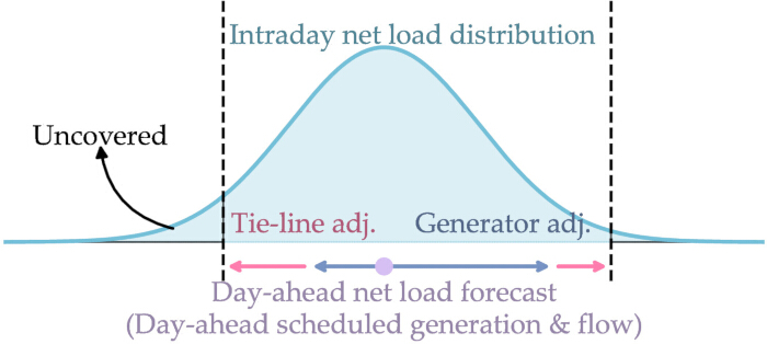
Figure 1: Illustration of day-ahead scheduling and intraday adjustment. Please click here to view a larger version of this figure.

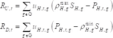
At time t, upward spinning reserve R_U,t and downward spinning reserve R_D,t are defined as:

   (19)

Forecast errors exist for wind, PV, and load. In general, load forecasts are generally more accurate, while PV forecasts exhibit greater error. When the load is overestimated and renewable output is underestimated, the system faces surplus power, requiring significant downward regulation. Conversely, underestimated load and overestimated renewable output result in supply shortages, necessitating substantial upward regulation.

To fully evaluate flexibility needs, two extreme scenarios are constructed: one dominated by upward regulation requirements and the other by downward regulation requirements. At time t, upward and downward flexibility demands L_U,t and L_D,t are expressed as:

   (20)

where σ_L, σ_W, and σ_P are constants determined by the forecast accuracies of load, wind, and PV, respectively.

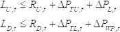
Upward flexibility is sequentially supplied by thermal generation, tie-line imports, and demand-side management, while downward flexibility is provided by thermal generation, tie-line exports, and renewable curtailment:

   (21)

Generating the samples

Obtain historical data: PV output, wind power output, load demand, and electricity price time series are downloaded from the open power system data repository²⁰. The timestamps and preprocess missing values are aligned using linear interpolation (interp1 function in MATLAB). Each parameter is divided into 15-min intervals, resulting in 96 data points per day for each variable.

Fit probability distributions: Beta distributions are fitted for PV output, Weibull distributions for wind output, normal distributions for load demand with embedded daily/seasonal cycles, and log-normal distributions for purchase and selling prices.

Generate scenarios using Latin hypercube sampling and importance sampling. The cumulative distribution of each parameter is divided into 20 equally probable intervals, and one value is sampled from each interval to form representative daily scenarios²³. LHS samples (50–100) are generated per parameter for robust coverage. IS is applied to oversample the top 10% and bottom 10% quantiles of forecast-error distributions to capture rare but critical events²⁴.

In this study, five sources of uncertainty are considered: PV output, wind power output, load demand, purchase price, and selling price. To appropriately represent the temporal variability and statistical characteristics of these uncertain parameters within the optimization model, probability distribution models are selected based on the historical observations and the physical attributes of each parameter. Sampling and scenario construction are subsequently performed according to these models.

Within this framework, a "scenario" is defined as a set of five time-series profiles—PV output, wind output, load, purchase price, and selling price—spanning an entire day and discretized at intervals of 15 min. By sampling each uncertain parameter and combining them, multiple representative daily operating conditions are generated. These scenarios are then used to simulate system operation under various stochastic perturbations, thereby enhancing the robustness and adaptability of the resulting planning decisions.

Regarding the choice of probability distribution models, PV output is typically modeled using Beta or Weibull distributions, capturing its skewness and saturation effects caused by variations in solar irradiance and cloud cover. Wind power output is generally represented by a Weibull distribution due to its strong dependence on stochastic wind speed fluctuations. Load demand is commonly assumed to follow a normal distribution, often with embedded periodic components to reflect daily and seasonal cycles. Meanwhile, purchase and selling prices, owing to their log-normal characteristics and occasional price jumps, are typically modeled using log-normal distributions.

Because a larger number of samples significantly increases the computational scale of the model and reduces solution efficiency, it is necessary to compress the sample set while retaining representativeness. To achieve this, two complementary sampling techniques are employed. First, Latin Hypercube Sampling is used to ensure more uniform coverage of the input space. Second, Importance Sampling is applied to oversample probability regions with higher operational significance, thereby improving the representation of rare but critical events.

Solving the model using nested generalized benders decomposition

MATLAB R2023a is opened, and the CPLEX 12.10 solver is configured. The sdpvar function in YALMIP is used to define all decision variables. The samples are generated in MATLAB according to the previous section. Each scenario is stored as a 5 × 96 matrix. The objective and constraints are formulated as YALMIP expressions, following the optimization model described in previous sections. For each scenario, the sequential production simulation subproblem is solved by calling the optimize function in YALMIP with CPLEX as the solver. Optimal solutions are extracted and dual variables are obtained calling the dual function to construct upper-level feasibility cuts²¹. The master problem is formulated and solved in YALMIP using the optimize function with CPLEX as the solver. Inner and outer loops are iterated. Alternatively, operational (y) and planning (z) decisions are updated by repeating the solving first level decomposition step, and it is repeated until the gap between upper and lower bounds²¹ is below a prescribed convergence tolerance 10^-6. The upper and lower bounds at each iteration are recorded for convergence monitoring.

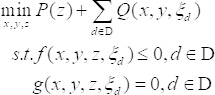
Detailed calculation formulas and further explanations of these steps are provided in the remainder of this section. Let the continuous variables in the scheduling problem be denoted by x, the integer variables by y, and the continuous variables in the planning problem by z. The scenario set is {ξ_d}_d∈D. Under each scenario, the original model can thus be expressed in the following compact form:

   (22)

where P represents the construction cost, while Q denotes the cost components related to unit commitment and dispatch.

The stochastic planning model is solved by a nested GBD²¹. GBD has been extensively applied to power system planning²⁵ and scheduling²⁶. Compared to heuristic algorithm²⁷, the nested GBD framework offers scalability and guaranteed convergence properties. Nested GBD extends the conventional GBD approach by introducing a multi-level subproblem structure.

In the first-level decomposition, a subproblem is constructed for each scenario. For a given scenario ξ_d and a given decision variable z = z^l, the sequential production simulation problem is formulated as:

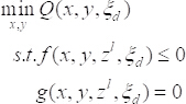   (23)

After solving the subproblems across all scenarios, an upper-level feasibility cut is generated as:

   (24)

where θ_u is an auxiliary variable introduced to represent the cost of the subproblem.

The master problem, representing the upper-level planning problem, remains:

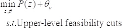   (25)

For each scenario ξ_d, the sequential operation simulation problem is further decomposed. The lower-level subproblem under a given y = y^k is a nonlinear programming (NLP) problem:

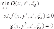   (26)

From its solution, a mid-level feasibility cut is derived as:

   (27)

where θ_m is an auxiliary variable introduced to represent the cost of the lower-level subproblem.

The mid-level master problem, corresponding to the integer programming layer, is then expressed as:

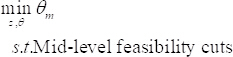   (28)

At the outer level, for a fixed planning decision z = z^l a per-scenario subproblem is solved to obtain optimal and duals; these produce upper-level feasibility cuts, where θ_u aggregates subproblem cost contributions. The outer master problem then updates z by minimizing P(z)+θ_u subject to the accumulated cuts.

For each scenario, the sequential operation simulation is itself decomposed by an inner GBD. Holding integer operational decisions y = y^k, the lower-level NLP is solved to yield primal/dual solutions and mid-level cuts, while the mid-level master updates integer y. The solution procedure alternates inner and outer loops: initialize l= 0, k = 0 with z⁰,y⁰, solve inner subproblems to generate mid/upper cuts, update masters to obtain y^k and z^l, and iterate. The optimal objective of the resolved subproblems provides an upper bound, and the master problems furnish a lower bound; convergence is declared when their gap is closed or below a prescribed tolerance. This nested GBD framework thus handles hierarchical decision layers and scenario coupling while retaining scalability and theoretical convergence guarantees. The overview of the protocol is shown in Figure 2.

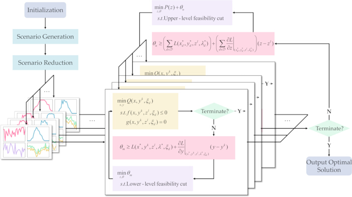
Figure 2: Overview of the proposed protocol. Please click here to view a larger version of this figure.

Results

Application of the proposed protocol generates representative planning and operational results that highlight the effectiveness of explicitly modeling intraday flexibility and carbon penalties.

Representative planning outcomes under carbon penalties

Using 400 representative scenarios across seasons, sequential production simulation produces the operational cost corresponding to each capacity expansion plan. Figure 3 pre...

Discussion

The presented protocol provides a life-cycle capacity planning framework that integrates sequential production simulation, intraday adjustment modeling, and nested generalized Benders decomposition to explicitly quantify the value of flexibility under intraday uncertainty. Unlike conventional capacity planning approaches that typically rely on deterministic formulations or simplified two-stage stochastic models^16,17, the proposed protocol explicitly embeds intrad...

Materials

List of materials used in this article

Name	Company	Catalog Number	Comments
Electricity market price data	Market operator / Open datasets	—	Day-ahead and intraday price inputs for operational cost modeling
Historical PV generation time-series data	Regional grid operator / Open datasets	—	Used for PV forecast modeling and scenario generation
Historical wind power time-series data	Regional grid operator / Open datasets	—	Used for wind forecast modeling and scenario generation
MATLAB / Python	MathWorks / Python Software Foundation	MATLAB R2025a / Python 3.11	Used to implement capacity planning model and sequential production simulation
Optimization solver (e.g., CPLEX, Gurobi)	IBM / Gurobi	CPLEX 22.1 / Gurobi 10.0	Solves the mixed-integer linear optimization problems
Scenario generation libraries	Python: pyDOE, NumPy, SciPy	pyDOE 0.3.1, NumPy 1.26, SciPy 1.11	Used for Latin Hypercube Sampling, importance sampling, and probability fitting
System load data	Regional grid operator / Open datasets	—	Used for load forecast and scenario generation
Visualization libraries	Python: Matplotlib, Seaborn	Matplotlib 3.8, Seaborn 0.12	Used to generate figures of planning results, operational trajectories, and reserve margins