This study developed and validated a depression risk prediction model for home-dwelling middle-aged and older adults using CHARLS data. This model incorporates five key predictive factors. The nomogram demonstrated acceptable discrimination (0.766/0.664), which is suitable for risk stratification at the population level and is an effective screening tool.
Research Article
Development and Validation of a Depression Risk Prediction Model for Home-Dwelling Middle-Aged and Older Adults in China Based on CHARLS Data
Opens in a new tab
In This Article
Summary
Loading...
$$\rightleftharpoonup{xx}$$
$$\longleftharp{xx}$$,
$$\longrightharp{xx}$$,
Abstract
Loading...
$$\rightleftharpoonup{xx}$$
$$\longleftharp{xx}$$,
$$\longrightharp{xx}$$,
There is a lack of research on risk prediction models for depressive symptoms among home-dwelling middle-aged and elderly adults in China. This study aimed to develop a risk prediction model and identify the risk factors for depression among home-dwelling middle-aged and elderly adults in China, with the goal of informing evidence-based prevention strategies and public health policy. Using the latest nationally representative CHARLS 2020 wave (n = 14,466), we developed the first parsimonious nomogram to predict depressive symptoms (CES-D-10 ≥ 10) in home-living middle-aged and older Chinese. After chi-square and multivariable logistic screens, LASSO with 10-fold cross-validation identified the five most influential predictors. Model discrimination (AUC), calibration (Hosmer-Lemeshow, calibration plot), and clinical utility (decision-curve analysis) were assessed in training–test splits (7:3). Among the 14,466 home-dwelling middle-aged and elderly adults, 5,488 (37.1%) had depressive symptoms, and 8,978 (62.9%) did not meet the criteria for depressive symptoms. The final nomogram comprised five variables: female sex, rural hukou, primary or less education, unmarried status, and age over 60. The tool achieved AUCs of 0.766 (95% CI 0.752-0.780) in the training set and 0.664 (0.637-0.691) in the test set, with excellent calibration (P = 0.28) and positive net benefit between 30% and 50% risk thresholds. This model can predict the risk of depression in Chinese home-dwelling middle-aged and elderly adults and can serve as a convenient screening tool for early identification and risk management of depression in this population.
Introduction
Loading...
$$\rightleftharpoonup{xx}$$
$$\longleftharp{xx}$$,
$$\longrightharp{xx}$$,
Depression, as a mental disorder characterized by high prevalence1, low treatment acceptance rates, and high recurrence rates, has become a major threat to the physical and mental health of middle-aged and elderly individuals2. Globally, it is estimated that 5% of adults suffer from depression, while among elderly adults this figure is approximately 30%3,4. In China, a recent study revealed that an estimated 50.6 million people are affected by depressive disorders, accounting for 17.8% of the global burden5. Zhu et al. reported that the incidence of depression ranges from 27.0% to 37.3% among elderly individuals in China6. In addition, under the comprehensive influence of aging and other factors, the mental health of older adults tends to deteriorate7. In China, the home-dwelling model was the main type of living and care model for middle-aged and elderly adults8. Investigating the prevalence of depression and its risk factors among middle-aged and elderly adults within this model is both essential and significant9.
Although previous research on depression among middle-aged and elderly people has covered many aspects, such as internet use10, sleep duration and quality11, physical pain12, etc., most of these are cross-sectional studies, mainly focusing on the association between the older adults of this group and depression and exploring its influencing factors13,14,15. Existing research suggests that living arrangements (home-based vs. institutional care) significantly affect depressive symptoms in middle-aged and elderly populations16,17. Some researchers also used models to develop prediction tools to assess the risk of depression among the elderly18,19. These studies, however, suffer from two major limitations: first, the existing prediction models are mostly developed for predicting depression risk in the general elderly population, lacking specific tools for home-dwelling middle-aged and older adults; and second, the clinical application of these results is insufficient.
Therefore, this study aims to construct a depression risk prediction model applicable to home-dwelling middle-aged and elderly adults in China using data from the 2020 CHARLS. To our knowledge, this represents the first parsimonious nomogram developed specifically for this population, distinguishing it from existing models that predominantly target the general elderly population without accounting for the influence of living arrangements. By analyzing this model, we sought to identify key risk factors, thereby providing a theoretical basis for developing targeted interventions. The model development was grounded in the stress-vulnerability framework, which posits that depression results from the interaction between demographic vulnerabilities and chronic stressors inherent in home-dwelling contexts20. This study is expected to contribute to the enhancement of mental health services, the development of targeted policies, and increased societal stability.
Access restricted. Please log in or start a trial to view this content.
Protocol
Loading...
$$\rightleftharpoonup{xx}$$
$$\longleftharp{xx}$$,
$$\longrightharp{xx}$$,
The research was approved by the Biomedical Ethics Committee of Peking University (IRB00001052-11015). All subjects provided informed consent.
Study population
The data for this study were obtained from CHARLS 2020, which covers 150 county-level units and 450 village-level units across the country, encompassing approximately 10,000 households and 19,395 middle-aged and elderly individuals aged 45 and above21. The survey employed a multi-stage probability sampling approach. Individuals were included if they met the following criteria: age of 45 years or older; selected home-dwelling in response to the questionnaire item BA007: What is the type of residence at the living address?; and provided a clear answer to the 10-item Center for Epidemiological Studies Depression Scale (CES-D-10). Individuals were excluded if they met one or more of the following criteria: responses indicating non-home residence (including communities, hospitals, and others or missing); lack of information on depression; lack of information on relevant covariates. Ultimately, 14,466 adults who met the initial criteria were included in this study. The detailed process of participant selection is illustrated in Figure 1.
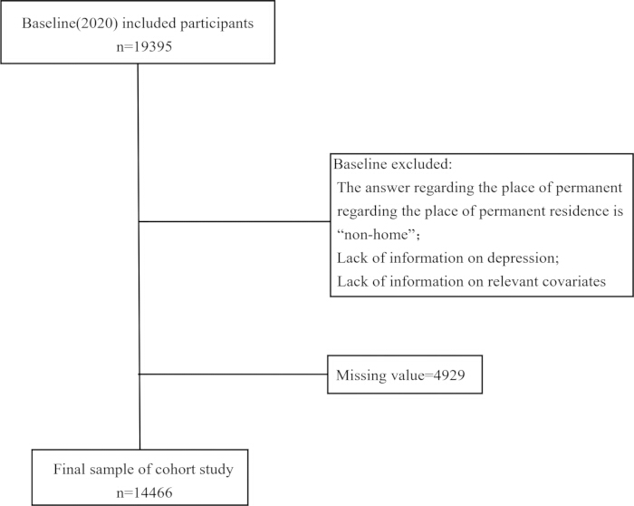
Figure 1: A flow chart for study population selection. Please click here to view a larger version of this figure.
Definition of the variables
Depressive symptoms were assessed using a simplified version of the CES-D-10, which has high reliability and validity in previous studies22,23. The CES-D-10 has 10 items with four scales: 0 = never, 1 = sometimes or rarely, 2 = often, and 3 = always, and the fifth and eighth items are scored in reverse24. The total score of the depression scale is obtained by summing the ratings of all 10 items, ranging from 0 to 30; the higher the score, the more serious the individual’s depressive symptoms. Based on previous studies of middle-aged and elderly populations25,26, participants with CES-D-10 scores ≥10 were classified as having depressive symptoms, whereas scores <10 were classified as non-depressed.
Information collected from all study participants includes demographic information (age, gender, marital status, residence, and education level), living habits and physical health status (physical activity, smoking, drinking, social interactions, self-rated health, the status of chronic disease, and nap time), and information related to living conditions and children (satisfaction with living conditions, the marital status of the offspring, and the health status of the offspring). Chronic diseases are diagnosed by doctors and include hypertension, dyslipidemia, malignant tumors, chronic lung disease, heart disease, stroke, arthritis, and rheumatism.
Statistical analysis
Binary logistic regression analysis
Categorical variables are presented as frequencies and percentages. Chi-square tests were conducted to examine differences in depression incidence across various demographic characteristics within the study population. Binary logistic regression analysis was performed to identify significant factors associated with depressive symptoms. These statistical analyses were performed using SPSS software (version 21.0).
LASSO regression
In R version 4.3.2, the dataset was randomly partitioned into a training set and a test set at a 7:3 ratio using a fixed random seed to ensure reproducibility. Specifically, 70% of the data were allocated to the training set for model development, and 30% to the test set for independent validation. First, variables that were statistically significant (p < 0.05) in the binary logistic regression were included in the LASSO regression analysis to prevent overfitting by shrinking the coefficients. The optimal lambda value was determined via 10-fold cross-validation. The lambda.1se was selected based on the one standard error rule to achieve the optimal variable selection performance. LASSO shrinkage was employed to prevent overfitting by reducing the coefficients of less important variables toward zero. For further details, please consult the Supplementary File 1 (item 1).
Nomogram construction
The relative importance of the selected predictors was ranked according to the absolute magnitude of their standardized coefficients and visualized using a forest plot. A predictive nomogram was constructed using the rms package, based on the final logistic regression equation. For further details, please consult the Supplementary File 1 (item 2).
Model validation
Discrimination was evaluated by calculating the area under the receiver operating characteristic curve (AUC) using the pROC package. The AUC was calculated separately for the training set and test set. Typically, an AUC greater than 0.75 indicates good discrimination. For further details, please consult Supplementary File 1 (item 3).
Calibration: Model calibration was assessed using the Hosmer-Lemeshow goodness-of-fit test and visualized with calibration curves generated by the rms package, plotting predicted probabilities against observed frequencies. A non-significant Hosmer-Lemeshow test (p > 0.05) indicates good calibration. For further details, please consult the Supplementary File 1 (item 4).
Clinical utility: Clinical utility was evaluated using decision curve analysis (DCA) with the rmda package, calculating net benefit across threshold probabilities from 0% to 100%. For further details, please consult the Supplementary File 1 (item 5).
Random forest validation: As a supplementary validation, a random forest model was implemented using the randomForest package to assess model stability and generalizability. The error rate convergence curve was plotted to evaluate the relationship between the number of trees and prediction accuracy in both training and test sets. A two-sided p value < 0.05 was considered to indicate a statistically significant difference. For further details, please consult the Supplementary File 1 (item 6).
Access restricted. Please log in or start a trial to view this content.
Results
Loading...
$$\rightleftharpoonup{xx}$$
$$\longleftharp{xx}$$,
$$\longrightharp{xx}$$,
Sample characteristics
The study comprised 14,466 participants with the following characteristics: 46.8% were aged 60-74 years, 52.2% were female, and 75.2% held agricultural household registration status. In terms of educational level, 62.9% had a primary school education or lower. Regarding mental health status, 37.1% of participants exhibited depressive symptoms, while the remaining 62.9% showed no depressive symptoms. Detailed information was presented in Table 1.
Access restricted. Please log in or start a trial to view this content.
Discussion
Loading...
$$\rightleftharpoonup{xx}$$
$$\longleftharp{xx}$$,
$$\longrightharp{xx}$$,
This study yielded several key findings regarding the risk factors and prediction of depressive symptoms among home-dwelling middle-aged and elderly adults in China. First, the study found that 37.1% of home-dwelling middle-aged and elderly adults exhibited depressive symptoms in China, indicating a high burden of depressive symptoms in this population. The results of this study were inconsistent with the findings of a global meta-analysis on the prevalence of depressive symptoms in older adults, which reported a figure ...
Access restricted. Please log in or start a trial to view this content.
Disclosures
Loading...
$$\rightleftharpoonup{xx}$$
$$\longleftharp{xx}$$,
$$\longrightharp{xx}$$,
None declared.
Acknowledgements
Loading...
$$\rightleftharpoonup{xx}$$
$$\longleftharp{xx}$$,
$$\longrightharp{xx}$$,
This study was supported by the Social Science Planning Project of Jiangxi Province (20SH17) and the Science and Technology Project of the Jiangxi Education Department (GJJ191063 and GJJ171078). Sincerely, thanks to the National School of Development at Peking University and the Institute of Social Science Survey for providing the related data. Author contribution: Conceptualization, X.X.Z. and J.X.X.; methodology, J.X.X. and S.G.Z; software, X.X.Z.; validation, J.X.X. and S.G.Z.; formal analysis, S.G.Z. and R.J.W.; investigation, J.X.X. and W.C., B.B.D. and L.B.L.; resources, J.X.X., S.G.Z., W.C., B.B.D. and L.B.L.; data curation, J.X.X. and S.G.Z; writing—original draft preparation, J.X.X. and S.G.Z; writing—review and editing, X.X.Z., J.X.X., S.G.Z., R.J.W., X.J.L, Y.T.X, R.L, and W.J.H.; supervision, X.X.Z. Funding acquisition, X.X.Z. All authors have read and agreed to the published version of the manuscript.
Access restricted. Please log in or start a trial to view this content.
Materials
| Name | Company | Catalog Number | Comments |
|---|---|---|---|
| (pROC)(shapviz)(patchwork)(xgboost)(ggplot2)(rms)(rmda)(caret)(randomForest)(glmnet)(dplyr)(ggrepel)(readr) | CRAN | N/A | R package for risk prediction model decision curve analysis |
| CHARLS dataset | CHARLS team | N/A | China Health and Retirement Longitudinal Study dataset, used for model development and validation |
| R | R Foundation for Statistical Computing | 4.3.2 | Statistical software used for data analysis and modeling. |
| SPSS Statistics | IBM | 21 | Software used for supplementary statistical analysis. |
References
Loading...
$$\rightleftharpoonup{xx}$$
$$\longleftharp{xx}$$,
$$\longrightharp{xx}$$,
- Herrman, H., et al. Reducing the global burden of depression: a Lancet-World Psychiatric Association Commission. Lancet. 393 (10174), e42-e43 (2019).
- König, H., König, H. H., Konnopka, A. The excess costs of depression: a systematic review and meta-analysis. Epidemiol Psychiatr Sci. 29 (1), e30(2019).
- Cai, H., et al. Global prevalence of depression in older adults: a systematic review and meta-analysis of epidemiological surveys. Asian J Psychiatr. 80, 103417(2023).
- Hu, T., et al. Prevalence of depression in older adults: a systematic review and meta-analysis. Psychiatry Res. 311, 114511(2022).
- Hu, X., Jin, W., Wang, J., Dong, H. Age, period, cohort effects in trends of depressive symptoms among middle-aged and older Chinese adults. Front Public Health. 12, 1383512(2024).
- Zhu, L., et al. Depressive symptoms and all-cause mortality among middle-aged and older people in China and associations with chronic diseases. Front Public Health. 12, 1381273(2024).
- Cui, L., et al. Factors affecting the evolution of Chinese elderly depression: a cross-sectional study. BMC Geriatr. 22 (1), 109(2022).
- Liang, S., Zhou, M., Zhou, C., Zhu, J., Tosi, F. Existing Chinese Elderly Care Service Models and Their Development Based on Literature Review. J Packaging Engineering. 43 (22), 408-417 (2022).
- Wu, H., et al. An investigation into the health status of the elderly population in China and the obstacles to achieving healthy aging. Sci Rep. 14 (1), 31123(2024).
- Du, X., Liao, J., Ye, Q., Wu, H. Multidimensional Internet Use, Social Participation, and Depression Among Middle-Aged and Elderly Chinese Individuals: Nationwide Cross-Sectional Study. J Med Internet Res. 25 (12), e44514(2023).
- Dong, J., et al. Depressive symptoms among middle-aged and older adults in China: the interaction of physical activity and sleep duration. Sleep Health. 11 (2), 214-221 (2025).
- Bao, M., Ma, R. Longitudinal relationship between adverse childhood experiences and depressive symptoms: the mediating role of physical pain. BMC Psychiatry. 24 (1), 947(2024).
- Liu, G., Zhang, J. Association of a novel nutritional index with cognitive impairment in middle-aged and elderly Chinese adults: a cross-sectional analysis from the China Health and Retirement Longitudinal Study. Front Nutr. 12, 1486917(2025).
- Ai, Z., Tang, C., Wen, X., Kartheepan, K., Tang, S. Examining the impact of chronic diseases on activities of daily living of middle-aged and older adults aged 45 years and above in China: a nationally representative cohort study. Front Public Health. 11, 1303137(2023).
- Lu, J., Ruan, Y. Exploring the reciprocal relationship between depressive symptoms and cognitive function among Chinese older adults. Healthcare (Basel). 11 (21), 2880(2023).
- Chen, F., Short, S. E. Household Context and Subjective Well-Being Among the Oldest Old in China. J Fam Issues. 29 (10), 1379-1403 (2008).
- He, W., et al. Quality of life of empty-nest elderly in China: a systematic review and meta-analysis. Psychol Health Med. 25 (2), 131-147 (2020).
- Gao, S., Zhang, H. Development and validation of a depression risk prediction model for rural elderly living alone. BMC Psychiatry. 25 (1), 357(2025).
- Zheng, Y., Zhang, C., Liu, Y. Risk prediction models of depression in older adults with chronic diseases. J Affect Disord. 359, 182-188 (2024).
- De Beurs, E., et al. On becoming depressed or anxious in late life: similar vulnerability factors but different effects of stressful life events. Br J Psychiatry. 179 (5), 426-431 (2001).
- Bai, Q., et al. Configurational effects of intergenerational support on older adults' depression: an empirical study from CHARLS data. BMC Public Health. 25 (1), 392(2025).
- Wang, C., Huang, Z., Lu, Z., Wang, P. Social Interaction as a vital factor in alleviating depressive symptoms among middle-aged and elderly adults: evidence from the CHARLS. Aging Clin Exp Res. 37 (2), 115(2025).
- Lei, X., Sun, X., Strauss, J., Zhang, P., Zhao, Y. Depressive symptoms and ses among the mid-aged and elderly in china: Evidence from the china health and retirement longitudinal study national baseline. Soc Sci Med. 120, 224-232 (2014).
- Jiang, X., et al. Efficacy of nondrug interventions in perinatal depression: a meta-analysis. Psychiatry Res. 317, 114916(2022).
- Xu, Y., et al. Decomposing socioeconomic inequalities in depressive symptoms among the elderly in china. BMC Public Health. 16 (1), 1214(2016).
- Yang, Y., Hou, D. L. Association of depressive symptoms and dementia among middle-aged and elderly community-dwelling adults: results from the China Health and Retirement Longitudinal Study (CHARLS). Acta Psychol (Amst). 243, 104158(2024).
- Piovani, D., Sokou, R., Tsantes, A. G., Vitello, A. S., Bonovas, S. Optimizing Clinical Decision Making with Decision Curve Analysis: Insights for Clinical Investigators. Healthcare. 11 (16), 2244(2023).
- Ndapatani, L., et al. Cervical cancer screening and treatment of VIA positive lesions among women living with HIV in Nairobi and Kajiado counties, Kenya: results from a targeted intervention implemented under the USAID Fahari ya Jamii project in supported HIV clinics. BMC Women's Health. 25, 621(2025).
- Yan, R., et al. Association between internet exclusion and depressive symptoms among older adults: panel data analysis of five longitudinal cohort studies. EClinicalMedicine. 75, 102767(2024).
- Surya, J., Kashyap, H., Nadig, R. R., Raman, R. Developing a Risk Stratification Model Based on Machine Learning for Targeted Screening of Diabetic Retinopathy in the Indian Population. Cureus. 15 (9), e45853(2023).
- Baldini, V., et al. A comprehensive approach to adolescent suicide prevention: insights from a narrative review perspective. Front Psychol. 16, 1612067(2025).
- Li, H., Liu, X., Zheng, Q., Zeng, S., Luo, X. Gender differences and determinants of late-life depression in China: a cross-sectional study based on CHARLS. J Affect Disord. 309, 178-185 (2022).
- Parker, G., Brotchie, H. Gender differences in depression. Int Rev Psychiatry. 22 (5), 429-436 (2010).
- Acciai, F., Hardy, M. Depression in later life: a closer look at the gender gap. Soc Sci Res. 68, 163-175 (2017).
- Choi, S. E., Zhang, Z. Caring as curing: Grandparenting and depressive symptoms in China. Soc Sci Med. 289, 114452(2021).
- Nguyen, A. W., Walton, Q. L., Thomas, C., Mouzon, D. M., Taylor, H. O. Social support from friends and depression among African Americans: the moderating influence of education. J Affect Disord. 253, 1-7 (2019).
- Ling, Y., Song, Z., Yu, Y., Jiang, T. Dealing with an aging China-Delaying retirement or the second-child policy. PLoS One. 16 (12), e0242252(2021).
- Bedaso, T. S., Han, B. Work after retirement affects elderly mental health and behaviors in Addis Ababa. Health Psychol Open. 8 (2), 2055102921996189(2021).
- Chen, F., Liu, G. The health implications of grandparents caring for grandchildren in China. J Gerontol B Psychol Sci Soc Sci. 67 (1), 99-112 (2012).
- Thomeer, M. B. Multiple Chronic Conditions, Spouse's Depressive Symptoms, and Gender within Marriage. J Health Soc Behav. 57 (1), 59-76 (2016).
- Toshishige, Y., et al. Association between marital satisfaction of female patients with persistent depressive disorder, and their own and husbands' autism spectrum disorder or attention deficit/hyperactivity disorder traits. PCN Rep. 2 (2), e95(2023).
- Guo, J., et al. Depression among Chinese older adults: A perspective from Hukou and health inequities. J Affect Disord. 223, 115-120 (2017).
- Saravanakumar, P., Muhammad, T., Paul, R., Srivastava, S. Explaining the Urban-Rural Difference in Late-Life Depression in India: Evidence from a Multivariate Decomposition Analysis Based on Longitudinal Aging Study in India, Wave 2017-18. Clin Gerontol. 47 (2), 270-287 (2024).
- Gao, Q., et al. Exploring the interplay of living arrangements, social support, and depression among older adults in rural northwest China. BMC Public Health. 24 (1), 3297(2024).
Access restricted. Please log in or start a trial to view this content.
Reprints and Permissions
Request permission to reuse the text or figures of this JoVE article
Request Permission