Translating Professional Football Helmet Tests to Full Body Finite Element (FE) Simulations: A Reproducible Field-to-Simulation Workflow

Summary

This article presents a reproducible workflow that converts real national football league (NFL) plays into solver-ready full-body finite element simulations. Single-view video reconstructs 6-DoF skull-CG kinematics, applies event-specific helmet hardware, and enforces quality-control gates for stability, energy balance, and driver fidelity to support cross-lab reproducibility without injury claims.

Abstract

This article presents a reproducible field-to-simulation workflow that translates real football plays into solver-ready boundary conditions for a full-body finite-element human model. Single-view video reconstructs six-degree-of-freedom kinematics at the skull CG; these signals are applied to a helmet–head–body assembly that preserves event-specific hardware. The protocol codifies quality-control gates before interpretation: (I) helmet readiness (mesh integrity, contact stability), (ii) mass and center-of-gravity agreement between the physical configuration and its FE surrogate, (iii) energy balance with bounded spurious energies, (iv) driver-fidelity metrics comparing target versus solver-applied motion (RMSE, peak magnitudes, time-to-peak), and (v) versioned inputs for auditability. A demonstration replay verifies numerical stability and driver fidelity, and reports tissue-level response and diagnostic damage metrics as process outputs without making injury claims. For studies requiring internal response, the framework supports physics-based constitutive models (Internal State Variable formulations) and treats them as process diagnostics unless separately validated. By separating readiness checks from injury interpretation, the method provides a practical foundation to standardize helmet integration, enable cross-laboratory reproducibility for event scenarios, and inform safer design and policy. Although developed for sport, the workflow generalizes to transportation and defense settings where ethical constraints prevent human experimentation.

Introduction

The goal of this end-to-end reconstruction method is to represent real-world player impacts by converting field evidence (video and/or wearables) into a simulation-ready human–helmet assembly. The protocol provides procedural steps and quality-control gates to integrate a legacy football helmet with a whole-body finite-element (FE) human model and to enable event-specific simulations that can later be analyzed for safety insights. Head impacts in contact sports highlight a key limitation of controlled league laboratory programs^1,2,3,4. NOCSAE certification^5,6,7,8,9,10 and the league laboratory linear impactor protocol^11,12 benchmark products under canonical conditions. However, by design, they do not reconstruct the event-specific details of on-field collisions or require full system configurations. Stiffness couplings within the assembled helmet (facemask–shell–mounts) can materially change the response and are not captured in these standardized setups^{1,12,13,14,15}.

Here, a process-only workflow carries a real incident from raw observation to an FE assembly: tracing helmet specification, building the helmet model, fitting and constraining it to a whole-body human model (full-body FE human model; Table of Materials), defining contacts and boundary conditions^16,17, and executing a low-severity demonstration input to certify simulation readiness. This method provides a practical foundation to standardize helmet integration and promote reproducibility for non-ideal, event-specific scenarios—serving as the groundwork upon which future simulations can support comparative helmet evaluation and safety research^18,19,20,21. The workflow applies to helmet use beyond professional football (youth/collegiate play and other helmeted activities) when comparable multi-view video or test kinematics are available.

Reconstructing a real play for computational replay requires the six degrees of freedom (6-DOF) motion of the head center of gravity (CG)²²: three translations x, y, z, and three rotations (yaw, pitch, roll). In practice, head pose is estimated from single-view video by tracking rigid helmet landmarks and solving a zoom-aware PnP (UPnP)^23,24 pose per frame using a known 3D helmet landmark template; focal length is estimated per frame, and the resulting skull-CG 6-DOF time histories are used as initial boundary value conditions inputs. The resulting 6-DOF profile becomes the driver applied at the skull CG of the finite-element (FE) human. These include root-mean-square error (RMSE) over the time window of interest and feature deltas (peak magnitude and time-to-peak differences for angular velocity/acceleration). Reporting these measures sets up that any downstream model response is conditioned on a well-reproduced kinematic history. Before any interpretation, the assembly must meet simulation-readiness criteria: (i) mesh quality thresholds for all helmet and head components; (ii) mass/CG agreement between the physical helmet configuration and its FE surrogate; (iii) energy balance with bounded hourglass energy and stable contact energy; (iv) contact stability (zero initial penetrations, no chatter, penetration within a small tolerance); and (v) the input fidelity metrics above. These gates certify that the model is numerically sound and that the replayed event is a faithful reproduction of the reconstructed motion.

Internal injury is critical for real player impacts; therefore, a physics-based Internal State Variable (ISV) formulation was used to capture large-deformation, rate-sensitive, and history-dependent brain response, with an additional ISV term used as a diagnostic damage variable. This approach was adopted to move beyond purely kinematic injury criteria²¹ and to report a biology-relevant damage surrogate. Here, “damage” refers to regions of tissue-level microstructural disruption that are associated with sites where tau protein accumulation may occur. The original implementation captures the large-strain deformation behavior of polymers with three ISVs reflecting small-strain elasticity, softening, and large-strain hardening^25,26. A detailed description of the polymer ISV is provided in the supplementary material. The model was calibrated to compressive quasi-static and high-rate behavior of porcine brain^27,28. The model was validated by reproducing the coup/contrecoup intracranial pressure time histories measured in cadaver head-impact experiments using FE simulations^28,29. Empirically, brain shows similar constitutive behavior in compression and simple shear at matched rates (Figure 1); the model reproduces low-rate compression (Figure 2) and after adding a damage tracker aligns with high-rate (30–60 s⁻¹) compression datasets (Figure 3).

The model²⁵ was extended by incorporating a damage term to model pore growth resulting from stress triaxialities (tensile pressure) and shear strains. The term “damage” here refers to the total volume fraction of damaged brain material, which stands for lower-length scale structures. The term lower-length scale structures refers to sub-macroscale damaging or inflammatory response artifacts, such as tau protein and tau protein accumulation³⁰. Pore growth from the stress triaxiality is captured with the Cocks and Ashby²⁹ pore growth rate equation:

(1)

where Φ_pore is the volume of the damaged brain, m_CA is the Cocks and Ashby damage exponent, I₁ is the first stress invariant related to hydrostatic pressure,I₂ is the second deviatoric stress invariant related to the effective stress, D_p and is the plastic rate of deformation tensor. Though originally formulated for metals, the Cocks and Ashby equation (1) was suitable for modeling pore growth in polymers³¹.

Due to its high-water content, the brain is particularly susceptible to shear stress²⁷. The Cocks and Ashby²⁹ pore growth model captures the hyperbolic relationship between tensile pressure and pore growth, not the influence of shear strains. An additional term must be added to account for the influence of shear strains on pore growth to make it suitable for use in soft materials. The model also introduced a pore growth sensitivity from shear stresses³²:

(2)

where I₃ is the third deviatoric stress invariant, is the deviatoric rate of deformation tensor, and σ'_ij is the deviatoric Cauchy stress tensor. K_pore is a scalar modifier to the Lode angle function (ω(σ)) and the deviatoric portion of the stress tensor, hence, it is the shear sensitivity parameter. The Lode angle function describes the state of stress in a material, particularly the stress triaxiality and the deviatoric stress components. The Lode angle function^{28,29,30,31,32,33}, ω(σ), is expressed as the following:

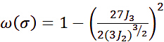(3)

Here the σ is the Cauchy stress tensor. Finally, the total damage growth from stress triaxialities and shear strain is calculated by adding the individual contributions from tensile pressure (Equation 1) and shearing (Equation 2) as follows:

(4)

where Φ_pore  is the total pore growth rate, combining the effects of hydrostatic tension and shear deformation. Details of the head and helmet mesh are given in Table 1. Each element in the finite-element (FE) brain mesh is assumed to have an initial pore volume fraction of . For reference, the average characteristic length and volume of a hexahedral element in the 3D FE mesh of the human brain used later in this paper are 2.6 mM and 2.07 mM³, respectively. An initial damage level (pore volume fraction) of corresponds to a pore radius of 0.0079 mM (7.9 µM) and a pore volume of mm³, well below the visible resolution of any current MRI or CT scanner³¹. The full constitutive model contains 22 material parameters (Table 2). Within the CAVEMAN head model, the ISV material formulation is applied to both white and gray matter of the patient-specific head form. The prescribed six-degree-of-freedom (6-DOF) motion at the skull center of gravity provides boundary kinematics, and the solution returns the stress–strain fields , internal and contact energies, and evolving internal state variables (ISVs) over time. Calibration and validation of the base constants, including m_CA and K_pore , follow established procedures, and are assumed to be known for this study.

Protocol

1. Helmet preparation (FE surrogate ready for coupling)

1. Identify configuration.
2. Open LS-PrePost and Import selected the helmet FE surrogate with faceguard and hardware matching the event configuration.
   1. Record padding set/size and chinstrap routing; Note solver/model versions: LS-PrePost³⁴ and Velodyne¹⁶.
3. Sanity-check mass properties.
   1. In LS-PrePost, open measurement and set the dropdown item menu to mass. Use 3-pt radius to define the helmet datum and report the helmet CG relative to that datum. Record the FE helmet mass (target: 1.82 ± 0.5 kg), CG, and overall dimensions.
4. QC Gate (needed for reproducibility).
   1. Do not continue unless the helmet mass and CG are within the acceptance range (mass target above; CG within your defined tolerance relative to the datum).
5. Verify mesh and interfaces.
   1. Verify the helmet mesh is hex-dominant. Remove wedge elements if present using LS-PrePost select element editing, select wedges, Delete, before hitting accept, ensure only wedge elements have been deleted and no additional elements were selected, Accept.
   2. On the Corvid HPC, convert the helmet keyword file to Velodyne binary geometry/sets using ls2vel+. Example:
      1. In terminal: ls2vel+ helmet.k (Replace helmet.k with the actual helmet keyword filename.)
      2. Confirm internal interface definitions required for the helmet are present and correct (pads, pad–pad, facemask mounts, strap anchors).
6. Helmet-only stability check (“shake”) 1–2 ms (QC gate).
   1. Create a helmet include keyword file (e.g., helmet_H1.k) and place it in the run directory. In velodyne.card, add an include line referencing helmet_H1.k. Place this include before any contact/friction definitions that reference helmet part IDs.
   2. The part number for the helmet system should be as follows:
      1. Helmet 1 parts begin at 10,000,000.
      2. Helmet 2 parts begin at 20,000,000.
   3. Select the renumber option and import the helmet 1 or helmet 2 renumbering, review the new numbering system, and accept.
   4. For renumbering head to Model and Part, renumber, select the All option, and in the start ID record either 20 or 10 million, then set, review the updated numbering system, and select renumber to confirm.
   5. Use the same solver/contact controls intended for the full run, but shorten the run to a quick stability window:
      1. Set Termination time: 1.0E−03 s (1 ms).
      2. Apply an initial velocity in the x direction to the whole helmet part set (20000000–29999999 or 10000000–19999999). Refer to step 3 for initial velocity setup. Use 40 cm/s as the input.
   6. Submit the card file using sbatch submit.slurm.sh.
   7. Confirm stability (no negative volumes; no contact blow-ups).
      1. The run completes without solver termination.
      2. No negative volume errors occur.
      3. No contact instabilities (“blow-ups”) appear in the solver log/output.
      4. The explicit stable time step does not collapse below a floor (e.g., Δt_min ≥ 1×10⁻⁷ s), based on the timestep output/log.
7. Visualization-based QC in VisIt (required for acceptance)
   1. In a terminal, navigate to the plot output directory: plot_directory/plot_files/.
   2. Launch VisIt: visit in a new command window.
   3. In VisIt, open the plot database/files: File, Open (select the files in plot_files).
   4. Create a von Mises stress plot: Add, Pseudocolor, Solid, Von_mises criterion, Draw.
   5. Look through output files (status.timstep, and plot_files), reject the run if you observe:
      1. Explosive/nonphysical deformation (elements “spiking”/collapsing).
      2. Sudden rigid-body or unrealistic launches.
      3. Rapidly growing stress singularities that spread.

2. Video and 6-DOF acquisition (target driver generation).

1. Bring videos under versioned control.
   1. Import a single-view video and log frame rate and resolution into Kinovea³⁵.
2. Define landmarks and digitize frames.
   1. Use rigid triad: LM1 facemask center; LM2/LM3 left/right facemask. Note: Shell screws are allowed if LM1-3 is blocked (or earholes if screws occlude).
   2. Digitize landmarks per frame (2D clicks). For each usable frame, click LM1–LM3 (and any additional visible rigid helmet landmarks) using the cursor. Record the pixel coordinates for every click and export a CSV named kinovea_clicks.csv with columns: frame, landmark_id, u_px, v_px.
3. Single-view pose and 6-DOF reconstruction (zoom-aware UPnP)^23,24.
   1. Provide the 3D helmet landmark template in meters as helmet_landmarks.csv (landmark, X, Y, Z) and a configuration file Config.json (fps, principal point, filter cutoffs, helmet_to_com).
   2. Open a command window and navigate to the file location for creconstruct_6dof_unpnp.py.
   3. Run: python reconstruct_6dof_upnp.py --clicks kinovea_clicks.csv --landmarks helmet_landmarks.csv --config.json³⁶.
   4. Use the exported files poses_per_frame.csv, kinematics.csv, and initial_conditions_t0.csv as the reconstruction outputs.
   5. NOTE: No lens distortion model was used. The principal point was assumed at the image center (c_x = 640, c_y = 360), focal length was estimated per frame, and smoothing cutoffs were applied (linear 15 Hz, angular 40 Hz; focal 5 Hz).
4. Impact reference and export.
   1. Set t₀ at peak angular acceleration of the struck head; report peak linear and angular accelerations.
   2. Export the initial conditions from initial_conditions_t0.csv for solver initialization (linear and angular velocities + orientation).
   3. Checkpoint (QC gate): median reprojection RMSE ≤ 8 p_x (0 frames > 8 p_x); focal-length drift ≤ 3.0%; landmark baseline drift ≤ 6%.

3. Simulation set up using helmets and CAVEMAN models.

1. Mount helmet on CAVEMAN head.
   1. Load CAVEMAN [v25p5] in Velodyne; seat the helmet; eliminate initial penetrations using element projection¹⁷, if needed, also use element editing to get sufficient fitting of the helmet to the skin head form.
2. Define helmet–head contact friction (Velodyne)
   1. Use the skin/fat layer part as the head-side friction partner (patient-specific CAVEMAN commonly uses PID 60009020: 60009020_O_Skin_FatLayer_Genderless). If the run uses a different head-contact part, record that PID and use it in Step iii.
   2. In the helmet setup include (velodyne.card), add/verify the helmet–skin friction type definition (Friction Type ID 2, Type 0) with the coefficients used:
      1. friction type definition: 2.
      2. 0.5 0.5
   3. In the helmet include, create part sets for pad groups. Keep the pad-set IDs stable so friction is not affected:
      1. Part set definition: 10000099 10000174 10000180 H1_pads_set1.
      2. Part set definition: 10000100 10000184 10000194 H1_pads_set2.
   4. If the helmet uses different pad PIDs, update the PID ranges (or list the exact pad PIDs) and record them.
   5. Activate helmet–skin friction pairs by uncommenting (or adding) the friction pair definitions. Add the following to any file or line included in the velodyne.card file.
   6. Friction pair definition:
      1. 60009020 10000099 1 exteriorfric! H1_pads_set1_to_skin.
      2. 60009020 10000100 1 exteriorfric! H1_pads_set2_to_skin.
      3. 60009020 10000181 2 exteriorfric! H1_Chincup_to_skin.
   7. For the second helmet, repeat using the Helmet-2 pad set IDs and chin cup PIDs if the two-helmet setup uses those.
3. Simulation controls.
   1. In the velodyne.card, set the Global Simulation Controls using the keyword definitions below.
      1. Solution Type: 0.
      2. Type 0 here is for Explicit structural.
      3. Global memory size: 32.
      4. Initial memory allocation in Gbyte.
      5. Termination time: 30.0E-03 s. (30 ms)
      6. Time step scale factor: 0.900.
      7. Plot state frequency: 1.0E-03 0.
      8. Plots the simulation output at the current state with a frequency of 1E-3 ms for a constant interval of the simulation.
      9. Time history frequency: 1E-03 0.
   2. Set global hourglass stabilization for reduced (single point) integration elements.
      1. In the velodyne.card, set hourglass stabilization to stiffness form, and specify the coefficient using the keyword definitions below:
      2. Hourglass stabilization method: 4.
      3. Hourglass stabilization coefficient: 0.10.
      4. Do not apply part-specific HGID overrides for hourglass control.
   3. Set global bulk viscosity for shock capture.
      1. In the velodyne.card, set:
      2. Bulk viscosity: 1.
      3. Quadratic bulk viscosity: 1.2.
      4. Linear bulk viscosity: 0.06.
   4. Enable mass scaling and define for all parts.
      1. Set: Part Set Definition: 99 1 899999999 All_parts_in_range.
      2. Mass scaling timestep: 1.92E−07.
      3. Mass scaling restart option: 1.
      4. Mass scaling part definition: 99 1.
   5. Set global contact controls (all materials).
      1. Contact scheme: 3 !(Lagrange multiplier).
      2. Curvature based adaptive contact option: 3 !(center + corners).
      3. Contact constraint type: 0 ! (velocity constraint).
      4. Max number of contact iterations: 20.
      5. Contact convergence tolerance: 1.00E−03.
4. Boundary conditions and controls
   1. Load LS-PrePost, import a single player setup (Helmet mesh and Full-body player mesh).
   2. In Keyword Manager, create one Part Set that includes all player parts currently loaded, and assign it a single Part Set ID (PSID) (use this PSID for the driver/initial-velocity definitions).
   3. Import the reconstructed 6-DOF kinematics CSVs and map them to the impactor/approaching player rigid body/part set; verify the global axes and initial orientation match the reconstruction reference frame before applying the initial velocity.
5. Keep the impacted player unconstrained (no prescribed motion or fixed supports). Initialize them in the desired nominal/posed starting posture at and allow their motion to be governed by contact and inertia during the replay.
6. Applying extracted kinematics (Velodyne Initial velocity definition).
   1. Add the linear and angular velocities like in Table 3 using Velodyne’s Initial Velocity definition keyword (PSID = player part set ID; styp = 1 for PSID). Use the same reference orientation definition line following each entry. Example syntax to add into velodyne.card:
      1. Initial velocity definition: <Part Set ID> 1 <V_x> <V_y> <V_z> <omega>
      2.  < P_x> < P_Y> < P_z > < Q_x > < Q_z >
      3. When used, the linear velocities are globally defined, while the omega will be defined by an axis defined by the two points P and Q defined by the researcher.
   2. To extract the points P and Q for correct angular acceleration assignment,
      1. Import the Skin shell Mesh for the specific player being assigned the angular Velocity (60009020_O_Skin_FatLayer_Genderless.k or 40009020_O_Skin_FatLayer_Genderless.k) into LS-PrePost.
      2. Define in 3D space the best axis that will define the rotational axis for the angular velocity.
      3. Apply the points to the prescribed first velocity definition above.
7. Execute the run by using sbatch submit.slurm.sh for the newly updated velodyne.card file while in the same file directory.
   1. Execute the replay over the analysis window; monitor maximum timestep and mesh kinematics.
      1. Checks for instabilities as simulation completes. Ex. In the timestamp output file ensure that the time step does not become less than 1E-7 s.
8. Driver fidelity.
   1. Compute RMSE, |Δ_peak|, and |Δt_peak| over the window.
      ​Common error: Angular spikes after smoothing. Troubleshoot: Smooth ω/α (rates), not positions; re-differentiate after resampling.
9. Mechanical response comparison.
   1. Extract helmet-level outputs: facemask reaction forces, contact work, Von Mises Stress, Principal Strain.
   2. Extract head/brain outputs: peak rotational kinematics, maximum principal strain, maximum shear strain, maximum tensile pressure, ISV damage volume, severity index (SI), head injury criterion (HIC).
   3. Compare numerical responses to the mechanical-action time histories (J·s) for the impactor and impacted head to verify that the energy transfer pattern, rise, crossover, and decay correspond with the observed stress/strain evolution and damage progression.
      NOTE: Quality-control gates (needed for reproducibility): A replay is accepted only if helmet readiness, reconstruction quality, and driver fidelity meet the stated acceptance limits (Tables 2 and 4) and energy/contact diagnostics remain bounded throughout the analysis window, and the reproducibility package is archived (raw tracks, 6-DOF, applied drivers, QC report, versions).

Results

The material and reconstruction checks met predefined acceptance criteria. Figures 1–2 show that the brain tissue Internal State Variable (ISV) model exhibits similar behavior in compression and simple shear at matched rates; the ISV model with damage reproduces low-rate compression and the 30–60 s⁻¹ strain rates (Figure 3), with SPHB specimen trends captured in FE (Figure 4). The helmet FE assembly and inputs, fully specified in Table 1, and the reconstructed play and full-body FE configuration are illustrated in Figure 5. Video-based reconstruction quality was within bounds: reprojection error, focal-length drift, and landmark baseline drift satisfied thresholds (Table 2). Initial conditions at t₀ (velocities only to the impactor; impactee at rest) used the reconstruction values summarized in Table 3.

The full-body replay preserved the reconstructed kinematics with acceptable driver fidelity (Table 4; and within limits). Diagnostic field summaries illustrate physically consistent intracranial loading. Time-stamped damage maps show nucleation, growth, and coalescence over 5–21 ms (Figure 6). Mechanical-action histories (J·s) for the impactor and head reveal the expected energy-transfer crossover (Figure 7). Damage-volume curves for the right occipital lobe and amygdala, plotted versus time and versus mechanical action, show a two-stage rise with an energetic trigger near J·s (Figure 8). These outputs are reported as process diagnostics to confirm numerical consistency; injury interpretation is out of scope.

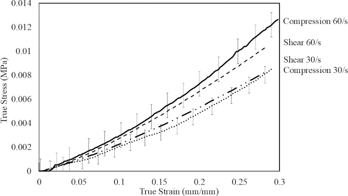
Figure 1: Brain tissue exhibits a similar mechanical response in compression and simple shear. True stress–strain curves are shown for uniaxial compression and simple shear at strain rates of 30 s⁻¹ and 60 s⁻¹. True stress-strain responses for compression and shear at both strain rates, demonstrating close agreement between loading modes. Please click here to view a larger version of this figure.

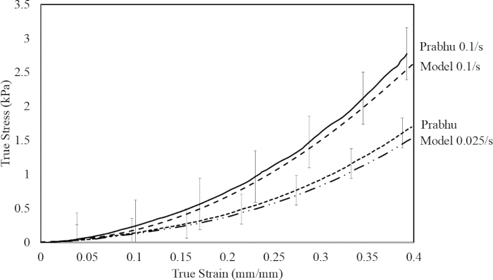
Figure 2: Model agreement with low-rate experimental brain tissue response. Experimental true stress–strain curves are compared with model predictions at strain rates of 0.025 s⁻¹ and 0.1 s⁻¹. The close agreement across both rates demonstrates that the model reproduces the low-rate compressive response³⁷. Experimental and model true stress–strain responses at 0.025 s⁻¹ and 0.1 s⁻¹. Please click here to view a larger version of this figure.

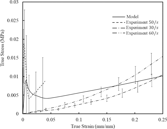
Figure 3: High-rate calibration of the brain ISV damage model using compression experiments. The updated brain damage Internal State Variable (ISV) model is compared with experimental true stress–strain responses in compression at high strain rates. Model response is shown alongside experimental curves at 30 s⁻¹, 50 s⁻¹, and 60 s⁻¹ to demonstrate agreement over the strain range used for calibration^38,39,28. Model prediction and experimental compression stress–strain curves at 30–60 s⁻¹. Please click here to view a larger version of this figure.

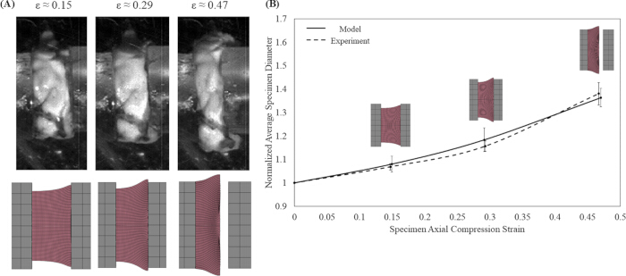
Figure 4: Comparison of FE simulation with SHPB experimental deformation and diameter evolution. Finite element (FE) predictions are compared with Split Hopkinson Pressure Bar (SHPB) experimental results to evaluate compressive deformation and lateral expansion during uniaxial loading. Agreement is assessed using specimen shape evolution at selected strain levels and the normalized diameter response over the full strain range. (A) Experimental specimen images and corresponding FE deformed shapes at axial strains ε ≈ 0.15, 0.29, and 0.47. (B) Normalized average specimen diameter versus axial compression strain, comparing model prediction with experimental measurements. Please click here to view a larger version of this figure.

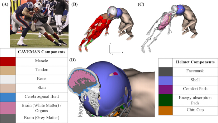
Figure 5: Field-to-simulation reconstruction and CAVEMAN model views for helmet-to-helmet impact. A representative helmet-to-helmet event is shown alongside the corresponding CAVEMAN full-body finite-element (FE) reconstruction used to generate solver-ready initial conditions. Model views highlight the global coordinate convention, whole-body posture alignment, and the head–helmet assembly with intracranial layers and helmet subcomponents.
(A) Field video frame showing helmet-to-helmet contact at the time of impact. (B) CAVEMAN full-body FE model at the reconstructed impact posture; axes indicate the global coordinate. system. (C) Skeleton-only view emphasizing player posture and alignment at impact. (D) Cutaway of the head–helmet assembly showing brain tissue (white/grey matter), cerebrospinal fluid (blue), and helmet components (shell, comfort pads, energy-absorption pads, facemask, chin cup). Please click here to view a larger version of this figure.

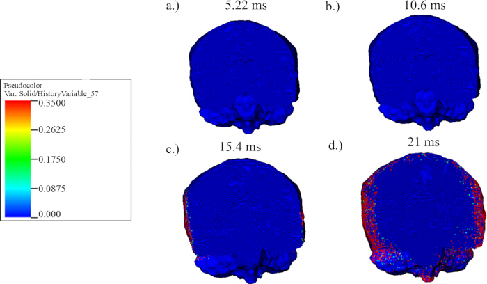
Figure 6: Temporal evolution of brain damage (HV57) in the 3D player-to-player impact simulation. Three-dimensional finite element (FE) results show the spatial progression of the HV57 brain damage metric over the impact event using the initial and boundary conditions defined in Table 1. Snapshots at four time points illustrate damage initiation and growth. (A) HV57 distribution at 5.2 ms. (B) HV57 distribution at 10.6 ms. (C) HV57 distribution at 15.4 ms. (D) HV57 distribution at 21.0 ms. Please click here to view a larger version of this figure.

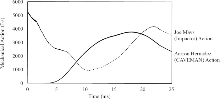
Figure 7: Mechanical action time histories for impactor and impacted head. Mechanical action (J·s) is plotted versus time for the impactor and the impacted (CAVEMAN) head during the reconstructed helmet-to-helmet collision. The curves summarize the temporal evolution of loading intensity and energy-transfer dynamics across the 0–25 ms impact window. Mechanical action histories for the impactor and impacted head, highlighting the crossover region associated with peak loading transfer. Please click here to view a larger version of this figure.

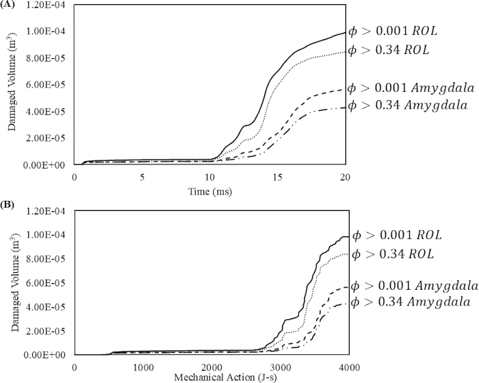
Figure 8: Damage-volume evolution versus time and mechanical action in a 9.3 m/s helmeted-head replay. Damage progression is quantified using the diagnostic damage variable, ϕ, reported as damaged volume in the right occipital lobe (ROL) and amygdala. Results are shown for two damage thresholds representing minimal (ϕ ≥ 0.001) and critical (ϕ ≥ 0.34) damage accumulation. (A) Damaged volume versus time for ROL and amygdala at ϕ ≥ 0.001 and ϕ ≥ 0.34. (B) Damaged volume versus mechanical action (J·s), indicating onset of rapid damage growth near ~2.8 × 10³ J·s.
Please click here to view a larger version of this figure.

Part	Material	Density, ρ (kg/m^3)	Elastic Modulus, E (MPa)	Poisson Ratio, ν	# of Elements, Ne	# of Nodes, Nn	Volume, V (m^3)	Mass, m (kg)
Impactor Foam	VN-600	97.5	5.84	N/A	25,746	5,161	4.43E-04	0.04
Impactor Cap	Nylon 66	1150	2930	0.37	14,874	3,411	1.10E-04	0.13
Facemask	Titanium (Ti64)	4430	113000	0.34	32,078	47,091	9.69E-05	0.43
Helmet Shell	Polycarbonate	1500	3356	0.4	376,335	92,738	1.06E-03	1.6
Helmet Foam	SM Firm	84.3	10.5	N/A	834,254	181,845	3.85E-03	0.32
Scalp	Scalp	1200	N/A	N/A	629,362	967,091	2.53E-03	3.04
Skull	Skull	1357	12040	0.22	308,554	498,436	9.43E-04	1.28
CSF	CSF	1040	0.3	0.5	124,603	209,893	2.60E-04	0.27
Brain	ISV	1000	N/A	N/A	185,858	276,691	1.19E-03	1.19

Table 1: Material properties, mesh discretization, and mass distribution of the helmeted-head finite-element model. The table summarizes the constituent materials, mesh characteristics, and component masses for the impactor, helmet, and anatomical structures used in the reconstructed helmet-to-helmet simulation. Reported quantities include density, p; elastic modulus, E; Poisson’s ratio, v; number of elements, N_e; number of nodes, N_n; component volume, V; and component mass, m. Abbreviations; CSF = cerebrospinal fluid; ISV = Internal State Variable material model; Ti64 = titanium alloy Ti-6Al-4 V; N/A indicates that the parameter was not applicable or was not prescribed as a constant material property for that component.

Metric	Median	IQR	95th Percentile	Acceptance Limit
Reprojection error (px)	2.7	2.4–3.1	3.6	≤ 8.0 px
Focal-length drift (%)	2.1	1.2–2.8	3	≤ 3.0 %
Landmark baseline drift (%)	2.3	1.5–3.1	5.2	≤ 6.0 %

Table 2: Reconstruction quality metrics for acceptance limits for the field-to-simulation workflow. Summary statistics are reported for the primary quality-control metrics used to evaluate video-based kinematic reconstruction, including reprojection pixel error (P_x), focal-length drift, and landmark baseline drift. Reported values include the median, interquartile range (IQR), 95th percentile, and the corresponding acceptance limit for each metric.

Item (units)	Real play (Reconstruction)	Applied to FE Players
Impacted v₀ (m/s)	[0.20, 8.3232, 0.00]	[0.20, 8.3232, 0.00]
Impacted ω₀ (rad/s)	[0.00, 0.00, 0.00]	[1.97, 45.01, 0.00]
Aaron Hernandez v₀ (m/s)	[0.00, 1.5234, 0.00]	[0.00, 0.00, 0.00]
Aaron Hernandez ω₀ (rad/s)	[2.00, 45.01, 0.00]	[0.00, 0.00, 0.00]

Table 3: Reconstruction-derived initial conditions at t_a and their application in the Finite Element (FE) model. The table compares the translational velocity, , and angular velocity, , obtained from the real-play reconstruction with the values applied in the finite-element (FE) model for Impactor and Impacted. Reported quantities are given as three-component vectors in the global coordinate system. For the CAVEMAN player, prescribed initial translational and rotational velocities were set to zero when whole-body motion and posture were carried directly by the reconstructed full-body model.

Quantity		Reconstruction peak	FE peak	Δpeak (%)	Δtpeak (ms)
		(value at time, ms)	(value at time, ms)
Linear accel (m/s2)		83.50 at 5.1	89.540 at 7.5	7.3	2.549285
Angular accel (rad/s²)		3153 at 5.2	3315.507 at 5.779	5.02	0.779902
Angular vel (rad/s)		45.01 at 15.0	59.95 at 13.909	24.9	1.090027

Table 4: Comparison of peak kinematic values from video reconstruction and Finite Element (FE) simulation during impact. The table compares peak linear acceleration, a, and angular acceleration, , and angular velocity, , obtained from the video-based reconstruction with the corresponding peak values from the finite-element (FE) replay. Reported values include the peak magnitude,Δ_peak, and time of occurrence, along with the percent difference in peak magnitude, , and the absolute difference in time-to-peak, Δt_peak

Supplementary Table 1: Equation for 6-DOF reconstruction. The table summarizes the equations used to map image-space landmarks to three-dimensional helmet motion, estimate translational and rotational kinematics, define the head center-of-gravity trajectory, smooth the reconstructed signals, and evaluate reconstruction quality. Reported terms include the projection model, intrinsic camera matrix, Universal Perspective-n-Point (UPnP)-based pose recovery, central-difference estimates of linear and angular motion, impact reference time, and reconstruction quality metrics. Root-Mean-Square Error (RMSE); Center of Gravity (CG); Pixels (P_x); Frames per Second (fps).Please click here to download this file.

Supplementary Table 2: Brain constitutive model. The table lists the constitutive, kinematic, flow-rule, hardening, and internal-variable evolution equations for amorphous glassy polymers, as human brain material. Equation numbers (A.1)—(A.27) correspond to the formulation implemented for brain tissue response in the present study.Please click here to download this file.

Supplementary Table 3: Constitutive parameters used in the calibrated brain damage material model. The table lists the calibrated parameter values used in the constitutive formulation, including elastic, strain-rate, yielding, hardening, internal strain, internal stress, and pore-growth terms.Please click here to download this file.

Discussion

This work couples single-view video–based 6-DOF reconstruction with full-body finite element (FE) replay to provide a process-only path from a real play to a numerically stable, configuration-faithful simulation. Unlike traditional laboratory tests (twin-wire drop standards; league laboratory linear-impactor tests), which deliberately idealize loading, the present workflow preserves event-specific conditions, helmet model and fit, player-to-player impact kinematics, and converts field footage into solver-ready boundary conditions. The intended outcome is not an injury verdict but a transparent replay that other laboratories can reproduce from the same inputs.

The procedure mirrors apparatus verification in classical high-rate testing. First, the helmet-only “shake” confirms that the FE surrogate is numerically ready (no negative volumes, bounded hourglass/contact energies, plausible strap loads). This step is a screen for run-ability, not a validation of helmet performance; the surrogate configuration has been used elsewhere^11,40,41,42. Second, video reconstruction quality checks set up geometric and temporal fidelity before any solver input is generated. Reprojection error, landmark baseline drift, and focal-length drift are reported with acceptance bands. These metrics quantify how closely the 3D solution is supported by the footage and field geometry. Third, driver fidelity (RMSE, | Δ_peak |, | Δ_tpeak | for linear and angular rates/accelerations) confirms that solver-applied motion matches the reconstructed target at the skull CG; without this check, tissue fields would be conditioned on an unknown input. A key modeling choice is to define t₀ at the peak | a | of the struck head and to apply velocities only to the impactor while leaving the impactee initially at rest. This prevents double-counting kinetic energy and preserves contact posture; it also isolates later dynamics to interactions among the helmet, head, neck, and bodies rather than imposed accelerations.

Unlike other calibration workflows, mechanical action is reported as the time integral of the kinetic energy (J·s) to quantify the duration – weighted accumulation of mechanical activity throughout the impact. Measures of mechanical action describe the evolution of mechanical activity throughout a medium and how it is transformed. Specifically, in this case, how the mechanical interaction between two players can be evaluated using dynamic energy exchange rather than kinetic prescriptions. The reconstructed replay reproduced physically consistent intracranial loading patterns (Figure 6). Time-stamped fields showed progressive nucleation, growth, and coalescence of the diagnostic damage variable ( φ ) over 5–21 ms, originating near high-tension and shear zones. These maps verify that the solver preserved the intended boundary-condition fidelity through realistic internal energy transfer.

Because broadcast footage lacks full camera calibration, the authors did not apply a lens distortion model. The principal point was assumed at the image center (c_x = 640,c_y = 360), and focal length was estimated per frame during pose recovery (zoom-aware UPnP). To suppress numerical noise from differentiation, linear and angular rates were filtered using a zero-phase moving-average method (15 Hz linear, 40 Hz angular; focal 5 Hz) and then differentiated to obtain accelerations.

Reconstruction accuracy varies with footage quality. Resolution, frame rate, compression, motion blur, and camera baseline each contribute. Low resolution and heavy compression increase digitization noise, inflating reprojection RMSE. Camera viewpoint changes, motion blur/occlusion, and zoom changes increase click noise and degrade pose recovery. Low frame rates (30 fps) limit temporal resolution and force larger derivative step sizes; this elevates and | Δt_peak | may under-resolve sharp angular pulses. Rolling shutters and interlacing can induce per-row time offsets; if suspected, tracking should be limited to near-central rows and panning segments avoided. For these reasons, the protocol reports QC with spread statistics (median, 95th percentile) and enforces hard cutoffs (0 frames > 8 p_x reprojection).

Cross-program reliability (NCAA programs) is defined here as independent groups reproducing the same solver-applied 6-DOF driver from the same video inputs and passing the same acceptance limits for reconstruction QC (Table 2) and driver fidelity (Table 4), after helmet readiness checks (no negative volumes; bounded hourglass/contact energies). The minimum reproducibility package is: (i) the digitized single-view landmark clicks kinovea_clicks.csv (frame, landmark, u, v), (ii) the 3D helmet landmark template helmet_landmarks.csv (m), (iii) Config.json and the reconstruction script reconstruct_6dof_upnp.py, (iv) exported outputs (poses_per_frame.csv, kinematics.csv, initial_conditions_t0.csv), and (v) QC summaries (qc_summary.txt, qc_per_frame.csv) plus solver versions and the run-deck entry point. Drop towers and linear impactors remain essential for comparative helmet assessment and certification. They provide repeatable measurements and are well-suited to ranking designs under standard pulses. They cannot, by design, capture multi-body coupling and off-axis contact, nor can they replay irregular time histories from specific collisions. The present field-to-simulation workflow complements those programs: it preserves event variability while codifying QC so that different groups, given the same video, can recover the same applied driver and compare how different helmets (or fits) behave in that event. So, reliability here means reproducible inputs and replay fidelity, not certification equivalence or injury determination. Moreover, replacing a physical ATD such as Hybrid III with a whole-body FE human (CAVEMAN) enables estimation of internal tissue fields using biofidelic, rate-sensitive constitutive laws and anatomically detailed geometry, thereby moving closer to actual human response under oblique, multi-planar loading^43,44,45,46. Hybrid III remains valuable for repeatable external kinematics and instrumentation, but its simplified neck and lack of deformable brain/soft-tissue representations limit inference of intracranial stress/strain. This distinction between style and instance is central: certification addresses style (standard pulses); reconstruction addresses the instance (the actual play) with human-relevant internal responses.

Mechanical-action histories for the impactor and impacted head (Figure 7) confirm consistent energy transfer within the reconstructed replay. The crossover of the two curves aligned with the interval of maximum intracranial stress and strain, showing that the applied kinematics produced a physically plausible exchange of momentum and mechanical activity through the coupled helmet–head–body system. The brain material was modeled using a physics-based Internal State Variable (ISV) formulation with a diagnostic scalar damage variable (Φ). In this implementation, Φ does not feed back into the stiffness but serves as an indicator of tensile-pressure- and shear-sensitive contributions to void nucleation. Here, “damage” refers to microscopic tearing within the cell walls of neurons and supporting tissues. Capturing these subtle, subcellular effects motivates the use of a physics-based framework such as the ISV model, which links observable macroscopic deformation to the underlying material response. Damage-volume analyses for the right occipital lobe and amygdala (Figure 8) showed a two-stage progression: early nucleation at 10–11 ms followed by a rapid rise near 15 ms. When plotted against mechanical action, both regions collapsed onto a single energetic threshold around 2.8 × 10³ J·s, suggesting a consistent trigger for rapid coalescence across tissue types. Because no experimental injury outcomes or subject-specific anatomy are incorporated, variables such as Φ, Head Injury Criterion (HIC), Severity Index (SI), and regional strain are reported solely as numerically consistent outputs of a reproduced kinematic history, not as validated predictors of injury. This distinction preserves the intent of the method: verifying numerical soundness, energy balance, and boundary condition fidelity while avoiding overinterpretation of biological injury mechanisms.

Finally, several limitations warrant acknowledgment. (1) Footage dependency: broadcast videos may be occluded, edited, or stabilized; any cut within the analysis window invalidates temporal coherence. (2) Full camera calibration was not performed. Lens distortion was not modeled; the principal point was assumed at the image center (c_x = 640,c_y = 360), and the focal length was estimated per frame. Reconstruction accuracy, therefore, depends on these assumptions, the quality of the digitized landmark clicks, and the accuracy of the 3D helmet landmark template (helmet_landmarks.csv). (3) Rigid coupling assumption: local shell or padding deformation may introduce minor deviations between helmet and skull motion. (4) Material generality: the CAVEMAN model and ISV constants stand for average human properties, not patient-specific variations, and thus microstructural injury mechanisms are not validated here. (5) Boundary completeness: neck muscle activation and pre-impact body motion are approximated through the t₀ velocity-seeding strategy, capturing the main collision exchange but omitting antecedent play dynamics.

This work sets up a transparent, reproducible field-to-simulation pipeline that translates broadcast video into solver-ready 6-DOF drivers and applies them to a configuration-faithful, helmeted whole-body FE model. By enforcing quality gates on helmet mass/CG agreement, mesh and contact stability, and target-vs-applied driver fidelity, the protocol certifies numerical readiness before any interpretation of internal player tissue-level response. The approach complements standardized lab tests by preserving event-specific hardware and kinematics (including faceguard and straps) while keeping injury inference out of scope; outputs serve as process diagnostics rather than verdicts. Practical limitations remain (video quality, similarity-scale assumptions, rigid landmark coupling, non-personalized anatomy, simplified pre-impact posture), but each is bound by reported metrics and mitigations. The immediate value is a proposed method for gathering real, unidealized kinematic data on dynamic player-to-player impact loading that other laboratories can replay to reproduce the same applied motion and compare alternative helmet configurations under the same real event. More broadly, the workflow generalizes beyond sport to crash and defense scenarios where ethical constraints prevent human testing, providing a consistent foundation on which future studies can add subject-specific anatomy, active musculature, or validated injury models without altering the reproducible core.

Materials

List of materials used in this article

Name	Company	Catalog Number	Comments
Video digitization software	Kinovea Project	N/A	Kinovea v2023.1.2 used to click helmet landmarks and export kinovea_clicks.csv (frame, landmark, u, v).
Reconstruction language/runtime	Python Software Foundation	N/A	Python v3.13.7 used to run the reconstruction script.
Computer vision library	OpenCV (opencv-python)	N/A	Required for cv2.solvePnPGeneric (UPnP) and Rodrigues rotation conversion.
Numerical computing libraries	NumPy; pandas	N/A	Used for vector/matrix ops, CSV I/O, and kinematic post-processing.
Reconstruction script	Custom (Supplementary)	reconstruct_6dof_upnp.py	Zoom-aware single-view UPnP pose per frame; outputs poses_per_frame.csv, kinematics.csv, initial_conditions_t0.csv, qc_summary.txt, qc_per_frame.csv.
Reconstruction configuration	Custom (Supplementary)	Config.json	Inputs: fps=59.94; principal_point=[640,360]; cutoffs (linear 15 Hz, angular 40 Hz, focal 5 Hz); helmet_to_com=[-0.1,0.4,0.0] m.
3D landmark template	Custom (Supplementary)	helmet_landmarks.csv	3D helmet landmark coordinates (m) in helmet coordinate system: (landmark, X, Y, Z).
Digitized landmark clicks	Custom (Supplementary)	kinovea_clicks.csv	Per-frame 2D clicks exported from Kinovea: (frame, landmark, u, v).
FE pre/post-processor	Livermore Software Technology Corporation (LSTC)	N/A	LS-PrePost v4.12 used to inspect meshes, mass properties, contacts, and apply/verify axes points P/Q if needed.
Veloldyne Explicit FE solver	Corvid Technologies	N/A	Velodyne explicit solver v24p11; used for replay simulations (hourglass, bulk viscosity, contact, mass scaling controls).
Full-body human FE model	Corvid Technologies	CAVEMAN v25p5 (licensed)	Finite-element human body model used for helmet coupling and whole-body replay; licensing may restrict redistribution.
2016 Riddell Revolution Speed Classic Helmet	Purdue University (Sean Bucherl); BioCore (source model)	BioCore RRSC v2 (Sep 2019); adapted Velodyne	2016 Riddell Revolution Speed Classic (RRSC) helmet FE surrogate used for coupling. Model provenance: based on the BioCore RRSC LS-DYNA model (v2 Sep 2019) and provided/adapted for this work by Sean Bucherl (Purdue University). Redistribution may be license-restricted; provide access upon reasonable request under the applicable agreement.