Reproducible Computational Workflow for Drug Discovery to Standardize Network Pharmacology and Molecular Docking Analyses

Summary

This standardized protocol unifies network pharmacology and molecular docking with Molecular Dynamics (MD) simulations for drug discovery. It establishes quantitative screening criteria and reproducible steps, suitable for multi-target drug screening using public datasets and improving result reliability.

Abstract

Network pharmacology and molecular docking are widely applied in drug discovery, yet fragmented workflows and inconsistent operations frequently undermine result reproducibility. Here, a standardized protocol integrating these approaches into a reproducible framework for drug screening and mechanism exploration is described, with the workflow organized into three sequential phases: data preparation, computational analysis, and validation. In the preparation phase, compound libraries from public databases are filtered via Absorption, Distribution, Metabolism, Excretion, and Toxicity (ADMET) criteria, including oral bioavailability, drug-likeness, and toxicity prediction, while potential therapeutic targets are obtained through target prediction and integration of disease-related databases to comprehensively identify drug-disease interaction candidates. In the computational analysis phase, overlapping targets undergo Gene Ontology (GO) and Kyoto Encyclopedia of Genes and Genomes (KEGG) enrichment analyses and protein-protein interaction network topological analysis to identify core targets; molecular docking is configured with two standardized optional strategies with distinct advantages. The two-step progressive strategy employs AutoDock Vina for high-throughput preliminary screening of the compound library, followed by precise re-docking with YASARA, which eliminates false positives from high-throughput screening and generates protein-ligand complexes natively compatible with subsequent YASARA molecular dynamics (MD) simulations to avoid structural deviations caused by cross-software format conversion. The one-step strategy completes the full docking process via YASARA alone, which simplifies the operation workflow, improves experimental efficiency, and is fully applicable for specific research goals. In the validation phase, standardized MD simulations evaluate ligand-protein complex stability via core metrics of root mean square deviation (RMSD) and root mean square fluctuation (RMSF). This unified, reproducible pipeline enhances the reliability of network pharmacology and docking studies and facilitates cross-study comparisons in computational drug discovery.

Introduction

Network pharmacology represents a research approach that deciphers the interaction patterns between drugs and the organism from a holistic network perspective¹. By constructing and analyzing the interaction network encompassing drug-component-target-disease-biological pathway, it quantitatively identifies the key molecules, core pathways, and synergistic mechanisms through which drugs exert their effects. This analytical framework aligns with the international standard for network pharmacology, which emphasizes multi-omics data integration and topological network analysis, and ultimately elucidates the overall therapeutic effects of drugs, predicts potential side effects, or provides systematic guidance for new drug development. Such a strategy has been successfully applied in diverse fields, including deciphering signaling pathways associated with target proteins of non-steroidal anti-inflammatory drugs (NSAIDs) against COVID-19, and exploring the mechanism of action of treating diseases like osteosarcoma and type 2 diabetes mellitus^2,3,4. This advantage drives the paradigm shift from single target to multi-target drug discovery in modern pharmacology.

Molecular docking is a computational simulation technique that employs algorithmic modelling to assess the spatial compatibility and interaction strength between small-molecule compounds and biological macromolecular targets, thereby predicting optimal binding configurations^5,6. Morris et al. introduced AutoDock4 and AutoDockTools4, which enable automated docking with selective receptor flexibility; these tools are based on molecular dynamics and molecular geometry, and evaluate binding stability and affinity by calculating energy differences between molecules⁷. Classic tools like AutoDock use semi-flexible ligand-receptor modelling and have become a gold standard for evaluating binding affinity in such simulations⁷.

In drug discovery, network pharmacology screening techniques are frequently employed to identify key components, which are then validated through molecular docking to assess their binding with target proteins, ultimately establishing the relationship between the drug and the disease⁸. However, current applications commonly suffer from inconsistent experimental design, non-standardized operational procedures, and missing validation steps. A systematic evaluation of herbal medicine-related network pharmacology studies has documented this widespread issue, noting that data heterogeneity across databases and inadequate experimental validation lead to irreproducible results⁹. These limitations not only undermine the reproducibility and reliability of research outcomes but also hinder the translation of computational predictions into experimental validation. Unlike isolated network pharmacology studies that lack experimental validation or fragmented docking workflows with arbitrary parameters, this protocol integrates both approaches with standardized thresholds and step-by-step operations. This framework eliminates subjective parameter selection, ensuring the workflow can be replicated by different operators with consistent results.

Therefore, establishing standardized operational procedures to identify potential drug targets and pathways through network pharmacology screening, combined with molecular docking to validate drug-target binding activity, can provide experimental evidence for studying drug mechanisms of action and screening candidate drugs¹⁰. This protocol is particularly suitable for multi-target drug screening of drug components and synthetic small molecules using publicly available omics, chemical, and protein structure databases; it is not applicable to targets without resolved crystal structures, or single-target orphan drug screening with no known disease-related interaction networks.

Protocol

This protocol involves only computational analyses of publicly available databases and does not involve the use of human subjects, vertebrate animals, or biological tissues. All the summary workflows described in this section are illustrated in Figure 1.

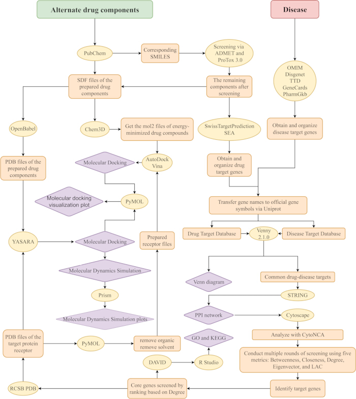
Figure 1: Summary of the workflow. Green rectangles represent alternative drug components, red rectangles represent diseases, yellow ellipses contain the websites and software used, orange rectangles contain the obtained files or data, as well as key steps, and purple diamonds represent the final required results. Please click here to view a larger version of this figure.

1. Acquisition of drug components and targets

1. Search the PubChem database (https://pubchem.ncbi.nlm.nih.gov/) using chemical names as keywords to obtain the corresponding SMILES (Simplified Molecular-Input Line-Entry System) strings.
2. Access the ADMETlab 3.0 website (https://admetlab3.scbdd.com/), select the ADMET Evaluation option under the Services tab, input the SMILES strings, and click the SUBMIT button.
3. Filter the ADMET results based on indicators: Absorption, Distribution, Metabolism, Excretion, Toxicity, Medicinal Chemistry, and Toxicophore Rules. Retain only compounds that meet all pre-defined threshold criteria for each indicator (Table 1).
4. Access the ProTox 3.0 website (https://tox.charite.de/protox3/index.php?site=home), input the SMILES strings of the compounds filtered, select the TOX PREDICTION module, tick all desired prediction options (e.g., organ toxicity, carcinogenicity), and run the prediction.
5. Screen out compounds with predicted toxicities that exceed pre-defined safety thresholds based on the ProTox 3.0 results (Table 2).
6. Compile the compounds that pass both ADMET and ProTox 3.0 screening into a structured drug-component database (e.g., Excel or CSV format) with columns for compound name, SMILES, and screening status.
7. Access the SwissTargetPrediction website (https://swisstargetprediction.ch/), select Homo sapiens from the organism dropdown menu, input the SMILES strings of the components in the drug-component database, click the Predict targets button, and collect all predicted targets with a Probability score greater than 0.
8. Access the SEA (Similarity Ensemble Approach) website (https://sea.bkslab.org/) and input the same SMILES strings used above for target prediction and filter the results to retain only entries in the Target Key field that end with _Human and have a p-value below 0.05.
9. Combine the target lists obtained from SwissTargetPrediction and SEA into a single drug-action target library. Remove duplicate targets and standardize target names to official gene symbols (e.g., using HGNC guidelines) via Uniprot (https://www.uniprot.org/).
   NOTE: The drug-action target library can be saved as a CSV file for later use.

Table 1: ADMETlab 3.0 threshold criteria for drug safety screening. The table summarizes the recommended cutoff values and classification ranges for key physicochemical properties, ADME parameters, metabolism interactions, toxicity endpoints, toxicity pathways, and toxicophore rules. Predictions are categorized into three risk levels (low, medium, and high) based on probability values (< 0.3, 0.3 - 0.7, > 0.7) or quantitative ranges, enabling systematic evaluation of compound safety profiles during early drug discovery. Please click here to download this Table.

Table 2: ProTox-3.0 threshold criteria for toxicity prediction in drug discovery. The table summarizes key toxicity endpoints predicted by ProTox 3.0, with a focus on parameters critical for drug safety assessment during early drug discovery. Each endpoint returns a binary classification (Active or Inactive) accompanied by a probability score (0-1), where Active indicates potential toxicity risk. Priority should be given to organ toxicities (hepatotoxicity, cardiotoxicity), toxicity endpoints (carcinogenicity, mutagenicity, immunotoxicity), and CYP metabolism inhibition, as these are major causes of clinical attrition. Multiple active hits across endpoints suggest broad toxicity potential and warrant compound deprioritization. Acute toxicity is assessed via predicted LD50 and GHS class, with Class 1 - 3 (< 300 mg/kg) considered highly toxic. Probability scores provide confidence levels for each prediction. Please click here to download this Table.

2. Acquisition of disease targets

NOTE: When screening databases, standardize target gene naming conventions to prevent omissions caused by nomenclature discrepancies.

1. Access five disease-related databases: OMIM (https://www.omim.org/), Disgenet (https://disgenet.com/), TTD (https://ttd.idrblab.cn/), GeneCards (https://www.genecards.org/), and PharmGkb (https://www.pharmgkb.org/). Apply the following database-specific screening criteria: for GeneCards, filter entries with a Relevance score ≥ 1.0; for DisGeNET, select entries associated with the target disease; for PharmGKB, restrict results to gene-related entries by selecting the Gene option; for TTD, retain entries where the Disease column matches the target disease.
2. For each database, use the official name of the target disease (e.g., Alzheimer’s disease) as the search keyword to retrieve all associated targets.
3. Collate the target lists from all five databases into a single spreadsheet. Remove duplicate targets by comparing gene symbols across lists.
4. Standardize all remaining target names to official gene symbols via Uniprot to resolve nomenclature inconsistencies. Save the standardized, deduplicated list as a disease target library (CSV or Excel format).
   NOTE: The disease target library can be saved alongside the drug-action target library (Step 1.9) for later use in Step 3.

3. Acquisition of common drug-disease targets

1. Access the Venny 2.1.0 web tool (https://bioinfogp.cnb.csic.es/tools/venny/). Import the drug-action target library (Step 1.9) and disease target library (Step 2.4) into the two input fields of Venny 2.1.0 to create a Venn diagram showing the overlap between the two target sets.
2. Extract the intersection targets from the Venn diagram results. Label these as common drug-disease targets (potential interaction points) and save them as a CSV file.

4. Construction of protein-protein interaction (PPI) networks and core target analysis

1. Access the STRING database (https://cn.string-db.org/). Select Homo sapiens as the Organism from the dropdown menu.
2. Import the common drug-disease targets (Step 3.2) into the STRING input field. Set the minimum required interaction score parameter to high confidence (0.700) and click Search to generate PPI data. Export the PPI data as a TSV (tab-separated values) file.
3. Open Cytoscape software with the CytoNCA plugin pre-installed. Import the PPI TSV file into Cytoscape using the File > Import > Network from File menu.
4. Launch the CytoNCA plugin by clicking Apps > CytoNCA > Open. Select five reference metrics for core target screening: Betweenness, Closeness, Degree, Eigenvector, and LAC.
   NOTE: Five key topological metrics used are namely Betweenness (betweenness centrality, measuring the frequency of a target appearing on all shortest paths in the network), Closeness (closeness centrality, reflecting the average shortest path length from a target to all other targets in the network), Degree (local connection degree, quantifying the number of direct interactions between a target and other targets), Eigenvector (eigenvector centrality, weighting both the target’s own connectivity and the importance of its connected targets), and LAC (local average connectivity, assessing the connection density among the direct neighboring nodes of a target).
5. Launch network analysis by clicking Tools > Analyze Network menu, then click OK. Export the analysis results into a CSV table.
6. Calculate the median value for all five metrics and retain targets that meet or exceed the median. Repeat Step 4.5 multiple times until 10 to 20 targets remain.
7. Rank the remaining targets by the Degree metric (highest to lowest) and preliminarily select the top 10 targets as core genes. Save the core gene list as a CSV file.
   1. To reduce false positives and ensure that only structurally suitable targets proceed to docking, perform further evaluation for structural feasibility and druggability: check the PDB database for available high resolution crystal structures (≤ 2.5 Å) or assess whether a reliable homology model can be constructed; use pocket prediction tools to confirm the presence of suitable binding sites; and cross reference with literature or functional databases to verify documented relevance to the disease pathway.
   2. Deprioritize targets that lack structural availability, druggable pockets, or disease relevance for docking studies. GO and KEGG enrichment analysis can still be performed using the full core target list from this step, as it does not require structural information.
      NOTE: The number of genes in Steps 4.6 and 4.7 can be changed as needed. Typically, 10 to 20 targets remain after Step 4.6, and maintaining at least 10 core genes in Step 4.7 is recommended to ensure sufficient data volume for reliable GO and KEGG enrichment analysis and consistent visualization trends.

5. GO and KEGG enrichment analysis and visualization

NOTE: This part clarifies gene functions at the cellular component, functional, and intracellular pathway levels.

1. Access the DAVID web tool (https://davidbioinformatics.nih.gov/home.jsp). Select Gene List as the input type and import the core genes into the input field.
2. Set the Identifier to OFFICIAL_GENE_SYMBOL and select Homo sapiens in Select species. Then, click Submit List to upload the core genes.
3. For GO enrichment analysis, select the GOTERM_BP_DIRECT, GOTERM_CC_DIRECT, and GOTERM_MF_DIRECT categories.
4. For KEGG enrichment analysis, select the KEGG_PATHWAY category. Set the significance threshold to p < 0.05 for both GO and KEGG analyses.
5. Click the Functional Annotation Chart to generate enrichment results. Export the GO and KEGG results as CSV files. Use R Studio software with ggplot2 to create bar charts or bubble plots for the top 10 enriched terms/pathways.
   NOTE: The number of displayed terms/pathways can be adjusted according to requirements.

6. Molecular docking using Autodock Vina

NOTE: Step 6 and Step 7 are both molecular docking steps. Step 6 uses AutoDock Vina 1.1.2 software, while Step 7 uses YASARA 10.3.16. Using YASARA facilitates the subsequent YASARA molecular dynamics simulation. If the docking results from AutoDock Vina are required, the docking results in YASARA should be consistent with those from AutoDock Vina. This avoids discrepancies caused by software switching and also ensures the reliability of the molecular dynamics simulation validation results, with detailed method: Open the "result.pdb" result of Step 6.31 using LigPlot+ (Version 2.3) to generate a 2D interaction diagram, identify the key residues interacting with the ligand, then select the key residues in the docking step 7.18 of YASARA, and set the box size to cover the binding pocket, so as to maximize the consistency of the docking sites between Vina and YASARA. Subsequently, when selecting the optimal docking results in Step 7.19, ensure that the key interacting residues between the ligand and receptor remain consistent with those identified from the AutoDock Vina results. This consistency requirement focuses on the preservation of essential interaction patterns rather than exact atomic correspondence; minor variations in peripheral residue conformations are expected due to differences in force field parametrization and side chain flexibility. As long as the critical interactions with key active‑site residues are conserved, the docking results can be considered consistent for cross‑validation purposes. If AutoDock Vina docking (Step 6) is not required, Step 7 can be performed directly.

1. Obtain the SDF (Structure Data File) of the drug compounds named ligand.sdf from the PubChem database by searching for the corresponding SMILES strings (Step 1.1).
2. Open SDF files using Chem3D software. Under the Calculation option, select MM2 and click Minimize Energy to perform free energy minimization of the compound structure.
3. Save the minimized structure as a ligand.mol2 file by selection File > Save As. Obtain the PDB (Protein Data Bank) format file of the core gene’s protein receptor from the RCSB PDB database (https://www.rcsb.org/; search by PDB ID or gene name) named receptor.pdb.
   1. Prioritize structures with a resolution ≤ 2.5 Å and resolved binding sites if available. When selecting a structure, examine the entry for completeness (e.g., presence of all expected domains, absence of large unresolved loops), potential mutations that could affect ligand binding, and whether functionally important cofactors (e.g., heme, metal ions) or co-crystallized ligands are included.
   2. For targets with known oligomeric assemblies, consider whether the monomeric or multimeric form is appropriate for the research question; the biological assembly can be downloaded if dimeric or higher-order interactions are relevant. The chosen structure will undergo further preparation in subsequent steps, so initial inspection helps avoid downstream complications.
4. Open the receptor.pdb using PyMOL software. Type remove organic in the command line and press Enter to eliminate small-molecule ligands from the protein structure.
   NOTE: If using the co-crystallized ligand to define the binding site, first record the 3D center coordinates of the ligand, then type remove organic in the PyMOL command line and press Enter to delete co-crystallized small molecules; otherwise, directly run the remove organic command to remove co-crystallized small molecules.
5. Type remove solvent in the command line and press Enter to remove free water molecules from the protein structure; use the command select metal_cofactor, resn [target cofactor residue name] to identify functionally critical metal ions or cofactors (e.g., HEM, Zn²⁺, Mg²⁺) and confirm their retention in the structure.
6. Export the cleaned receptor from PyMOL as receptor_clean.pdb by clicking File > Export Molecule > Save.
7. Open receptor_clean.pdb in UCSF Chimera 1.19. Display the sequence by clicking Tools > Sequence > Sequence to inspect for missing loops adjacent to the binding site (missing regions are indicated by red outline boxes). If missing loops are present, rebuild them by selecting Structure > Modeller (loops/refinement) from the sequence window menu, choosing non-terminal missing structure, setting an appropriate number of models (e.g., 5), and proceeding with the calculation. After completion, select the most reasonable model.
8. Optimize the structure in Chimera. Use the Rotamers tool (Dunbrack library) on selected residues to optimize side chains, adding Clashes and H‑Bonds via the Columns menu for evaluation and selecting conformations with minimal clashes (0 - 1 preferred) and favorable H‑bonds. Then add hydrogen and assign charges using Dock Prep (AMBER ff14SB). Finally, perform energy minimization with the Minimize Structure tool, fixing backbone atoms by selecting them (sel @ca,c,n,o), inverting the selection, and enabling Fixed atoms. Save the processed structure as receptor_optimized.pdb by selecting File > Save PDB.
   NOTE: Skip side chain optimization for well‑ordered residues. Dock Prep automatically handles protonation. Minimization should be performed with the backbone fixed.
9. Reopen receptor_optimized.pdb in PyMOL and define the canonical binding site. If a co-crystallized ligand is present, use its coordinates to center the grid: record the ligand's center, then remove it with remove organic. If no co-crystallized ligand is available, define the binding site based on known key residues from literature (e.g., select binding_site, resi XXX-XXX) or by visually identifying the putative binding pocket using pocket prediction tools to validate the visual assessment. Record the 3D center coordinates (x/y/z) of the defined site for grid box setup.
   NOTE: The coordinates recorded here are used to center the AutoDock Vina grid. For a residue-based definition, the geometric center of the selected residues should be calculated; for a pocket identified visually or by prediction tools, the center of the cavity is employed. When defining the binding site, consideration must be given to whether the intended docking strategy targets the orthosteric (active) site or an allosteric site. For orthosteric targeting, the binding site should be defined based on a co-crystallized ligand or conserved active-site residues reported in the literature. For allosteric targeting, pocket prediction tools may be employed to identify potential allosteric sites, particularly for targets with known allosteric regulations. In the absence of prior information, global docking followed by clustering of predicted binding hotspots can assist in identifying potential allosteric sites. This flexibility enables the protocol to accommodate both orthosteric and allosteric drug discovery campaigns.
10. Export the final optimized structure from PyMOL as receptor.pdb by clicking File > Export Molecule > Save.
11. Open receptor.pdb in AutoDock Tools 4.2.6 by clicking File > Read Molecule. Define flexible residues. Click Edit > Flexible Residues > Select Residues and choose binding site residues expected to undergo conformational changes upon ligand binding (select ≤ 10 residues).
    NOTE: This step allows selected side chains to move during docking, accounting for induced fit effects.
12. Save the receptor with flexible residues as a PDB file. Click File > Save, select Write PDB from the dropdown menu. In the Available PDB records window, tick ATOM and CONECT, click ADD, then click OK. Save the file as receptor.pdb.
    NOTE: This PDB file contains information about flexible residues and will be used to generate the PDBQT file.
13. Prepare the macromolecule for docking. Click Grid > Macromolecule > Choose, select the receptor.pdb file, and click Select Molecule. Save the receptor as a PDBQT file by clicking File > Save As and name it receptor.pdbqt.
    NOTE: AutoDock Tools assigns charges and atom types, saving the receptor in AutoDock's native PDBQT format, ready for grid box generation and docking calculations.
14. Click the Ligand menu, select Input, then click Open. Select ligand.mol2 and click OK. Click the Ligand menu, select Torsions, then click Detect Torsions. AutoDock Tools will automatically identify rotatable bonds in the ligand structure (e.g., single bonds in alkyl chains, amide bonds excluding peptide bonds).
15. In the Torsion Selection window, verify the detected rotatable bonds (retain all valid rotatable bonds, exclude rigid bonds such as aromatic ring bonds). Click Set to confirm the torsion definitions, then click Close.
    NOTE: Retaining valid rotatable bonds ensures the ligand can adopt different conformations during docking (flexible ligand), while keeping the receptor rigid — this is the core of semi-flexible docking in AutoDock Vina.
16. Click Ligand menu again, select Output, then click Save as PDBQT. Name the file ligand.pdbqt and save it in the same directory as receptor.pdbqt.
17. Click the Display menu, select Secondary Structure. Click Display Only, then select Lines and click Undisplay to simplify the protein view.
18. Click the Grid menu, select Grid Box. Adjust the x, y, z (center coordinates) and Spacing(Å) values to position the box over the protein’s active site.
    NOTE: If the binding site is unknown, use pocket prediction tools (e.g., CASTp, DoGSite) to identify putative binding pockets. Covering the entire protein significantly increases false positives and computational cost and is not recommended.
19. Click File > Close saving current, then click Grid > Output > Save GPF to save the grid box settings as Grid.gpf.
20. Open Grid.gpf with a text editor and record the gridcentre (x, y, z values) and npts (size x, y, z values) from the file.
21. Create a new text file named Config.txt and type the following content:
    receptor = receptor.pdbqt
    ligand = ligand.pdbqt
    center_x = [gridcentre x value from Grid.gpf]
    center_y = [gridcentre y value from Grid.gpf]
    center_z = [gridcentre z value from Grid.gpf]
    size_x = [npts x value from Grid.gpf]
    size_y = [npts y value from Grid.gpf]
    size_z = [npts z value from Grid.gpf]
    energy_range = 5
    num_modes = 10
    Replace the bracketed text with values from Grid.gpf (Step 6.19).
    NOTE: The energy_range parameter should be set as the maximum allowable energy difference relative to the optimal combined model, with units in kcal/mol. For example, setting it to 5 means that AutoDock Vina will terminate calculations once the energy difference from the optimal model reaches 5 kcal/mol. Additionally, num_modes specifies the number of binding models to generate, which is typically set to 10.
22. Place the vina_split.exe and vina.exe files in the same directory as receptor.pdbqt, ligand.pdbqt, and Config.txt.
23. Open the Windows System Console, navigate to the directory using the cd command (e.g., cd C:\DockingFiles).
24. Type the following command and press Enter: vina.exe --config config.txt --log log.txt --out output.pdbqt
25. Wait for the docking to be completed (duration varies by system). Two files will appear: log.txt (docking results) and output.pdbqt (lowest energy ligand structure). To ensure reproducibility, three independent docking runs are performed with different random seeds. An RMSD < 1.0 Å among the top poses confirms consistency.
    NOTE: As an empirical reference, AutoDock Vina binding energies (kcal/mol) can be interpreted as: ≤ -7 (high affinity, potential active conformations), -7 to -5 (moderate affinity), ≥ -5 (low affinity). These thresholds are system-dependent and should be validated with experimental data.
    1. To assess docking accuracy and discrimination capability for a specific target, two complementary validation approaches are recommended. Use redocking validation using crystallographic ligands to evaluate whether the protocol can reproduce experimentally observed binding modes, with RMSD < 2.0 Å serving as the standard acceptance criterion.
    2. Use enrichment analysis using public benchmark datasets (e.g., DUD-E) to assess the protocol's ability to distinguish true active compounds from property-matched decoys; this involves calculation of ROC curves (providing a global measure of classification performance) and enrichment factors such as EF1% (quantifying the enrichment of actives in the top-ranked fraction). Together, these validation steps help establish appropriate affinity cutoffs and ensure reliable screening performance for the target class of interest.
26. Open PyMOL software. Import output.pdbqt and receptor.pdbqt by clicking File > Open. Save the combined structure as result.pdb by clicking File > Save As.
27. Clear the PyMOL workspace by clicking File > New Session, then re-open result.pdb to visualize the ligand-protein complex.

7. Molecular docking using YASARA

NOTE: This step serves as the precise re-docking and pre-processing for subsequent molecular dynamics (MD) simulation and is a progressive verification of the high-throughput preliminary screening results from Step 6. Step 6 uses AutoDock Vina, the gold-standard tool for high-throughput virtual screening, to rapidly screen candidate molecules with excellent binding affinity from the compound library. This step adopts YASARA for docking, as its docking module is fully compatible with the YASARA MD simulation platform, which can avoid structural deviations caused by file format conversion and software switching, and provide a standardized initial complex structure for subsequent MD simulation. For all candidate molecules screened by AutoDock Vina in Step 6, the docking results (including binding pose in the active pocket and key amino acid interactions) obtained in this step must be consistent with those from AutoDock Vina, and the relative ranking of binding affinity must keep the same trend before proceeding to MD simulation. The absolute docking scores are not directly comparable between the two software due to different calculation algorithms. This consistency requirement can eliminate false positive results caused by software differences, ensure the stability of the binding characteristics of candidate molecules, and guarantee the reliability and logical continuity of subsequent MD simulation validation.

1. Utilize OpenBabel to convert the ligand.sdf file into the ligand.pdb file.
   NOTE: OpenBabel is used here only for format conversion. The actual parameterization of the ligand for molecular dynamics will be performed automatically by YASARA in subsequent steps.
2. Open YASARA software. Click File > Load and select ligand.pdb to import the ligand. Click Edit > Clean > All to remove structural defects from the ligand.
   NOTE: This step performs basic geometry cleanup. YASARA will then automatically assign force field parameters to the ligand using its built‑in AutoSMILES technology, which applies the General AMBER Force Field (GAFF) and AM1‑BCC charges to ensure compatibility with the AMBER14 force field used for the protein. This parameterization is essential for accurate energy calculations in both docking and MD simulations.
3. Click Options > Default pH, select the appropriate pH (e.g., 7.4 for physiological conditions), and click OK.
4. Click Dock > Force field to set the docking force field, ensuring parameter consistency with subsequent MD simulations.
   NOTE: AMBER14 is the recommended force field for this drug discovery workflow in YASARA 10.3.16, as it provides comprehensive parameter coverage for proteins and is fully compatible with standard MD simulation protocols. For standard protein residues, parameters are automatically assigned from the force field's built‑in templates. For small‑molecule ligands, YASARA automatically performs parameterization using its built‑in AutoSMILES technology, which assigns GAFF (General AMBER Force Field) atom types and AM1‑BCC charges. This ensures compatibility between protein and ligand parameters, enabling accurate energy calculations in both docking and MD simulations. A more appropriate force field may be selected according to the actual YASARA version used and the specific characteristics of the system.
5. Click Simulator > Define simulation cell > around all atoms to set the working boundary. Click Simulator > Cell boundaries > Periodic to enable periodic boundary conditions.
6. Click Options > Choose experiment > Energy minimization, then click Run to minimize the ligand’s energy.
7. Click File > Save as, name the file ligand.pdb, and click OK to overwrite the original ligand PDB file. Click File > New to clear the workspace, then click File > Load and select the receptor.pdb file.
8. Repeat steps 7.2 to 7.7 for the protein receptor, saving the processed file as a new receptor.pdb file.
9. Click File > New, then click File > Load and select both ligand.pdb and receptor.pdb. Repeat steps 7.3 to 7.5 to set pH, define the simulation cell, and enable periodic boundaries for the complex.
10. Click Processors > Set CPU and select the number of CPU cores to use. Click Processors > Set GPU and select the GPU device to accelerate computations.
11. Click File > Save as > YASARA Scene, name the file sce\nesult.sce (create the sce folder if it does not exist), and click OK.
12. Click Options > Macro&Movie > Set target, select sce\nesult.sce, and click OK. Click Options > Macro&Movie > Play macro, select the dock_run.mcr macro file, and click OK.
13. Click Simulator > Define simulation cell > around selected atoms and repeat 7.5, then click Continue to start the docking.
14. Wait for docking completion. Files with the yob suffix will be generated; name.log contains the binding energy and Contacting Receptor Residues.
    NOTE: To ensure the rationality of molecular dynamics simulation validation, select the docking result in YASARA that is consistent with the docking result of AutoDock Vina.

8. Molecular dynamics simulation

1. Click File > New to clear the workspace. Then click File > Load > YASARA Object and select result.yob.
2. In the SCENE CONTENT panel (right side), expand all Mol entries. Click Edit > Split > Object, select all Mol contents in the Sequence panel, and click OK.
3. Click Edit > Join > Object, select all Mol contents except the first and last entries (ligand), and click OK. Select the first Mol entry and click OK again to rejoin the protein.
4. Proceed to renumber the components. Select Renumber under Edit and click Objects. This generates two parts: the first part is the protein-receptor complex, and the second part is the small-molecule ligand.
5. Click Edit > Transfer, then click the Object option from the dropdown list. In the Sequence panel, first select the small-molecule ligand content by clicking its corresponding entry. Then select the protein receptor content by clicking its entry and click OK to confirm the selection pair.
6. In the next pop-up window, check the option starting with Fix atoms on screen during the transfer, and click OK.
7. Repeat Steps 7.2 to 7.5, then click Simulator > Temperature and select 298K. Click File > Save as > YASARA Scene, name the file sce\nesultrun.sce, and click OK.
8. Click File > New to clear the workspace. Then click Options > Macro&Movie > Set target, select sce\nesultrun.sce, and click OK.
9. Ensure that the force field selected in Step 7.4 is also used for the MD simulation; the md_run.mcr macro typically inherits the current force field settings. Click Options > Macro&Movie > Play macro, select the md_run.mcr macro file, and click OK to start the Molecular Dynamics Simulation.
10. Perform three independent MD simulations (3 x 100 ns) with different initial velocities for the protein-ligand complex and conduct statistical analysis of the three trajectories to ensure the reliability of the results. During the operation, files in the sim format will be generated. For example, if the trajectory is saved every 100 ps, a 100 ns simulation will generate 1000 files with the sim suffix.
11. Once Step 8.10 is complete, click Options > Macro&Movie > Set target, select the sce\nesultrun.sce file, and click OK.
12. Click Options > Macro&Movie > Play macro, select md_analyze.mcr, md_analyzebindenergy.mcr, and md_analyzeres.mcr and click OK.
13. After all three analyses are complete, the corresponding data files result_run_analysis.tab, result_run_bindenergy.tab, and result_run_analysisres.tab will be generated.
14. First, analyze result_run_analysis.tab, which provides 10 core parameters: Energy (total system energy), Bond (bond energy), Angle (bond angle energy), Dihedral (dihedral angle energy), Planarity (planarity energy), Coulomb (electrostatic energy), VdW (van der Waals energy), CA (Cα RMSD of the protein RMSD), Backbone (protein backbone RMSD), and HeavyAtoms (heavy atom RMSD).
15. Extract the Time (ns) column and corresponding parameter columns to assess whether the system reaches energetic equilibrium. Confirm system stability by the stabilization of potential energy within a narrow fluctuation range after the initial 10 - 20 ns. Evaluate conformational stability by monitoring the root-mean-square deviation (RMSD) of Cα atoms, protein backbone, and heavy atoms. The simulation was deemed structurally stable once these RMSD values reached a plateau.
16. As empirical reference points for protein–ligand complexes of typical size, Cα and backbone RMSD values plateauing below 2.5 Å, together with heavy‑atom RMSD below 3.5 Å, can be considered supportive indicators of conformational stability. Critically, use the primary and mandatory criterion and the presence of a clear plateau phase in the RMSD trajectory, rather than strict adherence to these numerical values alone.
    NOTE: These threshold values are empirical and should be interpreted in the context of the specific protein size and flexibility. The decisive indicator of convergence is a sustained plateau, indicating that the structure has stabilized around a consistent conformational ensemble.
17. Next, analyze result_run_bindenergy.tab, which provides the binding energy between the ligand and target over the simulation trajectory. Calculate the average binding energy across the entire simulation period. In YASARA's MM‑PBSA implementation, more positive values indicate stronger binding. A moderately strong and stable interaction is typically indicated by a mean binding energy that is positive and sufficiently large (the specific numerical value is system‑dependent but can be calibrated against known binders or experimental data), together with a standard deviation that is small relative to the mean (e.g., coefficient of variation < 50 - 60%), reflecting limited fluctuation during the simulation.
    NOTE: The binding energy reported in this step is calculated using the rigorous MM‑PBSA method, in contrast to the default YASARA binding energy macro which employs a faster approximation (BoundaryFast). The default approximation is suitable for rapid screening or relative comparisons, while the MM‑PBSA method is recommended for obtaining more accurate absolute binding free energies. As explicitly stated by the author in the YASARA macro header: More positive energies indicate better binding, negative energies DO NOT indicate no binding. Therefore, users should interpret positive values as indicative of stronger binding, with the numerical magnitude depending on the specific protein‑ligand system.
18. Finally, analyze the file result_run_analysisres.tab, which provides per-residue data including Residue ID, RMSD, Backbone RMSD, HeavyAtoms RMSD, and RMSF. Focus the analysis on the stable production phase identified. First, identify residues within the target's active site (e.g., those within 5 Å of the ligand). Then, use the data to assess the conformational stability of these individual active-site residues during the simulation.
    NOTE: As empirical reference points for stable active-site residues in protein-ligand complexes, RMSF values below 1.0 Å and RMSD fluctuations within 1 - 1.5 Å during the stable phase are generally considered indicative of well-maintained local conformations. Residues with RMSF exceeding 2.0 Å may indicate greater flexibility; such residues should be mapped onto the three-dimensional structure to determine if they correspond to functionally relevant flexible regions (e.g., loops or surface areas) or indicate potential instability within the binding pocket. These numerical guidelines are not absolute rules; the primary criterion is the absence of large conformational drift, which should be assessed in conjunction with the overall system convergence established.
19. Once data files are organized, import the organized data into Prism to generate corresponding plots.

Results

Following the network pharmacology analysis of loratadine against allergic rhinitis (AR), the interaction between loratadine and PTGS2 was selected as a representative case study to illustrate the step‑by‑step application of the molecular docking and MD simulation protocol. This example is intended to demonstrate workflow execution and data interpretation, rather than to provide biological validation of the specific interaction. For quantitative assessment against experimental data, users are encouraged to apply the prot...

Discussion

Significance and critical steps
This protocol combines network pharmacology, molecular docking, and molecular dynamics simulation, which offers distinct advantages over standalone methods or dual-combination workflows, and can help address key inefficiencies and reliability gaps in current drug discovery. The entire process relies on three critical steps that ensure its reliability, each addressing a core challenge in computational drug screening. First, multi-database integration (e.g., PubChem fo...

Materials

List of materials used in this article

Name	Company	Catalog Number	Comments
ADMETlab 3.0	Shanghai Institute of Materia Medica (SIMM), Chinese Academy of Sciences	N/A	Online platform for ADMET (Absorption, Distribution, Metabolism, Excretion, Toxicity) property prediction; used for evaluating the pharmacokinetic and toxicological profiles of ligands (URL: https://admetlab3.scbdd.com/)
AutoDock Tools (AutoDock 4)	The Scripps Research Institute	AutoDock 4.2.6	Software suite for molecular docking simulations; includes AutoDock 4 for docking and AutoDockTools (ADT) for preparing protein and ligand input files (adding hydrogens, assigning charges, setting rotatable bonds), defining docking grids, and analyzing docking results.
AutoDock Vina	The Scripps Research Institute	AutoDock Vina 1.1.2	Open-source molecular docking software; used for predicting binding affinities and poses between small-molecule ligands and protein receptors
Chem3D	PerkinElmer Informatics	Chem3D 2024	Molecular modeling software; used for constructing, optimizing, and visualizing 3D structures of small-molecule ligands
Cytoscape	Cytoscape Consortium (Institute for Systems Biology)	Cytoscape 3.10.3	Open-source software for visualizing and analyzing biological networks; used for constructing and editing gene/protein interaction networks
DAVID (Database for Annotation, Visualization and Integrated Discovery)	National Institute of Allergy and Infectious Diseases (NIAID), USA	N/A	Online tool for functional annotation and enrichment analysis; used for performing GO (Gene Ontology) and KEGG (Kyoto Encyclopedia of Genes and Genomes) pathway enrichment analysis of target genes (URL: https://david.ncifcrf.gov/)
DisGeNET Database	Barcelona Supercomputing Center (BSC)	N/A	Database of gene-disease associations; used for identifying genes linked to specific diseases (URL: https://disgenet.com/)
GeneCards Database	Weizmann Institute of Science	N/A	Integrative database of human genes; used for retrieving comprehensive gene information (e.g., expression, function, disease associations) (URL: https://www.genecards.org/)
LigPlus	European Molecular Biology Laboratory-European Bioinformatics Institute (EMBL-EBI)	LigPlus 2.3	Software for automatically generating 2D protein-ligand interaction diagrams from 3D coordinate files . It schematically depicts hydrogen bonds, hydrophobic contacts, and the binding site residues . Available upon registration with an academic email at https://www.ebi.ac.uk/thornton-srv/software/LigPlus/ .
OMIM Database	Johns Hopkins University School of Medicine (in collaboration with NCBI)	N/A	Online Mendelian Inheritance in Man; used for retrieving information on genetic disorders and their associated genes (URL: https://www.omim.org/)
OpenBabel	OpenBabel Development Team	N/A	Open-source chemical toolbox; used for converting molecular file formats (e.g., from .mol2 to .pdb) between different software platforms
PharmGKB Database	Stanford University	N/A	Pharmacogenomics Knowledge Base; used for retrieving information on gene-drug interactions and pharmacogenomic variants (URL: https://www.pharmgkb.org/)
Prism	GraphPad Software	Prism 9	Used for scientific graphing, data analysis (e.g., plotting binding energy distribution curves, analyzing error bars) and generating publication-quality figures.
ProTox 3.0	Charité - Universitätsmedizin Berlin, Germany	N/A	Online tool for predicting toxicological endpoints of small molecules; used for assessing potential toxicity of candidate ligands (URL: https://tox.charite.de/protox3/index.php?site=home)
PubChem Database	National Center for Biotechnology Information (NCBI), USA	N/A	Public database of chemical information; used for retrieving 2D/3D structures and physicochemical properties of small-molecule ligands (URL: https://pubchem.ncbi.nlm.nih.gov/)
PyMOL	Schrödinger, LLC	PyMOL 2.6.1	Molecular visualization software; used for viewing, editing, and generating high-quality images of protein-ligand complexes
R Studio	Posit, PBC	Rstudio 2025.09.1+401	Integrated development environment (IDE) for R programming; used for statistical analysis of biological data and generation of GO/KEGG plots
RCSB PDB Database	Research Collaboratory for Structural Bioinformatics (RCSB)	N/A	Database of protein structures; used for retrieving 3D structures of protein receptors in PDB format (URL: https://www.rcsb.org/)
SEA (Similarity Ensemble Approach)	The Scripps Research Institute	N/A	Online tool for target prediction based on chemical similarity; used for complementing SwissTargetPrediction to confirm ligand targets (URL: https://sea.bkslab.org/)
STRING	STRING Consortium (EBI, SIB, etc.)	N/A	Database of known and predicted protein-protein interactions; used for constructing gene/protein interaction networks (URL: https://string-db.org/)
SwissTargetPrediction	Swiss Institute of Bioinformatics (SIB)	N/A	Online server for predicting potential protein targets of small molecules; used for identifying candidate receptors for ligands (URL: http://swisstargetprediction.ch/)
TTD Database	Institute of Drug Discovery and Development (IDRBL), Sun Yat-sen University	N/A	Therapeutic Target Database; used for retrieving information on validated and potential drug targets (URL: https://db.idrblab.net/ttd/)
UCSF Chimera	Resource for Biocomputing, Visualization, and Informatics (RBVI), University of California, San Francisco	UCSF Chimera 1.19	Molecular visualization and analysis software; used for protein structure preparation including missing loop reconstruction (via Modeller interface), side chain optimization (Dunbrack rotamer library), protonation state adjustment, and energy minimization with AMBER ff14SB force field. Version 1.19 (released March 2025) fixes PDB structure fetching capabilities . Available free of charge for non-commercial use at https://www.cgl.ucsf.edu/chimera/ .
UniProt Database	UniProt Consortium (EBI, SIB, PIR)	N/A	Comprehensive database of protein sequence and function; used for retrieving protein sequences, structures, and functional annotations (URL: https://www.uniprot.org/)
Venny 2.1.0	Centro Nacional de Biotecnología (CNB-CSIC), Spain	N/A	Online tool for generating Venn diagrams; used for visualizing overlaps between gene sets (e.g., target genes from different databases) (URL: https://bioinfogp.cnb.csic.es/tools/venny/)
YASARA	YASARA Biosciences	YASARA 10.3.16	Molecular modeling and simulation software; used for molecular docking (Step 3.7) and subsequent molecular dynamics simulations to validate docking results

References

- Hopkins, A. L. Network pharmacology: The next paradigm in drug discovery. Nat Chem Biol. 4 (11), 682-690 (2008).
- An, W., et al. Mechanisms of rhizoma coptidis against type 2 diabetes mellitus explored by network pharmacology combined with molecular docking and experimental validation. Sci Rep. 11 (1), 20849(2021).
- Hu, M., et al. Use of network pharmacology and molecular docking to explore the mechanism of action of curcuma in the treatment of osteosarcoma. Sci Rep. 13 (1), 9569(2023).
- Oh, K. K., Adnan, M., Cho, D. H. Network pharmacology approach to decipher signaling pathways associated with target proteins of NSAIDs against COVID-19. Sci Rep. 11 (1), 9606(2021).
- Kuntz, I. D., Blaney, J. M., Oatley, S. J., Langridge, R., Ferrin, T. E. A geometric approach to macromolecule-ligand interactions. J Mol Biol. 161 (2), 269-288 (1982).
- Sahu, M. K., Nayak, A. K., Hailemeskel, B., Eyupoglu, O. E. Exploring recent updates on molecular docking: Types, method, application, limitation & future prospects. Int J Pharma Res Allied Sci. 13 (2), 24-40 (2024).
- Morris, G. M., et al. Autodock4 and autodocktools4: Automated docking with selective receptor flexibility. J Comput Chem. 30 (16), 2785-2791 (2009).
- Li, C., et al. Characterization of the molecular mechanisms underlying lurasidone-induced acute manic episodes in bipolar depression: A network pharmacology and molecular docking approach. CNS Neurosci Ther. 31 (4), e70383(2025).
- Lee, W. Y., et al. Evaluating current status of network pharmacology for herbal medicine focusing on identifying mechanisms and therapeutic effects. J Adv Res. 76, 799-815 (2025).
- Shahzadi, Z., et al. Network pharmacology and molecular docking: Combined computational approaches to explore the antihypertensive potential of Fabaceae species. Bioresour Bioprocess. 11 (1), 53(2024).
- Che, X., Zhang, L. Blind docking methods have been inappropriately used in most network pharmacology analysis. Front Pharmacol. 16, 1566772(2025).
- Ren, M., Ma, J., Qu, M. Network pharmacology integrated with molecular docking and molecular dynamics simulations to explore the mechanism of shaoyao gancao tang in the treatment of asthma and irritable bowel syndrome. Medicine .(Baltimore). 103 (50), e40929(2024).
- Jorgensen, W. L. The many roles of computation in drug discovery. Science. 303 (5665), 1813-1818 (2004).
- Gao, L., et al. Molecular dynamics simulation-driven focused virtual screening and experimental validation of fisetin as an inhibitor of Helicobacter pylori htra protease. Mol Divers. 29 (6), 6243-6258 (2025).
- Schaefer, M. H., Serrano, L., Andrade-Navarro, M. A. Correcting for the study bias associated with protein-protein interaction measurements reveals differences between protein degree distributions from different cancer types. Front Genet. 6, 260(2015).
- Richter, S., Fetzer, I., Thullner, M., Centler, F., Dittrich, P. Towards rule-based metabolic databases: A requirement analysis based on KEGG. Int J Data Min Bioinform. 13 (3), 289-319 (2015).
- Gu, S., et al. Benchmarking ai-powered docking methods from the perspective of virtual screening. Nat Machine Intell. 7 (3), 509-520 (2025).
- Zhang, P., et al. Network pharmacology: Towards the artificial intelligence-based precision traditional chinese medicine. Brief Bioinform. 25 (1), 1-12 (2023).
Access restricted. Please log in or start a trial to view this content.