Long Short-Term Memory Modeling of the Chinese Traditional Mongolian Osteopathy Rolling Method Using Adam and the Hodrick-Prescott Filter

Summary

This study proposes a two-layer Long Short-Term Memory model integrated with Hodrick-Prescott filtering to accurately predict mechanical information in Chinese Traditional Mongolian Osteopathy, achieving high accuracy on experimental force-exertion data.

Abstract

The acquisition and prediction of mechanical information were important for the digitization of Chinese Traditional Mongolian Osteopathy. The extraction of periodic and trend-oriented mechanical information from the force exertion process presented a substantial challenge in achieving precise mechanical information prediction. To tackle this challenge, this article introduced a double-layer Long Short-Term Memory (LSTM) network integrated with Hodrick-Prescott (HP) filtering, which combined HP filtering techniques with LSTM to enhance the accuracy of mechanical information prediction. This research was grounded in experimentally collected data for mechanical information analysis, wherein dimensionality reduction was performed on the acquired data based on the primary joints involved in force application. Specifically, three sensor data points were selected from a total of 24 as pivotal input features. LSTM was employed to capture long-term dependencies inherent in sequential data. In this investigation, the Adam optimization algorithm was utilized to fine-tune the model's hyperparameters, ensuring optimal performance. The experimental outcomes underscored the efficacy of the proposed methodology, evidenced by a coefficient of determination (R²) of 0.897, a mean absolute error of 0.025, and a root mean square error of 0.031. A comparative analysis with alternative estimation methods further attested to the stability, accuracy, and generalization capabilities of the two-layer LSTM network augmented with HP filtering.

Introduction

Chinese Traditional Mongolian Osteopathy, also known as Chinese Traditional Mongolian Noharahu therapy, is a manual therapeutic approach in which the practitioner applies various manipulative techniques to specific body parts for the purpose of mechanical quantification and skill standardization, and it is clinically applied for fracture reduction. As a typical micro-gesture manipulation, Agora¹ indicated that the force application method of Mongolian Noharahu therapy differs significantly from that of Traditional Chinese Medicine (TCM). In China, Mongolian Osteopathy has been recognized as part of traditional medicine, and osteopathy education has been incorporated into intangible cultural heritage protection and full-time academic programs. According to Yao et al.², the characteristic features of osteopathic manipulation encompass both kinematic and mechanical attributes. Kinematic features pertain to the morphological aspects of manipulative movements, such as the operational essentials of swinging techniques—"dropping the shoulders, lowering the elbows, and suspending the wrists." Mechanical attributes, in the context of this study, refer specifically to the time-series waveform of applied force, including force magnitude, frequency, amplitude, velocity, and their dynamic patterns of variation, which collectively constitute the fundamental requirements of "sustained, powerful, uniform, and gentle" force application³.

The mechanical characteristics of osteopathic manipulation are inherently complex, originating from the integrated force exertion of multiple joints, which imposes high demands on the coordinated force generation and corresponding skills of the practitioner's shoulders, elbows, wrists, lower extremities, lumbar region, and back. In teaching and training in osteopathic manipulation, instructors often struggle to convey the characteristics and scientific underpinnings of the techniques using descriptive terminology alone. Similarly, students find it difficult to fully grasp the subtleties and nuances of the manipulations and to achieve proficiency within a short period. To address this limitation, research on the characteristics of osteopathic manipulation has leveraged various advanced sensing technologies to measure and quantify the feature parameters of the techniques. Through systematic data analysis, such research validates clinical experience, uncovers the inherent biomechanical principles of the techniques, and ultimately translates the findings into educational applications, thereby aiding students in developing a deeper understanding of the principles underlying manipulative operations. However, research specifically addressing Mongolian Osteopathy remains limited compared with the more extensively studied TCM Tuina techniques, and the standardization of training protocols for Mongolian Osteopathy is still in its early stages. Ellwood and Carnes⁴ illustrated that the application of computer technology to collect mechanical information from expert practitioners and to extract manipulation features could provide an objective reference for the standardization and standardized operation of traditional osteopathy.

Recent advances in flexible force-sensing technologies have created new opportunities for the objective measurement and quantification of traditional manipulation techniques. Novel flexible six-axis force/torque sensors, calibrated using deep neural networks, have achieved measurement errors below 0.751% full scale and have been successfully demonstrated in massage physiotherapy applications⁵. Similarly, optical–tactile hybrid sensing frameworks have enabled simultaneous acquisition of six-axis force/torque data and anatomical contact site identification, achieving R² ≥ 0.87 for force estimation and over 97% accuracy in maneuver recognition⁶. These technological developments provide a foundation for the precise acquisition of mechanical information in osteopathic manipulation research. Consequently, there is a need to advance scientific modeling and systematic knowledge transmission in Mongolian Osteopathy through the integration of modern sensing and computational methods.

Deep learning has revolutionized time series forecasting, surpassing traditional statistical methods in modeling complex nonlinear dynamics and long-term dependencies prevalent in real-world temporal data^7,8. Among deep learning architectures, Long Short-Term Memory (LSTM) networks have emerged as particularly effective tools for capturing temporal dependencies in sequential data, and they have been widely adopted across diverse domains, including finance, healthcare, energy management, and climate modeling⁹. A comprehensive review of over 150 studies demonstrated that LSTM-based approaches, particularly those enhanced with the Adam optimizer, improve forecasting accuracy by up to 14% compared to traditional methods⁹. In the domain of force prediction specifically, Zhang et al.¹⁰ introduced an LSTM-based RNN approach for real-time excitation force prediction in wave energy converter control. Li et al.⁷ illustrated an encoder–decoder Bi-LSTM with teacher forcing for short-term ship roll motion prediction. Zhu et al.⁸ utilized a transfer learning-based residual LSTM with temporal pattern attention for wheel-rail force inversion.

The main contributions of this study are as follows:
A novel hybrid modeling framework that combines Hodrick–Prescott filtering with a double-layer LSTM architecture, specifically tailored for predicting force exertion patterns in the Mongolian Osteopathy rolling method.
A comprehensive comparative evaluation of the proposed model against multiple baseline architectures, including single-layer LSTM, non-HP variants, PCA-LSTM, BP neural network, and random forest, demonstrating the superiority of the HP-enhanced two-layer LSTM for nonstationary force signal prediction.
Empirical validation using experimentally collected mechanical sensor data, providing a reproducible methodology and benchmark results for the digitization of traditional osteopathic manipulation techniques.

Related works
In the context of traditional therapeutic manipulation digitization, neural networks have been increasingly applied to feature extraction and force pattern classification. Li et al.⁶ and Lu et al.¹¹ proposed mechanical information sequence prediction methods based on LSTM for portable massage robots. Lv et al.¹² developed an iterative optimization approach combining BP neural networks with genetic algorithms for acupoint coordinate prediction and behavioral planning in TCM massage robots. Midea Group Co. Ltd.¹³ patented a massage robot using machine vision, while Moll et al.¹⁴ and Mo et al.¹⁵ demonstrated the use of convolutional neural networks for classifying specific motion information. Sayapin¹⁶ proposed a sensor-based neural network for collecting and identifying mechanical indicators from hand movements. Based on the development status of the United Kingdom¹⁷ and Germany¹⁸, the digitization of Mongolian Osteopathy could be of great importance for educational purposes. However, none of these studies have specifically addressed the unique force application patterns characteristic of the Mongolian Osteopathy rolling method.

Hybrid approaches that combine signal decomposition with deep learning have demonstrated substantial improvements in forecasting accuracy for nonstationary time series. The Hodrick-Prescott (HP) filter, originally proposed for economic time series analysis, decomposes a signal into its constituent trend and cyclical components¹⁹. Recent studies have successfully applied HP decomposition in conjunction with neural networks across various domains. A hybrid model combining HP filtering with RNNs and ARIMA achieved reductions in MAPE, RMSE, and MAE ranging from 9.70% to 56.23% compared to standalone neural networks for electricity demand prediction²⁰. In inflation forecasting, HP filtering was found to most efficiently eliminate noise and emphasize cyclical dynamics, enabling ensemble models to achieve R² > 0.99 and neural networks to achieve R² > 0.93²¹. Similarly, HP filter-based decomposition combined with pinball loss-guided LSTM has been successfully applied to probabilistic grid carbon intensity forecasting4. By analyzing the patterns inherent in these distinct components^22,23, different data prediction techniques are applied to forecast the trend²⁴ and fluctuation^25,26 components separately, after which these forecasts are combined to yield the final prediction results²⁷. Similar decomposition-augmented LSTM strategies have also demonstrated efficacy in other nonstationary time-series domains, such as financial forecasting²⁸.

Despite these advances in LSTM-based time series prediction and the proven efficacy of HP filtering as a preprocessing technique, to the best of our knowledge, no prior study has integrated HP filtering with a multi-layer LSTM architecture specifically for the prediction of force application patterns in traditional osteopathic manipulations—particularly in the context of the Chinese Traditional Mongolian Osteopathy rolling method, where the nonstationary characteristics of force exertion pose unique modeling challenges. The present study addresses this gap by introducing a double-layer LSTM model enhanced with HP filtering, validated on experimentally collected force data from a skilled practitioner.

Protocol

LSTM Networks
A Recurrent Neural Network (RNN) was a type of neural network that could predict the value at the next time step based on the previous observations in a time series. RNNs processed one observation from a time series at a time and store historical information from the time series by continuously adjusting a "state vector" in the hidden layer. Although the goal of RNNs was to learn historical information in time series, RNNs were not suitable for processing longer time series due to the gradient vanishing problem encountered when using the backpropagation algorithm. The Long Short-Term Memory (LSTM) network is a variant of RNN that addresses the gradient vanishing problem encountered during training, making it capable of handling longer time series. Compared to standard RNNs, LSTMs have three additional gate control units: the input gate, the forget gate, and the output gate. Figure 1 delineates the fundamental structure of LSTM and its core architectural framework, which comprises five essential components: three sigmoid activation functions and two hyperbolic tangent (tanh) activation functions. It was noteworthy that the sigmoid function positioned on the left assumes a pivotal role in regulating the transmission of information from the preceding time step, performing the functions of filtering and refining the information to support this regulatory process, as elucidated by the subsequent equation:

 (1)

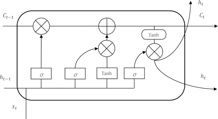
Figure 1. Fundamental structure of the LSTM network. Please click here to view a larger version of this figure.

where the forgetting gate acted as “f_t”, the input sequences as “x_t”, and “h_t-1” is the information hidden before the unit’s output. The forget gate was responsible for determining which information should be discarded or retained, the input gate could update the state of the memory unit, and the output gate could determine the value of the subsequent hidden state. These three gates are denoted as f_t, i_t, and o_t.

   (2)

  (3)

  (4)

  (5)

  (6)

Equation (3) defines the candidate cell state C'_t created by the tanh function, which proposes new values to be added to the cell state. Specifically, the model's input was formulated by integrating the outputs of two sigmoid functions with that of the initial tanh function, as depicted in Equation (5).

Equation (4) characterizes the right sigmoid function serving as the initial output value of the model, which was subsequently mapped to the interval [−1, 1] via the hyperbolic tangent function (tanh). Following this, both the resultant value from the tanh function and the output of the sigmoid function are converted to their respective actual output values, as exemplified in Equation (6).

In LSTM, the sigmoid function regulated the current information, whereas the hyperbolic tangent (tanh) function could be responsible for processing historical information. The integration of these two functions donates LSTMs with their predictive prowess. When compared to conventional RNNs, the advantage of LSTMs resides in their sophisticated architecture, which is capable of capturing the entirety of input data memory up to time step t+1. The integrity of this memory is preserved through the gating mechanism facilitated by the sigmoid function, thereby ensuring that critical information is retained over extended periods.

HP Filter
The Hodrick-Prescott filter (HP filter), proposed by Hodrick and Prescott in 1980, has been widely used in economic analysis and Time series related analysis. The HP filter assumes that the dataset to be analyzed was a combination of long-term changes and short-term fluctuations, decomposing the time series Y={y1, y2, ⋯, yT} into two subseries: the long-term trend series G={g1, g2, ⋯, gT} and the short-term fluctuation series S={s1, s2, ⋯, sT}. The long-term trend series gT, where t=1,2,⋯,T, is derived by minimizing the following expression:

 (7)

Where T represents the number of samples in the time series yt, and λ is greater than 0, known as the smoothing parameter, indicating the weights of terms  and . When λ=0, the long-term trend series G that satisfies the minimization problem is equal to the original series Y. As the value of λ increases, the total number of changes in the long-term trend series decreases relative to those in the original series, meaning that a larger λ results in a smoother long-term trend series. When λ approaches infinity, the long-term trend series will resemble a linear function. The short-term fluctuation series can be obtained by subtracting the long-term trend series from the original time series, i.e., S=Y-G.

Before applying the HP filter, it was imperative to select an appropriate smoothing parameter λ, as different smoothing parameters dictate distinct long-term trends and short-term fluctuations. In accordance with previous related research, the value of λ is set to 100 in this study.

Participant Preparation and Ethical Approval
Ethical approval had been obtained from the Inner Mongolia Medical University Ethic Review Committee (No. YKD202001041) prior to any data collection. A full-time researcher from the College of Mongolian Medicine at Inner Mongolia Medical University, skilled in the Chinese Traditional Mongolian Osteopathy (CTMO) rolling method, was recruited. Written informed consent was obtained from the participant. All procedures adhered to the principles of the Declaration of Helsinki.

Equipment Setup and Calibration
A multi-channel hand grip strength test system equipped with 24 mechanical sensors was used to collect mechanical parameters of the CTMO rolling method (refer to Figure 2 and Figure 3 for system layout and sensor positioning). All 24 force sensors were calibrated according to the manufacturer's instructions. The data acquisition software was configured to record data at a sampling frequency of 100 Hz and to display real-time force readings in Newtons (N). The recording duration was set to 60 s per trial.

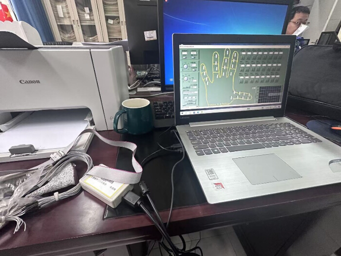
Figure 2. Multi-channel hand grip strength test system. Please click here to view a larger version of this figure.

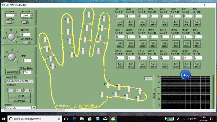
Figure 3. Massage manipulation acquisition interface based on the multi-channel grip strength test system. Please click here to view a larger version of this figure.

Data acquisition
The participant was instructed to don the instrumented glove and assume the standard starting posture. The artificial human forearm model was placed on a stable, horizontal surface in front of the participant. Upon initiation of the data recording software, the participant performed the CTMO rolling manipulation continuously on the designated area of the forearm model for 1 min. The raw data file was saved in a structured format (e.g., .csv or .txt) containing timestamps and force readings from all 24 sensors. This procedure was repeated until a total of 150 independent trials were completed. The participant rested for at least 30 s between trials to minimize fatigue-induced variability. R (version 4.2) was subsequently used to calculate movement rules and joint range-of-motion angles, and to summarize the operational characteristics of the technique.

Sensor Selection via Feature Visualization
The raw force data from all 24 sensors across all trials were loaded into R. The mean force magnitude and variance for each sensor were calculated across the entire dataset. A bubble filling diagram was constructed using the ggplot2 package in R to display the relative contribution of each finger phalanx/metacarpal to the total force exertion. Based on this diagram (Figure 4), Sensors 8 (little finger proximal phalanx), 13 (middle finger distal phalanx), and 2 (distal phalanx of index finger) exhibited the highest force magnitudes and variability and were therefore selected as the primary input features for subsequent modeling.

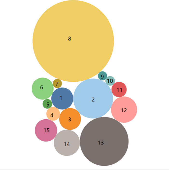
Figure 4. Bubble filling diagram of the knuckles in the rolling method. (1) proximal phalanx of index finger; (2) distal phalanx of index finger; (3) metacarpal of index finger; (4) middle phalanx of index finger; (5) ring finger proximal phalanx; (6) distal phalanx of ring finger; (7) ring finger metacarpal phalanx; (8) little finger proximal phalanx; (9) distal phalanx of little finger; (10) metacarpal of little finger; (11) middle phalanx of little finger; (12) middle finger proximal phalanx; (13) middle finger distal phalanx; (14) metacarpal of middle finger; (15) middle phalanx of middle finger. Please click here to view a larger version of this figure.

Data preprocessing for time-series modeling
The time-series force data F₈(t), F₁₃(t), and F₂(t) for the selected sensors were extracted from the raw dataset. A normalized time variable T was created by scaling the recording timestamps to the interval [0'1]. The following formula was used:

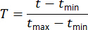
Where t was the original timestamp in seconds. For each trial, the force data and normalized time were concatenated into a multivariate time-series dataset of dimensions N × 4, where N was the number of time steps (6,000 steps for a 60 s trial at 100 Hz) and the columns corresponded to [T'F₈'F₁₃'F₂].

Hodrick–Prescott (HP) filtering
The Hodrick–Prescott filter was applied to each of the three force signals F₈, F₁₃, and F₂ independently. The smoothing parameter was set to λ = 100. This value had been chosen based on the approximate annual/cyclical nature of the long-term force trend observed in the initial 2,000 data points (as demonstrated in Figure 5) and was considered suitable for preserving biomechanical force characteristics.

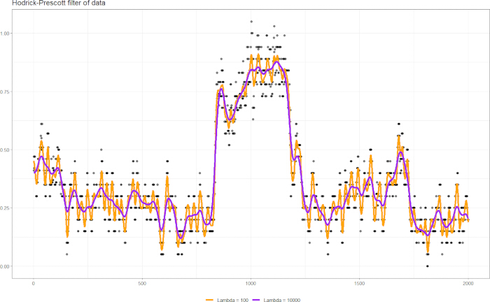
Figure 5. Comparison of HP filter effects with λ = 100 and λ = 10,000 on the first 2,000 data points from Sensor 8. Please click here to view a larger version of this figure.

Implementation note: The hpfilter function from the mFilter package in R was used with the argument freq = 100.

Two components were obtained for each sensor signal: the trend component G(t) and the cyclical component C(t), where . The final input feature matrix was constructed by concatenating the normalized time  with the HP-filtered trend and cyclical components of the three selected sensors. This resulted in a dataset of N × 7 dimensions: . The dataset was split chronologically into training (70%), validation (15%), and test (15%) subsets. Critical: Random shuffling of the time series was avoided to prevent temporal leakage. The test set contained the final 15% of the recorded time sequence.

Construction of the two-layer LSTM model with HP filtering
The computational environment was set up using TensorFlow (version 2.10) with the Keras API in R. The neural network architecture was defined as follows:
Input Layer: Shape = (sequence length'7), where sequence_length was the number of time steps per input sample (100 steps were used).
First LSTM Layer: Units = 50, return_sequences = TRUE. The tanh activation function was used for the recurrent step, and sigmoid was used for the gate activations.
Second LSTM Layer: Units = 50, return_sequences = FALSE.
Fully Connected (Dense) Layer: Units = 1 (for univariate force prediction). The complete workflow of the double-layer LSTM model with HP filtering, from data preprocessing to final prediction, is illustrated in Figure 6. The output target was the force value at Sensor 8 at the next time step (one-step-ahead prediction).

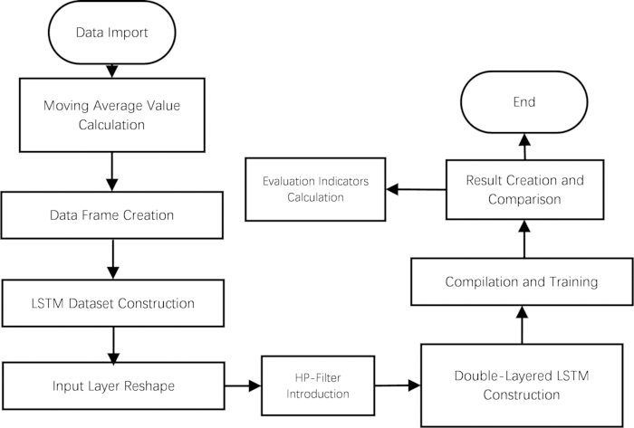
Figure 6. Double-layer LSTM application workflow chart. Please click here to view a larger version of this figure.

The model was compiled using the Adam optimization algorithm with the following hyperparameters: Learning rate: 0.001; Decay rate: 0.001; Loss function: Mean Squared Error (MSE). The model was trained for 20 epochs with a batch size of 32. Early Stopping was implemented with a patience of 5 epochs monitoring the validation loss to prevent overfitting. A Dropout rate of 0.2 was applied between the LSTM layers for regularization. The training data were shuffled only at the batch level within each epoch—not the sequential order—to maintain temporal coherence while introducing stochasticity for gradient descent.

Test dataset configuration
To evaluate the predictive performance of the proposed models, the preprocessed dataset was partitioned chronologically into three subsets: training (70%) , validation (15%) , and test (15%) . The chronological split ensured that no future information leaked into the training process. The test set comprised the final 2,000 time steps × 3 sensors = 6,000 data points of the recorded sequence, corresponding to approximately 20 s of continuous force exertion data at the original sampling rate of 100 Hz. For the evaluation of longer-duration prediction capabilities, an extended test sequence of 1,200 s (120,000 time steps) was constructed by chronologically concatenating 20 consecutive 60-s trials while preserving temporal order. Force continuity between concatenated trials was verified to ensure no abrupt transitions.

Performance metrics
Three standard regression metrics were computed to quantify prediction accuracy:

Coefficient of Determination (R²): Defined as 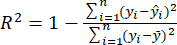, where y_i and  denote the actual and predicted force values, respectively, and  is the mean of the actual values. R² measures the proportion of variance in the force data explained by the model.

Mean Absolute Error (MAE): Defined as . MAE provides the average magnitude of prediction errors in units of Newtons (N).

Root Mean Square Error (RMSE): Defined as . RMSE is sensitive to large error deviations and is expressed in Newtons (N).

All metrics were calculated on the unseen test set after reversing any normalization or scaling transformations applied during preprocessing.

Comparative baseline models
To benchmark the proposed two-layer LSTM with Hodrick–Prescott (HP) filtering, the following alternative models were implemented and evaluated under identical training, validation, and test splits. Hyperparameters for all neural network models were tuned using the validation set to ensure a fair comparison.

Single-layer LSTM without HP filtering
Architecture: A single LSTM layer with 50 hidden units, followed by a fully connected dense layer with a single output neuron.
Input features: Raw force data from Sensors 8, 13, and 2, plus normalized time  (4-dimensional input).
Training: Adam optimizer with learning rate = 0.001, decay = 0.001, batch size = 32, trained for 20 epochs with early stopping (patience = 5) monitoring validation loss.

Double-layer LSTM without HP filtering
Architecture: Two stacked LSTM layers, each with 50 hidden units. The first LSTM layer returned full sequences, and the second LSTM layer returned only the final hidden state. A dense output layer with one neuron followed.
Input features: Same as above (4-dimensional raw force inputs).
Training parameters: Identical to the single-layer LSTM configuration.

Single-layer LSTM with HP filtering
Architecture: A single LSTM layer with 50 hidden units followed by a dense output layer.
Input features: HP-decomposed trend and cyclical components for Sensors 8, 13, and 2, plus normalized time T (7-dimensional input, as described in the Protocol).
Training parameters: Same as above.

PCA-LSTM
Dimensionality reduction: Principal Component Analysis (PCA) was applied to the 7-dimensional HP-filtered feature matrix to extract three principal components, which collectively explained >95% of the variance in the feature set.
Architecture: A single LSTM layer with 50 hidden units, taking the three principal component time series as input.
Training parameters: Same as above.

Backpropagation (BP) neural network
Architecture: A feedforward neural network with one hidden layer containing 64 neurons and ReLU activation. The output layer contained a single linear neuron.
Input representation: The time-series data were flattened into feature vectors of fixed length (100 time steps × 7 features = 700 input dimensions).
Training: Adam optimizer with learning rate = 0.001, mean squared error loss, trained for 100 epochs with a batch size of 64. Early stopping with patience = 10 was applied.

Random Forest regressor
Algorithm: Ensemble of 100 decision trees with a maximum depth of 10 and minimum samples per split set to 5.
Input representation: Same flattened feature vectors as used for the BP neural network (700-dimensional input).
Implementation: The RandomForestRegressor from the scikit-learn library (version 1.2) was employed with default hyperparameters except where specified above.

Statistical considerations
To assess the robustness of the predictive performance, each model configuration was trained and evaluated five times with different random initializations (where applicable). The reported metrics represent the mean values across the five runs, accompanied by the standard deviation to quantify variability. No cross-validation was applied to the time series to preserve temporal ordering; instead, the fixed chronological validation set was used for hyperparameter tuning.

Results

The primary model's performance was assessed using the test-set metrics. A high R² value (0.897) and low MAE/RMSE indicated that the two-layer LSTM with HP filtering successfully captured the force dynamics of the CTMO rolling method. Comparison with the baseline models showed that the HP-filtered models outperformed the non-filtered models, supporting the benefit of separating trend and cyclical components for LSTM learning. The model's performance metrics also improved as more sequential data (e.g., 1,200 s ...

Discussion

The results demonstrate that integrating a two-layer Long Short-Term Memory architecture with Hodrick–Prescott filtering substantially improves the prediction of force application in the Chinese Traditional Mongolian Osteopathy Rolling Method. Compared with single-layer and unfiltered LSTM models, the proposed combined model more effectively captured both long-term temporal dependencies and underlying trend components in force signals, leading to lower prediction errors and stronger generalization performance

Materials

List of materials used in this article

Name	Company	Catalog Number	Comments
Artificial human forearm model	Not specified	Not available	Standard training model used as the recipient surface for rolling manipulation
Keras (R package)	RStudio/Posit	CRAN: keras	Deep learning API used for LSTM model construction; version 2.10
mFilter (R package)	RStudio/Posit	CRAN: mFilter	Used for Hodrick-Prescott filtering; function hpfilter with freq = 100
Multi-channel hand grip strength test system	Zhejiang Changxian Co. Ltd.	Tekscan	24-sensor glove system for mechanical force data acquisition at 100 Hz sampling rate
neuralnet (R package)	RStudio/Posit	CRAN: neuralnet	Used for training the Backpropagation (BP) neural network baseline model
NVIDIA GeForce RTX 3060 GPU	NVIDIA Corporation	RTX 3060 (12 GB VRAM)	GPU for accelerated neural network training
Personal computer (Intel Core i7-12700, 32 GB RAM)	Intel Corporation	i7-12700	Workstation running Windows 11 for all computational experiments
Python (scikit-learn)	Python Software Foundation	scikit-learn 1.2	RandomForestRegressor implementation for the random forest baseline model
R statistical software	R Core Team	Version 4.2	Primary statistical computing environment for data preprocessing, modeling, and visualization
randomForest (R package)	RStudio/Posit	CRAN: randomForest	Alternative random forest implementation in R
TensorFlow	Google LLC	Version 2.10	Backend deep learning framework for LSTM network training