Design of DC-DC Converter for a Bifacial PV-Powered Stand-Alone Electric Vehicle Charging Station Using Secretary Bird Optimization Algorithm

Summary

This study develops a battery-storage-supported ANN-based MPPT system for a standalone electric vehicle charging station powered by a bifacial photovoltaic system. Additionally, the Secretary Bird Optimization Algorithm (SBOA) optimizes DC–DC converter, filter, and PI controller parameters to minimize total harmonic distortion (THD) and DC-bus voltage deviation.

Abstract

In response to the growing emphasis on sustainable mobility, this study presents a renewable-energy-based electric vehicle (EV) charging system incorporating a station battery energy storage (BES). The system employs a bifacial photovoltaic (PV) array with an artificial neural network (ANN)-assisted maximum power point tracking (MPPT) scheme. Additionally, the Secretary Bird Optimization Algorithm (SBOA) is used to optimize the DC–DC converter, filter, and PI controller parameters to minimize THD while maintaining a stable DC-bus voltage. Five EV models were evaluated, including one lead-acid battery-based model (BMW i3) and four lithium-ion battery-based models (Fiat 500e, Mercedes EQA 250, Volkswagen e-Golf, and Hyundai Kona Electric). The proposed MPPT configuration extracts maximum energy from the bifacial PV system while maintaining a stable DC-bus voltage under variable environmental and loading conditions. Validation through MATLAB/Simulink simulations under three operating scenarios (irradiance = 800–1000 W/m²; temperature = 20–25 °C) demonstrates high conversion efficiency, THDs of 2.85%, 2.26%, and 2.23%, and robust power management suitable for off-grid EV charging stations.

Introduction

Nowadays, integrating renewable sources, primarily solar, and EV charging stations into the distribution system is key. However, this integration leads to PQ issues and a need for advanced MPPT to extract power from renewable sources. However, due to the rapid growth in EV adoption, it became essential to have a fast, reliable charging infrastructure. The use of traditional grid-connected charging stations results in carbon emissions, stress, and power quality (PQ) issues. Additionally, integrating renewable energy sources, such as solar, with EVs can help reduce carbon emissions. However, battery storage is considered alongside solar energy, as solar energy is inherently inconsistent. AI-based MPPT techniques yield higher solar output than conventional perturb-and-observe (P & O).

A new damped fifth-order generalized integrator control algorithm for grid-integrated PV systems was proposed to accurately transfer solar power to the grid at unity PF using Human Psychology optimization¹. Besides, a learning-based hill-climbing optimal control strategy, augmented by an adaptive optimal-M Kalman filter, was employed to enhance power extraction from the PV system². On the other hand, a predictive algorithm was employed to efficiently manage and regulate power for the microgrid-integrated PV system. The system is configured with a double-stage 3φ setup³.

Meanwhile, a new voltage sensor with a lower-power-consumption approach was developed to extract the maximum output power from a solar PV system connected to an EV charging station, with a focus on efficiency and speed ⁴. However, a novel command authentication approach was devised to identify fraudulent data injection attacks that specifically target the system's centralized economic dispatch control signals⁵. Additionally, an advanced approach was introduced to derive saliency maps from interconnected solar panel arrangements and to assess the surroundings for the presence of shading⁶. A control strategy was presented to successfully manage PQ issues in the UPQC with a superconducting magnetic energy storage system, specifically with respect to load from EV charging stations⁷.

Furthermore, the bifacial PV module poses a significant challenge to the financial viability of PV. While forecasting methods for monofacial PV performance are well established, adapting these models to bifacial systems is still in progress^8,9. Moreover, multiple studies have shown that bifacial PV energy production is influenced by geometric factors. It is important to consider these elements when assessing the operation of bifacial technologies^{10,11,12,13,14,15}. On the other hand, P & O and AI-based MPPT were developed for PV power extraction in addition to the design of controllers with optimization methods^16,17,18. Modeling and simulation of bifacial PV with monofacial PV is discussed in detail¹⁹. Meanwhile, P & O and ANN-based MPPT for PV systems were suggested for EV charging station design^20,21. The PV power EV charging station was designed to support various models with the P & O MPPT²². Next, the behavior of the secretary bird for its survival, such as searching and hunting prey, is mathematically modeled for SBOA²³. A new fuzzy-logic-regulated DC-DC converter was presented for constant charging of a solar-supported house²⁴. The direct flow and torque control diagram introduced fuzzy logic to cover the vehicle's torque demand and optimized training performance²⁵.

Besides, a comprehensive review of emerging trends, including vehicle-to-grid (V2G) technology and AI-controlled energy management systems, as well as the role of renewable sources in grid-responsive EV operations, was conducted²⁶. Furthermore, a new method was developed to address uncertainties in renewable power generation, EV charging behavior, and market pricing²⁷. However, the key differences between EVs and SAEVs in V2G technology, with SAEVs' novel method with distinct features, were discussed, which enhanced their role in V2G integration²⁸.

Several studies have been conducted on monofacial PV-powered grid-connected EV charging stations using conventional MPPT methods, such as P & O (listed in Table 1), I & C, Fuzzy, and metaheuristic optimization methods. They focused either on the PV power extraction system or on controller parameter selection. However, only a few monofacial PV systems with AI-based MPPT and optimal parameter selection for DC-DC converters, filters, and PI control gains, all within a single framework, are available to maintain DC bus voltage stability and reduce THD. Therefore, this research gap motivates the development of an ANN-based MPPT for Bifacial PV and optimized controllers for converters and filters to enhance PQ in a standalone EV charging station operating under dynamic conditions. This study presents a stand-alone bifacial PV charging architecture integrated with an artificial neural network-driven MPPT controller, designed for highway-based EV stations. The system is configured to charge five EV battery types²², including four lithium-ion models: Hyundai Kona Electric, Volkswagen e-Golf, Fiat 500e, Mercedes EQA 250, and BMW i3, and one lead-acid configuration, supported by an auxiliary battery-storage module that ensures stable operation under fluctuating solar conditions.

The major contributions of the proposed work can be mentioned as follows: (1) Development of a BES-supported bifacial PV arrangement operating in isolated mode to deliver energy to multiple EVs and to a station-level AC demand through coordinated DC/AC interfaces. Bifacial PV harvests more energy from both the front and rear surfaces than monofacial PV. (2) Implementation of an ANN-based MPPT algorithm that adaptively regulates the boost-converter duty ratio to extract maximum available solar power. (3) Optimization of DC-DC converter parameters, R L values of filter, and PI-controller gains via the Secretary Bird Optimization Algorithm (SBOA), targeting low THD and steady DC-bus voltage during irradiance and temperature variations.(4) Validation through three operating scenarios involving variable environmental and load conditions to evaluate controller robustness and system efficiency.

Protocol

In this research, a stand-alone bifacial PV- and battery energy storage system (BESS)-fed EV charging system is developed, as shown in Figure 1, using an ANN-controlled MPPT method. A single-diode equivalent circuit is used to model the bifacial PV array, accounting for temperature, series resistance, shunt resistance, solar irradiance, and rear-side irradiance. The PV output is supplied to the EV charging station through a DC–DC boost converter, while the BESS supports DC-bus voltage regulation. The Secretary Bird Optimization Algorithm (SBOA) is used to optimize the PI controller gains and filter parameters. The modeling of the system components and the proposed methodology are described in the following subsections.

Modeling of Components

1. Bifacial PV system

The PV modules help to achieve the required current and voltage output. In the present study, two monofacial PV modules were used to emulate the energy generation characteristics of bifacial arrays under different surface-albedo conditions⁹. The bifacial gain of irradiance BG_g is determined by Equation (1)

   (1)

Here, front irradiation is G_f, and rear irradiance is G_r. Maximum bifacial PV current is I_mp, and voltage is V_mp. Finally, the output produced by the bifacial system with the chosen number of series N_s and parallel N_p modules are given by Equation (2). The control of PV is given in Figure 2

   (2)

2. Battery storage system (BSS)

Batteries are a crucial means of storing electrical energy¹⁸ . This work uses Li-ion batteries as the energy storage system. Among the available rechargeable battery options, this work focuses on Li-ion batteries, which are considered optimal for EVs due to their efficiency and power density. Equations (3) and (4) describe the Li-ion battery with constraints.

  (3)

The specifications of the PV, storage battery, and converter are summarized in Table 2, while Table 3 presents the power-flow allocation among the PV array, energy-storage unit, and connected loads.

   (4)

3. DC –AC converter

The Neutral-Point-Clamped (NPC) inverter is widely adopted in modern power conversion systems for renewable energy. Compared with the conventional two-level structure, the NPC configuration offers reduced total harmonic distortion (THD), lower electromagnetic interference, and lower voltage stress on semiconductor devices. The DC link of this topology is divided into three potential levels +Vdc/2, 0, and -Vdc/2, by means of paired capacitors and clamping diodes forming the neutral junction. By appropriately controlling the switching, the inverter generates three discrete voltage states at the output terminals, thereby improving waveform quality and power conversion efficiency. The neutral point of the DC bus in an NPC inverter plays a key role in balancing capacitor voltages and ensuring proper inverter operation. The inverter's control scheme is shown in Figure 3.

4. DC-DC Boost Converter

DC-DC converters step up the input DC voltage to a higher output voltage by controlling the duty cycle of a high-frequency switching device while maintaining efficiency. It has two operating modes. During the ON state, the diode is reverse-biased, and the input source supplies energy to the inductor, which stores it as a magnetic field, while the output capacitor supplies energy to the load. During the OFF state, the diode becomes forward-biased. Here, energy stored in the inductor is released through the diode to the capacitor connected at the output and load, combining with the input source to produce an output greater than the input voltage. By varying the PWM duty cycle, the converter's output voltage varies according to the relation , where D is the duty cycle. It is used in solar, fuel cell, EV, and storage systems.

ANN control scheme for MPPT

In this work, an ANN-based MPPT is selected to collect the maximum power generated from the solar system¹⁷. Irradiation and temperature datasets used for ANN training were generated in MATLAB/Simulink under varying environmental operating conditions, corresponding to solar irradiance levels of 800–1000 W/m² and temperature ranges of 20–25 °C, with a duty cycle (D). The ANN is trained to minimize the MSE between the obtained and required outputs (O_p, ) to extract maximum power from the bifacial PV system. Here, the solar irradiation and temperature are used as inputs to the ANN, and the duty cycle is the output to control the boost converter. The structure of the developed ANN model for MPPT, as given in Figure 4, is considered in the work. Supplementary Table 1 presents the advantages and disadvantages of the proposed method compared with other standard methods.

An ANN consists of three main layers: an output layer (OPL), an input layer (IPL), and a hidden layer (HIL). This helps to transfer the data between the IPL and HIL. Subsequently, it is produced by the weights in the links connecting the IPL and HIL. In this context, computations are executed with a certain bias applied to the HL variable, and the resulting outcomes are accumulated in the OPL variable. Here, the LMBP-type ANN [17] is selected. The connection weights are tuned throughout training by measuring the error to achieve the target output. Here, LMBP is used to train ANNs with the MSE as the performance function. The LMBP algorithm utilizes the derived derivatives to update the weights, which exhibit the properties of effective learning and accelerated convergence

Every neuron in a multilayer perceptron network has a summation and an activation function. Nevertheless, there are certain numerical weights (w_pk) that connect these neurons across the levels. When inputs are multiplied by weights as specified in Equation (5). The nonlinear sigmoid function is considered with MSE minimization given in Equation (6).

   (5)

    (6)

SBOA optimized the filter and control parameters of the proposed system

These days, metaheuristic algorithms play a key role in solving engineering problems. Figure 5 gives a classification of algorithms. SBOA algorithm²³ mimics the behavior of the SB to survive in its natural habitat. The exploration and exploitation stages of the Secretary Bird's hunting behavior are modeled in SBOA. The algorithm's exploration phase mimics the SB behavior of catching snakes, while its exploitation phase mimics their behavior of dodging predators like eagles. The solution process begins by generating random values within their respective limits for each SB in the population, and by calculating the objective function value by running the Simulink model, treating each SB's value as a design parameter. Based on the objective value, each SB changes its position to represent a better solution. The SBOA mathematical modeling is discussed below:

Initial preparation phase

First, it is necessary to identify the initial solutions that were utilized to begin the search for a typical minimization of the objective function F(Y). In this case, the initial random population Y = [Y₁, Y₂, ......Y_N] of SB‘s is formed via N initial solutions. Equation (7) initializes the population and Y_i in the represents a solution.

   (7)

Where the choice variables' lower and upper bounds are denoted by lb and ub. In [0, 1], r is a random number. N Is the problem's dimension. Furthermore, the solution's fitness value F_i = F(Y_i) is used to quantify the quality of Y_i.

Hunting strategy of SB’s

Finding, eating, and assaulting the prey are the three main phases of SB hunting. The entire hunting process has been divided into three equal time intervals, t < 1/3T, 1/3T < t < 2/3T, and 2/3T < t < T. Here, t is the current iteration, and T is the maximum number of iterations. These intervals correspond to the three phases of the SB's predation: searching, consuming, and attacking prey. These divisions are based on the biological statistics of the bird's hunting phases and the time durations of each phase. Consequently, the following is how each SBOA phase is modeled:

Searching for prey

The SB must hunt prey from a safe distance during this phase. To gather sufficient data across the entire search region, the first step in optimization algorithms requires stronger exploration. By using the locations of the other two SB’s as a guide, the SB can investigate additional possible regions. To further increase algorithm diversity, differential mutation processes are thus introduced. When t is less than 1/3rd of T, Equation (8) is used to update the position of each individual. It will search for, consume, and assault prey. Consequently, the following is how each SBOA phase is modeled:

 (8)

Where, Y_i(t) is the current position of the i^th SB, Y^new_i(t) gives the updated solution, two individuals Y_i(t), Y_r2(t) were randomly chosen from the existing population. A random vector, for the parameter-selection strategy, R₁ has 1 × N randomly chosen from [0, 1] for effective balance among exploitation and exploration phases. The updated solution is considered only if it results in an improved objective value compared to the previously obtained solution.

Consuming prey

SB uses nimble agility and moves to hover around the snake after spotting possible prey. The prey's patience will be used to lower its defenses by observing and enticing opponents as they circle. Other SB’s adjust their posture near the prey. Hunting success will be significantly increased with this approach. Equation (9) illustrates how the Brownian motion (B) is used to simulate the SB’s random movement when 1/3 T < t < 2/3 T.

 (9)

Where the B is implemented in MATLAB using the standard normal distribution by the randomly generated vector r(1,M). SB’s then use Equation (10) to update their positions.

 (10)

Where, Y_best(t) is the best solution and the exponential scaling factor exp((t/T)⁴) is chosen to increase the exploitation capacity for every iteration.

Attacking prey

After consuming continuously, the victim will run out of energy. The secretary birds should launch the assault now. Here, different attack methods, such as incessant steps /sporadic long jumps over a short time period, are simulated using the Lévy flight technique. The characteristics are described by Equations (11) and (12). Candidate options are near the optimal answer at the moment because SB’s swiftly approach the prey. This plan will be implemented when t > 2/3T.

 (11)

 (12)

Where, LF represents the Levy flight strategy and , s= 0.01, and φ = 1.5 fixed values. μ and υ are arbitrary values that lie in [0, 1]. Where, τ denotes gamma and η = 0.5, the weighting factor 0.5 was adopted, as proposed in the original SBOA formulation, to regulate the step size and maintain a balance between large exploratory jumps and local refinement. Table 4 presents the values used for the ANN and the SB algorithm in the developed system.

Escape strategy for SB

When hunting other prey in the wild, SBs risk being hunted. Eagles, hawks, foxes, and jackals are the primary adversaries they must contend with. They must use a variety of evasion techniques to safeguard themselves or their prey when they perceive danger. This algorithm simulates the escape methods by modeling running modes (D₂) and camouflage (D₁). When facing adversaries, secretary birds initially blend into their surroundings to stay safe. Here, secretary birds strive to avoid local optima in the algorithms by updating their positions around the prey (the best individual). They will use flight or rapid-running tactics to stay safe if they are unable to evade the enemy. For reference, a random individual Y_rand is chosen as the leader to avoid being restricted to a local optimum. Equations (13) and (14) are used by secretary birds to update their positions. The SBOA flowchart is shown in Figure 6.

    (13)

   (14)

Representation of design variables

The problem variables in this study include the design parameters, such as the PI controller gains of DC-DC converters, as well as the resistances and inductances of filters and converters. Equation (15) gives the representation of control variables. The control parameter bonds are listed in Supplementary Table 2.

    (15)

Fitness function (FF)

The minimization of THD is selected as the objective function (Obj) in this study. The maximum value of FF is the minimum value of Obj, given in Equation (16) and (17).

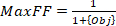    (16)

     (17)

Results

The proposed stand-alone Bifacial PV system with ANNC-based MPPT for an EV charging station was constructed in Simulink/Matlab 2022b and executed on an Intel Core i7 with 16GB RAMS. The selected system and EV load ratings are displayed in Table 2 and Supplementary Table 3. In this work, three cases listed in Table 5 with various permutations of solar irradiation (G), temperature (T), AC loads, and five EV cars from different models and ratings are used to demonstrate the system's perform...

Discussion

Overall, the outcomes indicate that this research work contributes to the scientific field by introducing a novel, optimized control strategy that enhances solar output, improves PQ, and supports a sustainable EV charging infrastructure appropriate for highways. The developed ANN-based MPPT with SBOA-optimized filter, converters, and controller achieves lower THD while maintaining a stable DC bus voltage for PV- and BES-supported standalone EV charging station¹⁷.

Litera...

Materials

List of materials used in this article

Name	Company	Catalog Number	Comments
DC–AC converter	MathWorks	Simscape Electrical Three-Level Converter documentation: https://www.mathworks.com/help/sps/ref/threelevelconverterthreephase.html	Three-phase, three-level neutral-point-clamped DC–AC converter model.
DC–DC converter	MathWorks	Simscape Electrical Boost Converter documentation: https://www.mathworks.com/help/sps/ref/boostconverter.html	Boost DC–DC converter model used to regulate the PV output voltage.
EV1 battery	MathWorks	Battery model documentation: https://www.mathworks.com/help/autoblks/ref/datasheetbattery.html	Simulated lead-acid battery representing EV1.
EV2–EV5 batteries	MathWorks	Battery model documentation: https://www.mathworks.com/help/autoblks/ref/datasheetbattery.html	Simulated lithium-ion battery models representing EV2, EV3, EV4, and EV5.
MATLAB/Simulink	MathWorks	Software; https://www.mathworks.com/products/simulink.html	Software environment used to model and simulate the PV-powered electric-vehicle charging station.
Simscape Electrical	MathWorks	Software; https://www.mathworks.com/products/simscape-electrical.html	Component library used to model the power converters, electrical network, and associated control system.
Solar panel	Waaree Energies Ltd.; modeled in MATLAB/Simulink	Model WSM-315. Waaree product information: https://www.waaree.com/solar-pv-modules/; System Advisor Model: https://sam.nrel.gov/	WSM-315 solar panel parameters were entered as a user-defined PV module using data from the Waaree datasheet and the NREL System Advisor Model.
Storage battery	MathWorks	Lead-acid battery model documentation: https://www.mathworks.com/help/simscape/ug/lead-acid-battery.html	Simulated lead-acid battery used as the stationary energy-storage system.

References

- Kumar N, Singh B, Panigrahi BK. Grid synchronization framework for partially shaded solar PV-based microgrid using intelligent control strategy. IET Gener Transm Distrib. 2019;13(6):829-837.
- Kumar N, Singh B, Wang J, Panigrahi BK. A framework of L-HC and AM-MKF for accurate harmonic supportive control schemes. IEEE Trans Circuits Syst I Regul Pap. 2020;67(12):5246-5256.
- Saxena V, Kumar N, Singh B, Panigrahi BK. An MPC-based algorithm for a multipurpose grid integrated solar PV system with enhanced power quality and PCC voltage assist. IEEE Trans Energy Convers. 2021;36(2):1469-1478.
- Kumar N, Singh B, Panigrahi BK. Voltage sensorless model predictive control with battery management system for solar PV-powered onboard EV charging. IEEE Trans Transp Electrif. 2023;9(2):2583-2592.
- Siu JY, Kumar N, Panda SK. Command authentication using multiagent system for attacks on the economic dispatch problem. IEEE Trans Ind Appl. 2022;58(4):4381-4393.
- Hole SR, Goswami AD. Design of an efficient MPPT optimization model via accurate shadow detection for solar photovoltaic. Energy Harvest Syst. 2023;10(2):377-383.
- Çelik D, Ahmed H. Enhanced control of superconducting magnetic energy storage integrated UPQC for power quality improvement in EV charging station. J Energy Storage. 2023;62:106843.
- Bouchakour S, Caballero DV, Luna A, Medina ER, El Amin KB, Cortes PR. Monitoring, modelling and simulation of bifacial PV modules over normal and high albedos. In: Proc 9th Int Conf Renew Energy Res Appl (ICRERA); 2020 Sep 27-30; Glasgow, UK. p. 252-256.
- Shoukry I, Libal J, Kopecek R, Wefringhaus E, Werner J. Modelling of bifacial gain for stand-alone and in-field installed bifacial PV modules. Energy Procedia. 2016;92:600-608.
- Yusufoglu UA, Pletzer TM, Koduvelikulathu LJ, Comparotto C, Kopecek R, Kurz H. Analysis of the annual performance of bifacial modules and optimization methods. IEEE J Photovolt. 2015;5(1):320-328.
- Luque A, Lorenzo E, Sala G, López-Romero S. Diffusing reflectors for bifacial photovoltaic panels. Sol Cells. 1985;13:277-292.
- Chieng YK, Green MA. Computer simulation of enhanced output from bifacial photovoltaic modules. Prog Photovolt Res Appl. 1993;1(4):293-299.
- Yusufoglu UA, Lee TH, Pletzer TM, Halm A, Koduvelikulathu LJ, Comparotto C, et al. Simulation of energy production by bifacial modules with revision of ground reflection. Energy Procedia. 2014;55:389-395.
- Janssen GJ, Van Aken B, Carr AJ, Mewe AA. Outdoor performance of bifacial modules by measurements and modelling. Energy Procedia. 2015;77:364-373.
- Lave L, Samuel M, Stein S, Burnham J. Performance Results for the Prism Solar Installation at the New Mexico Regional Test Center: Field Data from February 15-August 15, 2016. Albuquerque (NM): Sandia National Laboratories; 2016.
- Srilakshmi K, Jyothi KK, Kalyani G, Goud YSP. Design of UPQC with solar PV and battery storage systems for power quality improvement. Cybern Syst. 2023; 56(5):599-628
- Srilakshmi K, Sujatha CN, Balachandran PK, Mihet-Popa L, Kumar NU. Optimal design of an artificial intelligence controller for solar-battery integrated UPQC in three-phase distribution networks. Sustainability. 2022;14(21).
- Srilakshmi K, Srinivas N, Balachandran PK, Reddy JGP, Gaddameedhi S, Valluri N, et al. Design of soccer league optimization-based hybrid controller for solar-battery integrated UPQC. IEEE Access. 2022;10:107116-107136.
- Bouchakour S, Valencia-Caballero D, Luna A, Roman E, Boudjelthia EAK, Rodríguez P. Modelling and simulation of bifacial PV production using monofacial electrical models. Energies. 2021;14(14):4224. doi:10.3390/en14144224.
- Dineshraj V, Prasanna Moorthy V. ANN-based MPPT for electric vehicle charging station. Int J Adv Res Sci Commun Technol. 2022;2(1):721-728. doi:10.48175/IJARSCT-4652.
- Rashid A. A grid-integrated PV-powered EV charging station featuring artificial neural network-based MPPT and comprehensive power flow control. E3S Web Conf. 2025;650:01015. doi:10.1051/e3sconf/202565001015.
- Awad M, Ibrahim AM, Alaas ZM, El-Shahat A, Omar AI. Design and analysis of an efficient photovoltaic energy-powered electric vehicle charging station using perturb and observe MPPT algorithm. Front Energy Res. 2022;10:969482. doi:10.3389/fenrg.2022.969482.
- Fu Y, Liu D, Chen J, et al. Secretary bird optimization algorithm: A new metaheuristic for solving global optimization problems. Artif Intell Rev. 2024;57:123. doi:10.1007/s10462-024-10729-y.
- Vidia Laksmi BN. Design of automatic battery charger using forward DC-DC converter for solar home energy. Vokasi UNESA Bull Eng Technol Appl Sci. 2025;2(1):57-66.
- Araria R, Berkani A, Negadi K, Marignetti F, Boudiaf M. Performance analysis of DC-DC converter and DTC-based fuzzy logic control for power management in electric vehicle application. J Eur Syst Autom. 2020;53(1):1-9. doi:10.18280/jesa.530101.
- Satpathy PR, Ramachandaramurthy VK, Radha Krishnan TR, et al. Technological innovations and sustainable strategies for advancing electric vehicle performance and market integration. Energy Strategy Rev. 2025;60:101790. doi:10.1016/j.esr.2025.101790.
- Saheb GM, Jamiu O, Li L. A review on electric vehicle charging station operation considering market dynamics and grid interaction. Appl Energy. 2025;392:126058. doi:10.1016/j.apenergy.2025.126058.
- Radha Krishnan TR, Satpathy PR, Ramachandaramurthy VK, Dollah Z, Pulenthirarasa S, Ramasamy A. Optimizing vehicle-to-grid systems: Smart integration of shared autonomous and conventional electric vehicles. eTransportation. 2025;24:100401. doi:10.1016/j.etran.2025.100401.
Access restricted. Please log in or start a trial to view this content.