A Nonlinear Dynamic System Modeling of Stress Regulation and Emotional Behavior in Higher Education

Summary

This protocol presents a physics-inspired nonlinear state-space framework for modeling stress–emotion dynamics in higher education, enabling users to analyze burnout thresholds, oscillatory stress cycles, resilience, and adaptive regulation using differential equations, stability analysis, and stochastic simulations.

Abstract

Stress regulation and emotional behavior in higher education are commonly examined using descriptive statistical models that lack a mechanistic dynamical structure. However, academic stress exhibits nonlinear behaviors, including threshold effects, burnout, and adaptive responses, that are not adequately captured by linear models. This study adopts a nonlinear dynamical systems perspective to model stress regulation and emotional behavior in higher education. The primary aim of this study is to develop a physics-inspired nonlinear state-space framework that rigorously models stress–emotion coupling and adaptive regulation in higher education. The protocol establishes a nonlinear state-space model describing stress, emotional activation, and regulatory capacity. Users can implement the protocol to simulate system dynamics and evaluate stability under varying academic conditions. The framework incorporates nonlinear stability analyses and stochastic simulations to investigate resilience, instability, and burnout-related transitions. Simulation results demonstrate nonlinear stability, resilience effects, and regime transitions that are not captured by conventional linear models. The results indicate that stress regulation in higher education behaves as a nonlinear dynamical system. By integrating nonlinear dynamics, energy landscape modeling, and adaptive regulation theory, this work provides a unified predictive framework that explains resilience, instability, and recovery processes in academic environments. The framework provides a foundation for future studies of student wellbeing and burnout risk. The framework is relevant to researchers and practitioners interested in student well-being and stress regulation.

Introduction

Stress regulation and emotional behavior in higher education can be interpreted as a complex dynamical process that evolves over time under the combined influence of internal psychological feedback and external academic pressures¹. Coursework, examinations, institutional expectations, and social evaluation continuously perturb students' emotional states, producing fluctuations in anxiety, motivation, and engagement². These emotional responses evolve within a multidimensional phase space governed by cognitive appraisal, coping strategies, and adaptive regulation mechanisms³. Classical stress-response models in educational psychology typically assume proportional relationships between stress stimuli and emotional reactions, often relying on regression analyses or descriptive statistical indices to characterize these relationships⁴. However, empirical observations consistently demonstrate nonlinear features such as threshold effects, saturation, hysteresis, and abrupt transitions, including burnout and emotional collapse⁵. Small stressors may produce negligible emotional shifts under stable conditions; however, near critical thresholds, they can trigger disproportionate emotional responses⁶. Such behavior resembles nonlinear oscillations and bifurcation phenomena observed in physical systems maintained far from equilibrium⁷. Within this perspective, students may be conceptualized as open dissipative systems that continuously exchange stress-related "energy" with their academic environment through feedback processes governing regulation and adaptation⁸.

From an educational and psychological perspective, the concepts used in the present framework can be interpreted intuitively. Stress accumulation represents the progressive burden generated by academic demands and environmental pressures. Emotional activation reflects changes in affective states, such as anxiety, frustration, motivation, and engagement, whereas regulatory capacity corresponds to the coping and self-regulation mechanisms that help students adapt to challenges. For future empirical implementation, stress accumulation may be represented using perceived stress scales; emotional activation may be assessed using validated anxiety, mood, or emotional well-being instruments; and regulatory capacity may be estimated using resilience, coping, or self-regulation measures. These mappings provide a practical foundation for future parameter estimation and model calibration. Within this context, nonlinear concepts such as stability, resilience, and critical transitions can be understood as distinct patterns of psychological adaptation. Stable states represent balanced emotional functioning, resilience reflects the ability to recover from disturbances, and critical transitions correspond to abrupt shifts toward maladaptive outcomes, such as chronic stress or burnout. These interpretations establish a clearer conceptual bridge between educational psychology and nonlinear dynamical systems theory, thereby improving the accessibility of the proposed framework for interdisciplinary audiences.

To provide a conceptual overview of these interactions, Figure 1 illustrates the structure of dynamical stress–emotion interactions in higher education systems. The diagram presents stress inputs stemming from academic demands, emotional response variables representing the evolution of psychological state, and adaptive regulatory mechanisms that modulate the system through feedback loops. These components interact dynamically, producing trajectories within a stress–emotion phase space that may converge toward stable emotional states or diverge toward maladaptive regimes. Although this conceptual representation highlights the dynamic nature of emotional regulation, existing psychological models rarely translate these relationships into explicit mathematical structures that describe temporal evolution.

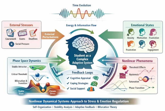
Figure 1: Conceptual diagram of dynamical stress–emotion interaction in higher education systems. This figure illustrates the conceptual structure of stress–emotion dynamics in academic environments. The diagram shows stress inputs originating from academic demands, emotional response variables representing the evolution of psychological states, and adaptive regulatory mechanisms that modulate the system through feedback loops. Please click here to view a larger version of this figure.

The limitations of current modeling approaches are further illustrated in Figure 2, which presents a conceptual framework identifying the major research gaps in the existing stress-modeling literature. At the center of the diagram lies the absence of a mechanistic dynamical framework for stress–emotion interaction. Surrounding this limitation are several interconnected gaps that characterize current research. First, many studies rely on correlation-based stress indices that lack governing equations to describe time evolution and feedback dynamics⁹. Second, burnout and emotional instability are frequently described qualitatively rather than through formal stability analysis using Jacobian matrices or eigenvalue-based criteria¹⁰. Third, existing models lack energy landscape representations capable of quantifying resilience or basin-of-attraction geometry within emotional regulation systems¹¹. Finally, stress and emotional responses are often treated as independent variables rather than as dynamically coupled state variables governed by nonlinear feedback processes¹². Together, these gaps highlight the need for a rigorous dynamical modeling framework capable of describing oscillatory behavior, multistability, and phase transitions in higher-education stress systems.

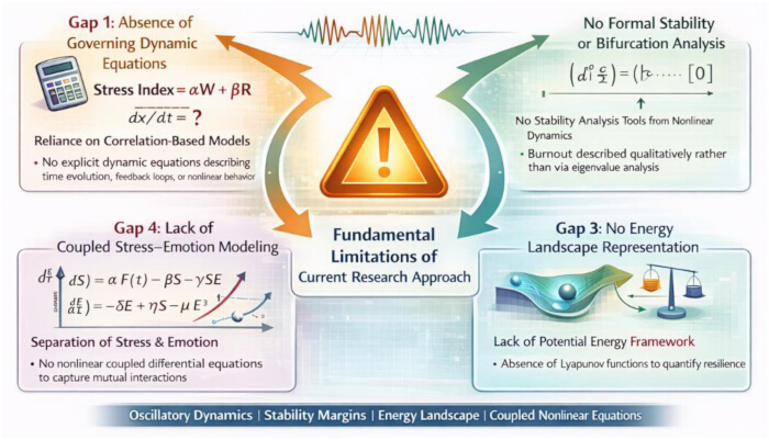
Figure 2: Conceptual framework illustrating research gaps in existing stress modeling literature. This figure presents a conceptual overview of the main limitations in current stress modeling approaches. At the center of the diagram is the absence of a mechanistic dynamical framework describing stress–emotion interaction. Please click here to view a larger version of this figure.

To address these limitations, Figure 3 presents the proposed nonlinear dynamical modeling architecture developed in this study. The framework integrates stress accumulation dynamics, emotional activation variables, and adaptive regulatory feedback mechanisms within a unified nonlinear state-space formulation. Within this framework, the evolution of the system can be described through nonlinear differential equations that capture internal regulation dynamics, external forcing effects, and stochastic perturbations arising from unexpected academic events. Such a formulation allows stress–emotion interactions to be analyzed using tools from nonlinear dynamical systems theory, including equilibrium analysis, bifurcation analysis, Lyapunov stability theory, and stochastic stability methods^13,14,15,16. By introducing explicit governing equations, the model enables rigorous analysis of how emotional states evolve over time under continuous environmental forcing and internal feedback processes.

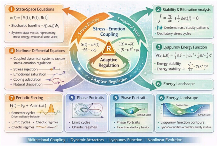
Figure 3: Proposed nonlinear dynamical modeling architecture for stress–emotion regulation. This figure illustrates the nonlinear dynamical framework developed in this study for modeling stress–emotion interactions in higher education systems. The architecture integrates stress-accumulation dynamics, emotional-activation variables, and adaptive regulatory feedback mechanisms into a unified state-space formulation. Please click here to view a larger version of this figure.

The overall goal of the method presented in this work is to establish a mechanistic nonlinear modeling framework that enables the analysis of stress regulation in higher education as a dynamical system capable of exhibiting multistability, oscillatory regimes, and critical transitions. Unlike conventional linear stress-index models, the proposed framework explicitly incorporates nonlinear feedback interactions among accumulated stress energy, emotional activation, and adaptive regulation capacity^17,18,19,20. These nonlinear interactions enable the identification of equilibrium states, the characterization of stability margins, and the detection of tipping points associated with burnout transitions. In addition, the framework introduces an energy-landscape interpretation of emotional regulation in which Lyapunov-type potential functions describe the stability structure of emotional states^21,22,23. Within this representation, resilience can be quantified by basin-of-attraction depth, whereas instability thresholds correspond to bifurcation points at which stable attractors disappear.

To enhance realism, the model incorporates periodic forcing terms representing academic semester cycles, as well as stochastic perturbations that capture unexpected academic events or environmental fluctuations^24,25,26. These extensions allow the framework to simulate realistic academic stress dynamics, including oscillatory stress cycles during examination periods and noise-driven transitions between emotional states. Such modeling capabilities provide advantages over purely statistical approaches by enabling predictive analyses of instability thresholds and resilience mechanisms.

Nonlinear dynamical approaches have previously been applied in fields such as biological regulation, neuroscience, and complex social systems, where feedback-driven processes produce emergent behaviors that cannot be explained using linear models^27,28,29. Applying similar principles of stress regulation in higher education bridges educational psychology and dynamical systems theory, enabling the analysis of emotion regulation processes within a mathematically rigorous framework. By combining nonlinear dynamical modeling, stability theory, and energy landscape analysis, the method described here provides a unified platform for investigating stress dynamics, resilience mechanisms, and emotional stability in academic environments³⁰.

Ultimately, this framework enables researchers to analyze how stress accumulates, how emotional responses evolve, and how adaptive regulatory mechanisms influence long-term system stability. The approach, therefore, offers a powerful methodological tool for studying resilience, burnout transitions, and recovery processes in higher education systems. Beyond its methodological contribution, the proposed framework is intended to serve as an interdisciplinary bridge between educational psychology and nonlinear dynamical systems science. By translating psychological processes such as stress accumulation, emotional activation, resilience, and adaptive regulation into mathematically tractable state variables, the framework provides a common analytical language for investigating complex educational phenomena with rigorous dynamical tools. This integration enhances conceptual clarity, facilitates future empirical calibration using behavioral and psychological measurements, and supports the development of predictive and explanatory models for stress regulation in academic environments³¹. In simple terms, the proposed framework examines how academic stress accumulates, how emotional responses change over time, and how coping mechanisms influence recovery and resilience. The model aims to identify conditions under which students maintain emotional stability or become vulnerable to burnout, thereby bridging psychological theory and quantitative systems analysis.

Protocol

This protocol does not involve human or animal experimentation. The study relies exclusively on mathematical modeling and computational simulation of stress–emotion dynamics in higher education systems. The computational tools, software environments, and numerical resources required to implement the nonlinear dynamical modeling framework described in the protocol are listed in the Table of Materials.

1. Model initialization and computational environment setup

1. Open the computational environment and create a new project directory for the simulation study. Complete software details are provided in Supplementary File 1.
2. Create a primary script file named StressEmotionModel.m for implementation of the nonlinear stress–emotion–regulation framework.
3. Define the three state variables representing the dynamical system.
   1. Define S(t) as accumulated academic stress. Define E(t) as emotional activation.
   2. Define R(t) as adaptive regulatory capacity.
4. Create a parameter initialization file and assign values to all baseline model parameters.
5. Define the baseline parameter set as follows.
   1. Set the external forcing parameter F to 2.0. Set the stress dissipation parameter β to 0.30.
   2. Set the stress–emotion coupling parameter γ to 0.50. Set the regulation gain parameter κ to 0.40.
   3. Set the emotional sensitivity parameter α to 0.80. Set the emotional relaxation parameter δ to 0.50.
   4. Set the nonlinear saturation parameter µ to 0.10. Set the regulation-mediated interaction parameter η to 0.20. Set the regulation decay parameter λ to 0.25.
6. Define the initial state vector.
   1. Set S(0) = 1.0.
   2. Set E(0) = 0.5.
   3. Set R(0) = 0.8.
      NOTE: Use identical parameter values across all baseline simulations unless conducting a sensitivity analysis.

2. implementation of the nonlinear dynamical model

1. Create a function file containing the coupled differential equations governing stress, emotion, and regulation dynamics. The governing equations are provided in Supplementary File 1 (Section S1.2), while the corresponding MATLAB implementation is presented in Supplementary File 1 (Section S1.8).
   NOTE: The baseline model parameters, initial conditions, numerical solver configuration, and governing nonlinear ordinary differential equations are provided in Supplementary File 1 (Sections S1.2–S1.6). These parameters are used consistently throughout all numerical simulations unless otherwise specified.
2. Implement the stress evolution equation for the accumulated stress state variable S(t) according to the governing nonlinear dynamical system described in Supplementary File 1, Section S1.2. The corresponding computational implementation of this equation is provided in Supplementary File 1, Section S1.8 (Function 1: Model Equations).
3. Implement the emotional activation equation described in Supplementary File 1, Section S1.2. The MATLAB implementation of the emotional activation equation is available in Supplementary File 1, Section S1.8 (Function 1: Model Equations).
4. Implement the adaptive regulation equation governing the regulatory capacity state variable R(t) according to the nonlinear model described in Supplementary File 1, Section S1.2. The corresponding MATLAB implementation is provided in Supplementary File 1, Section S1.8 (Function 1: Model Equations).
5. Enable optional stochastic perturbations by introducing independent Gaussian noise terms into each state variable to simulate random academic disturbances and environmental variability.
6. Perform 30 independent stochastic realizations (n = 30) using different random noise sequences while maintaining identical baseline model parameters and initial conditions.
7. Compute the mean trajectories and the corresponding variability estimates, with the error bars reported in the Results section representing the statistical variation across these independent realizations.
8. Integrate the nonlinear dynamical system using the ODE45 numerical solver with a relative tolerance of 1 × 10⁻⁶, an absolute tolerance of 1 × 10⁻⁸, an initial integration step of 0.001, and a maximum step size of 0.05 over the simulation interval 0 ≤ t ≤ 500.
9. Provide the detailed computational implementation, solver configuration, and simulation workflow in Supplementary File 1, Sections S1.6–S1.11.
10. Define the stochastic amplitudes as follows.
    1. Set σS = 0.05.
    2. Set σE = 0.05.
    3. Set σR = 0.03.
11. Constrain all state variables to remain non-negative during numerical integration.
12. Replace negative numerical values with zero during post-processing.

3. Numerical simulation

1. Configure the numerical solver.
   1. Select ODE45 for deterministic simulations.
   2. Select an equivalent stochastic integration routine when stochastic simulations are performed.
   3. Determine the equilibrium state numerically using the MATLAB fsolve function with an initial state estimate of [1, 1, 1]. The iterative solution is considered converged when the solver satisfies its default nonlinear convergence criteria under the specified numerical tolerances.
      ​Note: The complete implementation is provided in Supplementary File 1, Section S1.8 (Equilibrium Solver).
2. Define the numerical solver settings.
   1. Set the relative tolerance to 10⁻⁶. Set the absolute tolerance to 10⁻⁸.
   2. Set the maximum step size to 0.05. Set the initial step size to 0.001.
3. Define the simulation interval from t = 0 to t = 500.
4. Sample output trajectories at intervals of Δt = 0.1.
5. Execute the numerical integration.
6. Store the simulated trajectories of S(t), E(t), and R(t).
7. Export the simulation outputs in comma-separated value (CSV) format for subsequent analysis.
   PAUSE POINT: At this stage, all simulation trajectories and numerical outputs have been generated and exported. The workflow may be paused and resumed later by reloading the archived parameter files and simulation outputs before proceeding to equilibrium analysis, stability analysis, visualization, and sensitivity analysis.

4. Equilibrium and stability analysis

1. Calculate equilibrium solutions by setting all state derivatives equal to zero. Solve the resulting nonlinear algebraic equations using a numerical root-finding algorithm.
   NOTE: A steady-state solution is considered to be reached when the absolute difference between two successive state vectors satisfies the specified convergence criterion. The detailed convergence criterion is provided in Supplementary File 1, Section S1.7.
2. Compute the Jacobian matrix at each equilibrium point. Calculate the eigenvalues of the Jacobian matrix.
3. Classify equilibrium states according to the sign of the maximum real eigenvalue. Label equilibria as stable when all eigenvalues have negative real components.
4. Generate stability maps showing the distribution of stable and unstable operating regions.

5. Phase-space and time-domain visualization

1. Generate time-domain plots of S(t), E(t), and R(t). Create two-dimensional phase portraits for the S–E plane.
2. Create two-dimensional phase portraits for the E–R plane. Generate three-dimensional trajectories in the S–E–R state space.
3. Overlay vector fields and streamline plots on the phase portraits, where applicable. Save all figures in a high-resolution image format for documentation and publication.

6. Sensitivity analysis

1. Create a sensitivity-analysis script. Vary one parameter at a time while maintaining all remaining parameters at their baseline values. Perform sensitivity analysis for the stress–emotion coupling parameter.
2. Perform sensitivity analysis for the stress dissipation parameter. Perform sensitivity analysis for the regulation gain parameter. Perform sensitivity analysis for the external forcing parameter.
3. Perform sensitivity analysis for the nonlinear emotional saturation parameter. Execute the simulation for each parameter value.
4. Calculate the steady-state emotional equilibrium after each simulation. Store all equilibrium values in a results database.
5. Perform one-parameter sensitivity analyses by independently varying the principal model parameters over the predefined ranges listed in Supplementary File 1, Section S1.10. Specifically, vary γ from 0.1 to 2.0 using increments of 0.1, β from 0.1 to 1.0 using increments of 0.05, κ from 0.1 to 2.0 using increments of 0.1, F from 0.5 to 5.0 using increments of 0.25, and µ from 0.01 to 1.0 using increments of 0.05.
   NOTE: For each parameter value, perform numerical integration, compute the steady-state solution, store the resulting state variables, and generate the corresponding sensitivity curves and comparison plots.
6. Generate sensitivity curves. Generate comparative scatter plots.
7. Generate comparative bar charts. Generate parameter-response heatmaps.

7. Output generation and verification

1. Verify convergence of all simulations. Confirm that state trajectories remain bounded throughout the simulation interval.
2. Verify that the numerical solution has reached a steady state before proceeding with the subsequent analyses.
   NOTE: Convergence is assumed when the successive changes in all state variables satisfy the predefined convergence criterion described in Supplementary File 1, Section S1.7 (Convergence Criteria). Only converged solutions are subsequently used for equilibrium, stability, and sensitivity analyses.
3. Confirm that equilibrium solutions satisfy the convergence criterion. Export all simulation outputs, stability maps, phase portraits, sensitivity plots, and numerical datasets.
   NOTE: Unless otherwise stated, all simulations employ the baseline parameter set presented in Supplementary File 1, and all numerical analyses follow the computational workflow summarized in Supplementary File 1, Section S1.9. The complete MATLAB source code, parameter files, solver configurations, and visualization routines required to reproduce the reported simulations are provided in Supplementary File 1.
4. Archive all scripts, parameter files, and output files for reproducibility and future validation studies.
   NOTE: Provide all MATLAB source code, parameter files, plotting routines, and simulation workflows as supplementary materials to enable independent reproduction of the reported results.

Results

To validate the proposed nonlinear dynamical framework and demonstrate its advantages over conventional linear formulations, a comprehensive numerical simulation study was performed (Supplementary File 2). Unless otherwise stated, all stochastic simulation results are presented as the mean ± standard deviation (SD) obtained from 30 independent realizations (n = 30). Statistical comparisons between simulation scenarios were performed using an appropriate statistical test with a significance level of p < 0.05. Exact p-values are reported where statistical comparisons were conducted. The simulations evaluated how the nonlinear stress–emotion–regulation model behaves under systematic variation of parameters and compared its structural responses with those of the traditional linear stress model. Numerical integration of the governing differential equations was conducted over sufficiently long-time horizons to ensure convergence toward steady-state or asymptotic regimes. For each experiment, identical baseline conditions were applied to both models while a single parameter was varied across a predefined range. The resulting steady emotional states, transient dynamics, and stability characteristics were recorded and visualized to highlight structural differences in system behavior. Successful implementation of the protocol was confirmed when the nonlinear system converged to bounded steady-state solutions, exhibited stable attractor structures in phase space, and maintained negative dominant Jacobian eigenvalues under baseline parameter conditions.

The comparative analysis focused on several key dynamical parameters, including the stress–emotion coupling strength (γ), stress dissipation rate (β), external forcing amplitude (F), regulation gain (κ), and emotional nonlinearity coefficient (µ). These parameters directly influence feedback intensity, stability margins, and energy redistribution within the modeled academic environment. The simulations reveal whether system responses follow proportional scaling behavior, as predicted by the linear model, or exhibit nonlinear phenomena such as saturation, resilience buffering, and multistability, as predicted by the proposed nonlinear formulation.

The sensitivity of emotional equilibrium to stress–emotion coupling strength is shown in Figure 4. When the coupling parameter γ increases, the linear model produces nearly constant emotional responses, indicating that coupling intensity does not structurally affect equilibrium outcomes. In contrast, the nonlinear formulation shows a decrease in steady emotional activation as γ increases, reflecting the influence of nonlinear interaction terms that dynamically regulate stress–emotion feedback.

Figure 4: Comparative sensitivity analysis under stress–emotion coupling strength (γ). Grouped bar comparison of steady-state emotional response as the stress–emotion coupling strength γ increases. Blue bars represent the linear model and orange bars represent the nonlinear model. The horizontal axis shows coupling strength γ, and the vertical axis shows steady emotional equilibrium. Bars represent the mean steady-state emotion values obtained from repeated simulation runs, while error bars indicate ± standard deviation (SD) around the mean. The results demonstrate that the nonlinear model exhibits saturation behavior and bounded emotional responses as coupling strength increases, whereas the linear model remains relatively insensitive to changes in coupling intensity. Bars represent mean steady-state emotional equilibrium values obtained from 30 independent simulation runs (n = 30), and error bars indicate ± standard deviation. Please click here to view a larger version of this figure.

The effect of the stress dissipation rate β on emotional equilibrium is illustrated in Figure 5. The linear model predicts a steep decline in emotional activation as dissipation increases, demonstrating strong parameter sensitivity. By contrast, the nonlinear model remains relatively stable across the same parameter range because of intrinsic regulatory damping and nonlinear feedback mechanisms.

Figure 5: Comparative area analysis under stress dissipation rate (β). Area-based comparison of steady-state emotional equilibrium as the stress dissipation rate β varies. The blue shaded region represents the linear model, and the orange shaded region represents the nonlinear model. The horizontal axis shows β, and the vertical axis shows steady emotional equilibrium. Please click here to view a larger version of this figure.

The relationship between emotional activation and external academic forcing is presented in Figure 6. The linear formulation exhibits proportional growth in emotional activation as the forcing amplitude increases. The nonlinear model instead shows a saturating response, in which emotional activation initially rises but gradually stabilizes because of nonlinear damping and adaptive regulatory effects. Under suboptimal parameter conditions, such as excessive stress–emotion coupling or insufficient regulatory gain, the system exhibited unstable trajectories, enlarged oscillations, or loss of equilibrium stability, indicating reduced system stability and potentially representing conditions associated with elevated psychological strain and increased susceptibility to burnout-like transitions.

Figure 6: Comparative response of emotional equilibrium under external forcing (F). Steady-state emotional response as a function of external forcing amplitude F. The red dashed curve represents the linear model, while the blue solid curve represents the nonlinear model. The horizontal axis shows forcing amplitude F, and the vertical axis shows steady emotional equilibrium. Please click here to view a larger version of this figure.

The robustness of the nonlinear system under stochastic perturbations is demonstrated in Figure 7, which shows the temporal evolution of emotional activation and stress energy under random disturbances. Both variables fluctuate within bounded ranges despite continuous noise injection, indicating that nonlinear feedback mechanisms maintain stability under environmental variability.

Figure 7: Stochastic stress–emotion dynamics under noise-induced perturbations. Time evolution of emotional activation E(t) (blue curve) and stress energy S(t) (orange curve) under stochastic perturbations. The horizontal axis represents simulation time steps. Both variables remain bound despite continuous noise-driven disturbances. Please click here to view a larger version of this figure.

Energy landscape analysis provides additional insight into system stability. Figure 8 illustrates the contour representation of the Lyapunov-based energy function in the emotion–regulation phase plane, where the system trajectory converges toward a stable basin of attraction. The three-dimensional representation of this energy structure is shown in Figure 9, revealing multiple potential wells that suggest the possibility of alternative stable emotional–regulatory states.

Figure 8: Energy landscape contour map with dynamical trajectory in the emotion–regulation phase plane. Contour representation of the Lyapunov-based energy landscape in the emotional activation (E) and regulatory capacity (R) phase plane. The black trajectory illustrates system evolution toward a stable basin of attraction. Please click here to view a larger version of this figure.

Figure 9: Three-dimensional nonlinear energy landscape illustrating the potential for alternative emotional–regulatory states. Three-dimensional representation of the Lyapunov energy landscape in the emotion–regulation (E–R) phase space. Multiple potential wells suggest the possibility of alternative stable emotional–regulatory states under different system conditions. The energy landscape provides a qualitative visualization of the system's stability structure; however, direct confirmation of multi-stability requires additional dynamical evidence, such as trajectory switching or bifurcation analysis. Please click here to view a larger version of this figure.

The stability properties of the nonlinear system were further analyzed using eigenvalue-based methods. Figure 10 presents a heatmap of the maximum real eigenvalue of the Jacobian matrix across different values of the stress–emotion coupling strength (γ) and regulation gain (κ). Increasing regulatory strength produces more negative eigenvalues, indicating stronger asymptotic stability, whereas excessive coupling can reduce stability if it is not balanced by sufficient regulation. Regions characterized by negative maximum real eigenvalues correspond to stable operating conditions, whereas regions approaching or exceeding zero indicate instability thresholds and potential regime transitions.

Figure 10: Stability heatmap of the nonlinear stress–emotion system based on maximum real eigenvalue. Heatmap showing the maximum real part of the Jacobian eigenvalues across stress–emotion coupling strength γ and regulation gain κ. More negative values indicate stronger asymptotic stability, whereas values approaching zero indicate reduced stability and a greater likelihood of instability. Please click here to view a larger version of this figure.

Phase-space dynamics are visualized in Figure 11, which shows the vector field and streamlines of the stress–emotion system in the S–E phase plane. The trajectories converge toward a stable equilibrium region, demonstrating attractor behavior. This convergence behavior confirms the successful implementation of the protocol and demonstrates that the nonlinear framework consistently reproduces stable stress–emotion regulation dynamics under the specified simulation conditions. The global stability structure of the system is further illustrated in Figure 12, where trajectories originating from multiple initial conditions converge toward a common attractor in the stress–emotion plane.

Figure 11: Phase-plane vector field and streamline representation of stress–emotion dynamics. Vector field and streamline representation of the nonlinear stress–emotion system in the stress energy (S) and emotional activation (E) phase plane. Streamlines converge toward a stable equilibrium region, indicating attractor behavior. Please click here to view a larger version of this figure.

Figure 12: Dense phase portrait under multiple initial conditions in the stress–emotion plane. Phase portrait generated from multiple initial conditions in the S–E phase plane. Trajectories converge toward a common attractor, demonstrating robust stability across diverse initial states. Please click here to view a larger version of this figure.

The three-dimensional attractor structure of the nonlinear system is shown in Figure 13, where trajectories evolve in the combined stress–emotion–regulation state space and approach a stable attractor. Time-domain dynamics of the coupled variables are illustrated in Figure 14, where emotional activation and stress energy exhibit transient adjustments before converging toward steady-state equilibrium values.

Figure 13: Three-dimensional nonlinear attractor in the stress–emotion–regulation state space. Three-dimensional trajectory of the nonlinear system in the state space defined by stress (S), emotional activation (E), and regulatory capacity (R). The trajectory converges toward a stable attractor representing long-term system equilibrium. Please click here to view a larger version of this figure.

Figure 14: Time-domain evolution of coupled stress and emotional states under nonlinear regulation. Temporal evolution of emotional activation E(t) (left axis) and stress energy S(t) (right axis). Both variables exhibit transient adjustment followed by convergence toward steady-state equilibrium. Please click here to view a larger version of this figure.

The effect of adaptive regulation strength on emotional equilibrium is examined in Figure 15. As the regulatory gain κ increases, the linear model predicts substantial reductions in emotional activation, whereas the nonlinear model maintains near-constant equilibrium values due to adaptive saturation mechanisms.

Figure 15: Dual-axis comparative analysis under variation of regulation gain (κ). Comparison of steady-state emotional equilibrium under varying regulation gain κ. The blue curve represents the linear model, and the red dashed curve represents the nonlinear model. The horizontal axis shows regulation gain κ. Please click here to view a larger version of this figure.

Finally, Figure 16 presents a scatter-based sensitivity comparison as the emotional nonlinearity coefficient (µ) varies. In the linear framework, emotional equilibrium remains unchanged because nonlinear terms are absent. In contrast, the nonlinear model exhibits a decreasing emotional equilibrium as µ increases, demonstrating the stabilizing influence of cubic saturation on emotional dynamics.

Figure 16: Scatter-based sensitivity comparison under emotional nonlinearity parameter (µ). Scatter comparison of steady-state emotional equilibrium as the emotional nonlinearity coefficient µ varies. Red markers represent the linear model, and blue markers represent the nonlinear model. Please click here to view a larger version of this figure.

Beyond their computational significance, the observed dynamical behaviors have meaningful interpretations within educational and psychological contexts. The bounded responses observed under stochastic perturbations suggest that adaptive regulatory mechanisms can buffer the effects of unexpected academic stressors, thereby supporting resilience and emotional stability. Similarly, the existence of stable attractors may be interpreted as psychologically balanced states in which students successfully regulate academic pressures, whereas instability regions and bifurcation thresholds may correspond to conditions under which coping resources become insufficient, increasing vulnerability to burnout, emotional exhaustion, or maladaptive stress responses. The sensitivity analyses further indicate that strengthening regulatory capacity can expand stability regions and reduce susceptibility to disruptive transitions, highlighting potential implications for interventions aimed at improving coping skills, emotional regulation, and student wellbeing. These simulation-based findings suggest that the proposed framework may serve as a useful conceptual foundation for future studies investigating stress trajectories, resilience mechanisms, and potential intervention strategies. However, validation using empirical student data is required before practical implementation can be established.

Together, these results demonstrate that the proposed nonlinear framework captures several structural properties absent from traditional linear stress models, including saturation behavior, stability buffering under perturbations, multistable energy landscapes, and resilience through adaptive regulation. Across the tested parameter ranges, the nonlinear model consistently maintained bounded emotional activation and stable attractor behavior, whereas the linear model exhibited substantially greater sensitivity to parameter variation and reduced stability margins. These properties provide a more realistic representation of stress–emotion dynamics in complex academic environments.

Supplementary File 1: MATLAB source code, governing equations, numerical implementation, and reproducibility documentation. This supplementary file includes the governing nonlinear differential equations, baseline model parameters, initial conditions, numerical solver configuration, convergence criteria, MATLAB source code, equilibrium solver, sensitivity-analysis procedures, visualization routines, software specifications, parameter ranges, and computational workflow required to reproduce all simulations, stability analyses, phase-space trajectories, sensitivity analyses, eigenvalue heatmaps, and Lyapunov energy landscapes presented in the manuscript.Please click here to download this file.

Supplementary File 2: Simulation workflow documentation, psychological variable mapping, and empirical validation framework. This supplement includes the complete simulation workflow; the mapping of mathematical state variables and model parameters to measurable psychological constructs; recommended psychological assessment instruments; guidance for parameter estimation; a proposed framework for future empirical validation and calibration using student data; and potential implementation strategies for longitudinal validation and educational applications.Please click here to download this file.

Discussion

The computational protocol presented here demonstrates how a nonlinear dynamical framework can be implemented to simulate stress–emotion interactions through numerical integration, stability analysis, and sensitivity analysis. A critical step in implementing this method is the correct numerical integration of the governing differential equations over sufficiently long-time intervals to ensure convergence toward steady-state or attractor dynamics. The sensitivity analyses reveal that the nonlinear formulation responds differently to parameter variations compared with the traditional linear model. In particular, the coupling strength (γ) directly influences emotional equilibrium in the nonlinear system, whereas the stress dissipation rate (β) produces exaggerated responses primarily in the linear formulation. Similarly, increasing external forcing results in unbounded amplification in the linear model but in bounded saturation in the nonlinear framework. These observations highlight the importance of careful parameter configuration when applying the protocol to maintain realistic system dynamics³¹.

The protocol can be adapted to simulate a variety of environmental conditions and behavioral scenarios. For instance, stochastic perturbations representing unexpected academic events or social stressors can be incorporated into the simulation framework to examine the system's robustness to random disturbances. Under such conditions, the nonlinear system exhibits bounded fluctuations rather than uncontrolled divergence, indicating resilience to noise-driven perturbations. In addition, energy landscape analysis provides geometric insight into system stability. The resulting energy structures illustrate how system trajectories converge toward stable basins of attraction and how multiple potential wells may represent distinct emotional–regulatory states. These analytical tools provide valuable guidance for diagnosing unstable simulations and identifying parameter regimes that support stable regulatory dynamics. Common causes of unstable simulations include excessively large coupling parameters, insufficient regulatory gain, or inappropriate numerical integration settings. These issues can often be resolved through parameter recalibration and verification of numerical solver stability.

The stability properties of the nonlinear system can also be examined through eigenvalue-based analysis and phase-space visualization techniques. These analyses demonstrate how the interaction between stress–emotion coupling and regulatory gain determines overall system stability. Increasing regulatory strength generally enhances asymptotic stability, whereas excessively strong coupling may destabilize the system if regulation is insufficient. Phase-space representations further reveal that trajectories originating from diverse initial conditions tend to converge toward a common attractor, indicating robust stability within the nonlinear framework. The coordinated evolution of stress, emotional activation, and regulatory capacity illustrates how adaptive feedback mechanisms guide the system toward equilibrium states³².

Time-domain analysis provides additional insight into transient system behavior and equilibrium formation. Both emotional activation and accumulated stress typically exhibit initial transient fluctuations followed by gradual convergence toward steady-state equilibrium levels. Sensitivity analysis of adaptive regulation parameters shows that increased regulatory strength strongly suppresses emotional activation in linear models but produces more moderate changes in the nonlinear formulation because of saturation and feedback-buffering mechanisms. Likewise, the inclusion of nonlinear emotional saturation terms reduces excessive amplification and stabilizes emotional responses. Together, these findings demonstrate that the nonlinear framework captures regulatory dynamics and stabilization mechanisms that are not represented in conventional linear stress models. Compared with conventional linear or correlation-based stress models, the proposed framework enables analysis of stability boundaries, attractor dynamics, and nonlinear transitions that are not readily captured by descriptive statistical approaches.

Future studies should benchmark the proposed framework against established approaches, including transactional stress models, network-based psychological models, longitudinal latent-growth models, and machine-learning prediction frameworks. Such comparisons would provide a more rigorous assessment of the explanatory and predictive advantages offered by nonlinear dynamical modeling. Beyond its methodological contributions, the proposed framework has several broader implications for educational psychology and higher education practice. From a counseling perspective, the identification of stability regions, resilience mechanisms, and instability thresholds may help conceptualize how students respond to prolonged academic pressures and why some individuals recover effectively from stress, whereas others experience escalating emotional difficulties. The model suggests that resilience is not simply a static personal characteristic but may emerge from dynamic interactions among stress exposure, emotional responses, and adaptive regulatory processes³³.

The framework may also provide a theoretical foundation for future student support systems and wellbeing monitoring initiatives. For example, identifying parameter regimes associated with reduced stability could support the development of early-warning indicators for elevated burnout risk, whereas analyzing regulatory feedback mechanisms could inform interventions to strengthen coping skills and emotional self-regulation. At an institutional level, the framework offers a systems-oriented perspective that may assist in evaluating how academic workload, assessment schedules, and support resources collectively influence student wellbeing. The proposed approach is intended to complement existing psychological theories of stress and regulation rather than replace them. Traditional models, including transactional theories of stress, coping-based frameworks, emotional regulation theories, and resilience models, provide valuable explanations of cognitive, behavioral, and emotional adaptation processes. The nonlinear dynamical framework extends these perspectives by introducing a quantitative representation of how such processes interact over time, potentially generating stability, oscillatory behavior, resilience, or abrupt transitions toward maladaptive outcomes. This integration helps position the framework within the broader literature on student stress and psychological adaptation while highlighting its potential value as a bridge between educational psychology and dynamical systems science.

The broader educational value of simulation-based frameworks should also be considered. Although the present study focuses on nonlinear stress–emotion dynamics, the underlying modeling approach may support reflective learning and adaptive decision-making by enabling students, educators, and support professionals to explore the consequences of different stress-regulation pathways within simulated academic environments. Such simulations can make otherwise abstract psychological processes more visible and understandable, thereby encouraging greater self-awareness and reflection regarding coping strategies, emotional responses, and resilience development.

This perspective is consistent with recent research demonstrating the educational benefits of simulation-based experiences. For example, Shi et al. (2025)³⁴ showed that simulated public-transit experiences designed to represent the challenges faced by individuals with mild visual impairments promoted the cultivation of empathy, reflective thinking, and improved design decision-making. Similar principles may apply to higher-education stress regulation, where simulation-based representations of stress accumulation, emotional adaptation, and resilience dynamics could help students better understand their behavioral responses while supporting educators and counselors in designing more effective interventions. Consequently, the proposed framework may serve not only as an analytical tool for investigating stress dynamics but also as a foundation for future educational simulations that foster empathy, self-reflection, and adaptive decision-making in academic environments.

Despite these advantages, the proposed protocol has several limitations. The model represents emotional regulation using a simplified set of dynamical variables describing stress, emotional activation, and regulatory capacity. Real-world emotional dynamics depend on a broader range of factors, including cognitive appraisal processes, social interactions, and individual coping strategies. Consequently, the current framework should be interpreted primarily as a conceptual and computational modeling tool rather than as a predictive model for individual psychological behavior. Nevertheless, the approach provides a valuable methodological platform for exploring resilience dynamics, stability conditions, and nonlinear feedback mechanisms in academic stress systems. Future research may extend this framework by incorporating empirical datasets, personalized parameter estimation, and data-driven calibration methods to improve predictive capability and real-world applicability. A future validation study could be conducted by collecting longitudinal student data using validated psychological instruments such as the Perceived Stress Scale (PSS), Maslach Burnout Inventory–Student Survey (MBI-SS), Connor–Davidson Resilience Scale (CD-RISC), and emotional well-being measures. Time-series observations obtained throughout an academic semester could be used to estimate model parameters and compare predicted trajectories with observed stress and emotional outcomes. Such validation would enable a quantitative assessment of model accuracy and predictive performance in real educational settings³⁵.

An additional limitation is the lack of empirical validation with real-world student data. The present study focuses on establishing a theoretical and computational framework and therefore relies primarily on mathematical analysis and numerical simulation. While simulation studies are valuable for exploring system behavior and identifying potential mechanisms, they cannot by themselves confirm that the modeled dynamics accurately represent stress regulation processes in real educational environments. Furthermore, estimating model parameters is a significant challenge because variables such as stress accumulation, emotional activation, and regulatory capacity are not directly observable and may vary across individuals, institutions, and cultural contexts. In addition, the current framework assumes a generalized student population and does not explicitly account for demographic, cultural, institutional, or disciplinary differences that may influence stress regulation dynamics. Future studies should evaluate model performance across diverse educational contexts.

An important direction for future research involves the integration of the proposed nonlinear stress–emotion–regulation framework with emerging immersive educational and mental-health technologies. Recent work on virtual therapeutic landscapes has demonstrated that immersive digital environments can reduce anxiety, improve emotional wellbeing, and support psychological recovery among university students through carefully designed restorative experiences. Such findings suggest that simulation-based environments may provide practical platforms for translating theoretical models of stress regulation into intervention-oriented applications. In this context, the stability regions, resilience thresholds, adaptive recovery mechanisms, and stochastic response patterns identified by the present framework could potentially inform the design of psychologically responsive learning environments capable of monitoring, simulating, and supporting student well-being³⁶.

Future research should therefore focus on empirical calibration and validation of the proposed framework. A promising approach would involve collecting longitudinal data with validated psychological instruments measuring perceived stress, emotional well-being, coping effectiveness, resilience, burnout symptoms, and academic engagement. Such datasets could be used to estimate model parameters, evaluate predictive performance, identify individual differences in dynamical behavior, and assess the extent to which the proposed stability and resilience mechanisms correspond to observed student outcomes. In addition, future studies may compare the framework with established psychological, statistical, and machine-learning-based approaches to determine its relative explanatory and predictive value. These developments would provide a critical step toward transforming the present theoretical framework into an empirically validated tool for understanding and supporting student wellbeing in higher education³⁷.

Materials

List of materials used in this article

Name	Company	Catalog Number	Comments
Differential Equation Solver (ODE45)	MathWorks	MATLAB R2024a	Numerical solver used for integrating the coupled nonlinear differential equations. Relative tolerance = 1×10-6; Absolute tolerance = 1×10-8.
MATLAB Software	MathWorks, Natick, MA, USA	RRID: SCR_001622	Primary numerical computing software used for model implementation, stability analysis, sensitivity analysis, phase-space visualization, Lyapunov energy landscape generation, and figure production.
Methodological Documentation Package	Supplementary File S2	N/A	Contains theoretical framework documentation, parameter interpretation, validation strategy, limitations, and computational workflow descriptions.
Numerical Array Processing Library (NumPy)	NumPy Developers	NumPy 2.0	Library used for matrix operations, numerical computations, parameter sweeps, and data processing in the Python implementation.
Numerical Simulation Environment	MATLAB R2024a Environment	N/A	Computational environment used to execute the nonlinear stress–emotion–regulation framework, parameter sweeps, equilibrium analysis, and stochastic simulations.
Optimization Toolbox	MathWorks	MATLAB Optimization Toolbox	Used for equilibrium-state computation via nonlinear root-finding methods (fsolve).
Python Programming Environment	Python Software Foundation	Python 3.12	Alternative computational platform used to verify numerical results and reproduce selected simulations and visualizations.
Scientific Computing Library (SciPy)	SciPy Community	SciPy 1.14	Library used for numerical computation, nonlinear equation solving, and differential equation analysis in the Python implementation.
Source Code Package	Supplementary File S1	N/A	Contains MATLAB scripts, solver configurations, parameter files, sensitivity-analysis routines, stability-analysis codes, and visualization workflows required for full reproducibility.
Spreadsheet Software	Microsoft Corporation	Microsoft Excel 365	Used for storage, organization, export, and inspection of simulation outputs and supplementary datasets.
Visualization Tool (Matplotlib)	Matplotlib Development Team	Matplotlib 3.9	Scientific plotting library used for generating sensitivity plots, stability diagrams, phase-space trajectories, heatmaps, and publication-quality figures.

References

- Ahmad R, et al. Social exchange theory: Systematic review and future directions. Front Psychol. 2023;13:1015921.
- Alkhatib OJ, et al. Advances in nonlinear differential equations and their applications in engineering systems. TPM Test Psychom Methodol Appl Psychol. 2025;32(S8):715-724.
- Baysarowich R, et al. Socioeconomic status and brain development: Insights and theoretical perspectives on deficit, adaptation, and resilience. Curr Opin Behav Sci. 2025;63:101502.
- Briganti G, et al. Network analysis: An overview for mental health research. Int J Methods Psychiatr Res. 2024;33(4):e70012.
- Cao Y, et al. Dynamic modeling and experimental verification of clamp-pipeline system with soft nonlinearity. Nonlinear Dyn. 2023;111(19):17725-17748.
- Coluccia A, et al. Nonlinear static and dynamic modeling of energy absorption lattice structures behavior. Mech Adv Mater Struct. 2023;30(14):2838-2849.
- He L, et al. Academic stress and online learning engagement in medical students: The parallel mediating roles of sleep quality and positive academic emotions. BMC Med Educ. 2026;26(1):54.
- Heit DR, et al. Generalized nonlinearity in animal ecology: Research, review, and recommendations. Ecol Evol. 2024;14(7):e70045.
- Hong L, Zhang L. Nonlinear dynamical model and analysis of emotional propagation based on Caputo derivative. Mathematics. 2025;13(4):567.
- Islam MS, Rabbi MF. Exploring the sources of academic stress and adopted coping mechanisms among university students. Int J Stud Educ. 2024;6(2):45-62.
- Kalra A, Lee NY, Dugan R. Exploring antecedents and outcomes of salesperson change agility: A social exchange theory perspective. J Mark Theory Pract. 2024;32(3):290-310.
- Kyriazos T, Poga M. Application of machine learning models in social sciences: Managing nonlinear relationships. Encyclopedia. 2024;4(2):890-912.
- Large EW, et al. Dynamic models for musical rhythm perception and coordination. Front Comput Neurosci. 2023;17:1151895.
- Lavelle JJ, Rupp DE, Herda DN, Lee J. Customer injustice and service employees' customer-oriented citizenship behavior: A social exchange perspective. J Organ Behav. 2023;44(3):421-440.
- Lawrance EL, et al. Psychological responses, mental health, and sense of agency for the dual challenges of climate change and the COVID-19 pandemic in young people in the UK: An online survey study. Lancet Planet Health. 2022;6(9):e700-e712.
- Li L, Ibrahim RL, Alomair A. Educating for a green future: Strategic human capital and the non-linear path to sustainability in low- and middle-income countries. Int J Educ Dev. 2026;121:103498.
- Lyu R, Qu Y, Divaris K, Wu D. Methodological considerations in longitudinal analyses of microbiome data: A comprehensive review. Genes. 2023;14(9):1689.
- Mongin D, Uribe A, Cullati S, Courvoisier DS. A tutorial on ordinary differential equations in behavioral science: What does physics teach us? Psychol Methods. 2024;29(5):980-1000.
- Muldoon J, Gould AM, Joullié JE. Past is prologue: From human relations to social exchange theory. Qual Res Organ Manag. 2024;19(3):182-202.
- Murakami K, Panuncio-Pinto MP, Santos JLF, de Almeida Troncon LE. Academic and non-academic life stressors and perceived levels of stress in Brazilian undergraduate health professions students. BMC Med Educ. 2025;25(1):1164.
- Qi Y, et al. Students' coping strategies in response to academic stress: A study of psychological mechanisms and their effects on adaptation. Futurity Soc Sci. 2025;3(3):24-45.
- Rega G. Nonlinear dynamics in mechanics: State of the art and expected future developments. J Comput Nonlinear Dyn. 2022;17(8):080802.
- Restrepo JE, et al. Academic stress and adaptation to university life: Mediation of cognitive-emotional regulation and social support. An Psicol. 2023;39(1):62-72.
- Rodrigues H, et al. Unravelling student learning: Exploring nonlinear dynamics in science education. Int J Psychol Neurosci. 2023;9:118-137.
- Romeo-Aznar V, et al. Fine-scale heterogeneity in population density predicts wave dynamics in dengue epidemics. Nat Commun. 2022;13(1):996.
- Saglam MS, Yilanci V, Kongkuah M. Decoupling economic growth and carbon emissions: A time-varying analysis of the environmental Kuznets curve hypothesis in France (1890-2019). Environ Dev Sustain. 2025;27(3):4567-4590.
- Sangeeta S, Roderick M. Integrating emotion-specific factors into the dynamics of biosocial and ecological systems: Mathematical modeling approaches accounting for psychological effects. Math Comput Appl. 2025;30(6):136.
- Sun Y, et al. Physiological and affective responses to green space virtual reality among pregnant women. Environ Res. 2023;216:114499.
- Vengatesh T, et al. A dynamical systems approach to psychology: Fusing differential equations and recurrent neural networks for process modeling. TPM Test Psychom Methodol Appl Psychol. 2025;32(S8):725-740.
- Wang H, Fan X. Academic stress and sleep quality among Chinese adolescents: Chain mediating effects of anxiety and school burnout. Int J Environ Res Public Health. 2023;20(3):2219.
- Lee E-H, et al. Repeated treatment with short-term mild stress reverses aging- and stress-induced emotional and social behavioral deficits. Experimental & Molecular Medicine. 2026;58(2):519-32. https://doi.org/10.1038/s12276-026-01641-2
- Orem TR, et al. Amygdala and prefrontal cortex activity varies with individual differences in the emotional response to psychosocial stress. Behav Neurosci. 2019;133(2):203-211. https://doi.org/10.1037/bne0000305
- Wheelock MD, et al. Psychosocial stress reactivity is associated with decreased whole-brain network efficiency and increased amygdala centrality. Behav Neurosci. 2018;132(6):561-572. https://doi.org/10.1037/bne0000276
- Shi W, et al. Cultivating empathy and upgrading design decisions of students: The impact of simulating public transit experiences of individuals with mild visual impairments. Int J Technol Des Educ. 2024;35(4):1571-1595. https://doi.org/10.1007/s10798-024-09948-9
- Cui YT, et al. Virtual therapeutic landscape: An immersive intervention for anxiety in university students. Australas J Educ Technol. 2026. https://doi.org/10.14742/ajet.10308
- Reinelt J, et al. Acute psychosocial stress alters thalamic network centrality. Neuroimage. 2019;199:680-690. https://doi.org/10.1016/j.neuroimage.2019.06.005
- Kühnel A, et al. Psychosocial stress reactivity habituates following acute physiological stress. Hum Brain Mapp. 2020;41(14):4010-4023. https://doi.org/10.1002/hbm.25106
Access restricted. Please log in or start a trial to view this content.