3D Cell Culture-Based Hybrid Bioanalytical Platform for Optical Imaging Utilizing Silk Fibroin Sponges

Summary

The article describes a simple, accessible, and reproducible methodology for silk scaffold production and culture of 4T1-iRFP720 breast cancer cells under flow-controlled conditions to support dynamic culture. Cellular growth and migration were evaluated as proof of concept using an in vivo optical imaging instrument as the main non-invasive readout.

Abstract

We present an innovative bioanalytical hybrid platform designed for the preclinical evaluation of cellular characteristics. The system combines a three-dimensional (3D) cell culture grown on an artificial extracellular matrix with a chromatography-inspired array configuration. Sponges, made from the structural protein silk fibroin, serve both as a biomimetic extracellular matrix and as a stationary phase. Silk fibroin sponges were produced in-house using a multistep process involving removal of inherent sericin proteins from raw silk fibers, followed by dissolution and dialysis to purify the fibroin solution, dissolution in organic solvent, and subsequent salt-bed casting to generate silk-based sponges with controlled porosity/pore sizes of 500–800 µm. Genetically modified breast cancer cell lines 4T1-iRFP720 and 4T1-wt (non-fluorescent control) were cultured within silk scaffolds using a continuous media flow via a pump, and their cellular growth and characteristics were analyzed non-invasively using optical imaging techniques (in vivo optical imaging instrument). By merging key advantages of chromatographic systems (automatization, reproducibility) with the biological relevance of advanced 3D cell cultures, the platform enables in vitro modeling of tissue-like architecture and morphology while facilitating the monitoring of dynamic cellular behavior. In parallel, the application of medical imaging technology enables real-time and prolonged monitoring of cellular migration and growth, among other factors. This approach offers substantial potential for investigating cellular behaviors at a macroscopic scale in a laminar-like flow system. By improving the physiological relevance of in vitro models, this method may help bridge the translational gap to in vivo studies and is consistent with the reduce, replace, refine (3R) framework for animal experimentation.

Introduction

In living tissues, cell migration and growth occur within a three-dimensional, heterogeneous extracellular matrix (ECM), guided by biophysical and biochemical cues, such as interstitial fluid flow and cell-cell interactions. These factors regulate cell polarity, mechanotransduction, and coordinated movement, underpinning key biological processes including tissue repair and cancer invasion^1,2,3,4.

Despite their importance, most in vitro migration assays, such as scratch and Transwell assays, evaluate single-cell movement on flat, static substrates. While simple and cost-effective, these 2D approaches poorly reproduce the structural and dynamic features of the in vivo microenvironment^5,6. This limitation becomes particularly critical in the context of cancer metastasis, where tumor cells migrate collectively through mechanically and chemically diverse tissue matrices^3,7,8. While 2D scratch assays remain popular as they are easy to perform, they do not reflect the complexity of the ECM or the effects of fluid flow⁶. Transwell-based approaches provide quantitative readouts, but only at fixed endpoints, preventing continuous observation of migration^6,9.

Recent studies have shown that interstitial flow enhances metastatic potential, whereas ECM stiffness and composition promote epithelial-mesenchymal transition and collective migration^4,10. More advanced 3D systems, such as spheroids and organoids, better approximate native ECM environments; however, their use is often constrained by variability, limited experimental accessibility, and difficulties in standardized analysis^11,12. Microfluidic platforms offer superior control over mechanical and fluidic conditions, but their reliance on specialized fabrication methods and equipment limits their widespread use¹³. Hence, recreating these integrated cues in vitro in a controlled, accessible, non-invasive, and cost-effective manner remains a major challenge^5,14.

To address those challenges and bridge the gap between conventional 2D assays and complex in vivo models, we developed a simple flow-enabled 3D cellular platform based on a silk fibroin sponge scaffold. The system employs a silk sponge with tunable mechanical properties as an ECM-like scaffold. Silk was selected for its porous structure, which allows gentle perfusion and supports physiologically relevant interstitial flow¹⁵. Its biocompatibility and established use in biomedical and tissue engineering make it a suitable material for this application. A recent publication further demonstrated the scaffold’s environmental sustainability and recycling potential¹⁶. In another study, we further showed their adaptability across different imaging modalities, such as positron emission tomography¹⁷. This prior work served as a foundation for the present methodology description, in which we build upon the same platform concept in a simplified in vivo optical imaging-based configuration. Together, these studies demonstrate the system's potential for multimodal imaging-based assessment of engineered tissue constructs and support its use as a versatile experimental platform for integrating in vitro culture and in vivo relevant readouts across different cancer cell models.

As a proof-of-concept, we cultured iRFP720-labeled 4T1 triple-negative breast cancer cells within the scaffold under two low-shear stress flow conditions for five days. Non-invasive in vivo optical imaging monitoring revealed distinct flow-directed growth patterns and significant changes in cell population dynamics compared with static controls. By emphasizing engineering simplicity and reproducibility, this model provides a practical bridge between 2D assays and in vivo studies, enabling researchers to examine, on a macroscopic scale and non-invasively, flow-mediated cellular characteristics in a physiologically relevant yet accessible format. Unlike prior methodologies that often rely on destructive endpoint analyses or lack standardized seeding criteria, this protocol introduces a systematic framework for optimizing scaffold production and, following that, cell seeding and imaging. This approach enhances experimental robustness and provides a more comprehensive, longitudinal view of collective cell dynamics within 3D matrices, representing a significant refinement over existing methods for monitoring growth and migration.

Protocol

The first section outlines the preparation of silk fibroin scaffolds based on prior published work¹⁶. The subsequent sections describe optimization of cell seeding density, integration of flow and optical imaging for monitoring cell movement and growth. This study exclusively utilized established murine breast cancer cell lines (4T1-wt and 4T1-iRFP720) and did not involve human participants, patient samples, primary tissues, or live animals. In accordance with institutional and national guidelines, ethical approval was not required. A schematic overview of the workflow is shown in Figure 1.

1. Preparation of the silk fibroin sponge

1. Cocoon cleaning and degumming.
   1. Cut open the cocoons of the silkworm Bombyx mori L. using a safety scalpel.
   2. Remove the larvae and extract the innermost cocoon layer (compact layer directly surrounding the larval cavity) using a standard dissecting needle.
   3. Fill a beaker with 1.6 L of double-distilled water (ddH₂O).
   4. Add a magnetic stir bar and bring the water to a boil while stirring; cover the beaker with aluminum foil to speed up the heating and reduce water loss.
   5. Add 3.4 g of Na₂CO₃ when the water temperature reaches approximately 70 °C.
   6. When the mixture starts to boil, put 4 g of prepared cocoons into the solution and stir with a glass rod.
   7. Boil the cocoons for 30 min, stirring with a glass rod every 10 min to ensure proper exposure.
   8. Remove the silk from the solution and rinse it multiple times with tap water to remove remaining sericin.
   9. Squeeze out excessive water and spread the silk fibers out on a prepared aluminum foil dish.
   10. Dry the silk fibers in a pre-heated oven at 50 °C until completely dry (approximately 18 h).
2. Dissolution and dialysis
   1. Use absolute ethanol and anhydrous CaCl₂ for the subsequent steps. Dissolution matrix consists of 1 part of CaCl₂, 2 parts of ethanol, and 8 parts of ddH₂O. The ratio of dry degummed silk to dissolution matrix is 1:10 [w/w].
   2. Weigh the dried silk and accordingly calculate the right amounts of the components for the dissolution matrix.
   3. Fill the respective amount of CaCl₂ in a round-bottom flask equipped with a stirring bar.
   4. Measure the needed amount of ethanol and ddH₂O and combine them.
   5. Add the ethanol-ddH₂O mixture to the CaCl₂ while stirring.
   6. Set up a reflux apparatus and heat the mixture to 100 °C in an oil bath, allowing the CaCl₂ to dissolve and bringing the mixture to a boil.
   7. When the mixture starts to boil, add the dried silk and heat it under reflux for 45 min.
   8. Prepare 15 cm long 3.5 kDa cellulose dialysis tubes by rinsing them multiple times with water to rehydrate, then secure one end wrapped around a glass rod with a sealing clip.
   9. After boiling, transfer the hot silk solution into the tubing and seal the opposite end with a clip, leaving a 2–3 cm gap between the liquid and the sealing clip, without any air enclosures.
   10. Put the filled dialysis tube in a 2 L beaker filled with ddH₂O and perform dialysis at room temperature for 72 h, changing the water twice daily to ensure effective purification.
   11. Centrifuge the solution at 4500 × g for 10 min at room temperature.
   12. Gently pour the supernatant into centrifuge tubes without disturbing the pellet, and store the tubes at -20 °C.
       NOTE: Fill the centrifuge tubes to no more than half their capacity and freeze them in a horizontal position.
3. Lyophilization
   1. Preheat the vacuum pump for 20 min and operate the lyophilizer according to the manufacturer’s instructions.
   2. Place the frozen centrifuge tubes, directly out of the freezer, in a round-bottom flask.
   3. Attach the flask to the lyophilizer and lyophilize for 24 h.
   4. Until further use, store the lyophilized silk fibroin in a dry place at room temperature.
4. Solvent casting and particulate leaching
   1. Add the required amount of lyophilized silk to 1,1,1,3,3,3-hexafluoroisopropanol (HFIP) in a urine sample container under a fume hood to obtain a 16 % [w/v] solution with a final volume of 30 mL, and close the container with a lid.
      CAUTION: HFIP is corrosive and harmful if inhaled, ingested, or absorbed through the skin; handle the solvent in a fume hood while wearing appropriate personal protective equipment (PPE), and avoid contact with skin, eyes, and vapors. In case of a spill, collect the liquid using absorbent materials and clean the affected areas. Transfer contaminated materials to designated hazardous waste containers.
   2. Seal the container tightly and put it on the orbital shaker at 70 rpm for 18 h to allow the silk to dissolve.
   3. Sieve NaCl using different meshes and set the fraction of 500–800 µm aside.
   4. Fill a Petri dish (9 cm diameter, 8.5 cm bottom diameter) with 100 g of the sieved salt (500–800 µm fraction), resulting in a height of 1.2 cm. Make sure the surface is evenly leveled.
   5. Gently pour 25.5 mL of the prepared silk solution over the salt-bed (porogen for sponge pore formation).
   6. Cover the Petri dish with the lid and place it on an orbital shaker for 10 min at 70 rpm for a uniform infiltration of the silk solution into the salt-bed.
   7. Incubate the Petri dish at 37 °C for 1 h with the lid closed; afterwards incubate the Petri dish uncovered at 37 °C for further 18 h.
   8. To induce beta-sheet formation, immerse the silk composite in a beaker containing methanol for 20 min, then take it out and dry it in an oven at 50 °C (approximately 1 h).
      CAUTION: Methanol is highly toxic; handle in a fume hood while wearing appropriate PPE, avoid skin contact and vapor exposure. In case of a spill, collect the liquid using absorbent materials and clean the affected areas. Transfer contaminated materials to designated toxic waste containers.
   9. Remove the porogen NaCl by immersing the silk composite in a beaker containing warm tap water for at least 3 h with water exchange after every 20–30 min until the material achieves a soft and sponge-like texture without hard remaining parts.
   10. Store the silk sponge in 70% ethanol for disinfection and short-term preservation at 4 °C.
       NOTE: HFIP-containing solutions were collected as halogenated solvent waste, while methanol waste was disposed of separately as non-halogenated organic solvent waste according to institutional chemical safety guidelines. For post-use decontamination, containers and work surfaces exposed to HFIP or methanol were rinsed with a compatible solvent and cleaned with a detergent solution. Initial rinses and contaminated consumables were collected as chemical hazardous waste.

2. Silk scaffold preparation and equilibration

1. Cut silk fibroin sponges using a 6 mm diameter biopsy punch to obtain cylindrical scaffolds of 6 mm diameter and 12 mm height.
   NOTE: Prepared silk fibroin sponge scaffolds can be stored in 70 % ethanol at 4 °C up to 4 months; for extended storage, periodic replacement with fresh ethanol is recommended. Equilibrated scaffolds may be stored in cell culture medium at 4 °C for up to 1 month.
2. Put the samples into the centrifuge tubes with 70 % ethanol for disinfection.
3. Perform the subsequent steps in a certified biological safety cabinet to prevent contamination.
4. Aspirate ethanol using a pipette while pressing down the sponge with tweezers.
5. Place the sponges in a Petri dish containing 10–20 mL supplemented Roswell Park Memorial Institute (RPMI)-1640 media to fully immerse them.
6. Exchange the media three times with a little shake between each exchange.
7. After the third wash, add fresh media, close the lid tightly, and wrap it with paraffin film.
8. Store the sponges for at least one week in the fridge at 4 °C prior to use for cell culture. During this time, exchange the media 4–5 times.
   NOTE: Ensure complete removal of ethanol, as residual ethanol is cytotoxic and impairs cell attachment and viability.

3. Background measurement and imaging optimization

1. Transport empty optically transparent filtration tubes and optically transparent filtration tubes containing unseeded silk scaffolds to the in vivo optical imaging.
   NOTE: Imaging was performed using an in vivo optical imaging in 2D epifluorescence mode.
2. Perform imaging in different filter pairs (excitation: 675 nm, 745 nm; emission: 720 nm, 800 nm), exposure times (4–60 s), f-stop numbers (1–8), field of views (13.5–22.5 cm), and varying lamp levels (low and high).
3. Evaluate autofluorescence by imaging both platforms under identical conditions before using cell-seeded scaffolds.
4. Replace the male Luer-lock inlet with a cut-off female Luer-lock connector for imaging-only setups to eliminate high-intensity autofluorescence artifact from the male Luer-lock connector. If the materials are the same for all experiments, this step is required only once.
    

4. Preparation of cell suspensions and seeding on silk fibroin scaffolds

NOTE: Perform all subsequent steps in a biological safety cabinet under sterile conditions, as these procedures involve handling live cells and cell-containing samples.

1. Monitor 4T1 wild-type (4T1-wt) and 4T1-iRFP720 murine triple-negative breast cancer cells regularly for contamination and for stability of iRFP720 expression.
2. Maintain 4T1-wt and 4T1-iRFP720 murine triple-negative breast cancer cells in RPMI-1640 medium supplemented with 10% fetal calf serum, 1% L-glutamine, and 1% penicillin/streptomycin at 37 °C in a humidified incubator with 5% CO₂.
3. Passage cells at approximately 80% confluence using 0.25% trypsin-EDTA, following standard aseptic cell culture procedures.
4. Use identical passage numbers and culture conditions for 4T1-wt and 4T1-iRFP720 cells for all comparative experiments.
5. Prepare a cell seeding density ranging from 5 × 10⁴ to 5 × 10⁷ cells/mL (corresponding to a range from 1 × 10⁴ to 1 × 10⁷ cells per 200 μL). Prepare the following concentrations for imaging analysis to assess signal intensity across different cell densities and determine the optimal concentration: 5 × 10⁴, 3.38 × 10⁵, 6.25 × 10⁵, 1.25 × 10⁶, 2.5 × 10⁶, 3.75 × 10⁶, 5 × 10⁶, 1.25 × 10⁷, 2.5 × 10⁷, and 5 × 10⁷ cells/mL.
6. Prepare corresponding suspensions of 4T1-wt cells at the same concentration range as the 4T1-iRFP720 cells to serve as non-fluorescent controls.
7. Place individual scaffolds (prepared in Section 2) in sterile, untreated Petri dishes.
   NOTE: Use untreated Petri dishes to minimize cell attachment to the plastic surface and to promote cell attachment to the silk scaffold.
8. Remove excess medium from around each scaffold and from the scaffold using a pipette, taking care not to deform the structure.
9. Pipette 200 µL of the appropriate cell suspension directly onto the top surface of each scaffold, ensuring that the entire volume is absorbed into the scaffold.
10. Incubate scaffolds for 4 h at 37 °C in a humidified incubator with 5% CO₂ without disturbing the dishes to allow cell attachment.
11. After 4 h, transfer each cell-seeded scaffold carefully into a well of a 24-well plate containing 1 mL of prewarmed complete medium.
12. Incubate scaffolds overnight (16–24 h) at 37 °C in a humidified incubator with 5% CO₂.

5. Assembly of calibration platforms with frits

NOTE: Perform all assembly steps in a biological safety cabinet using sterile gloves, sterile tweezers, and sterile tools.

1. Remove cell-seeded silk scaffolds from the 24-well plates using sterile tweezers, supporting each scaffold gently to avoid compression.
2. Insert one cell-seeded scaffold into the lower portion of an optically transparent solid phase extraction tube using a sterile column push rod.
3. Place one sterile polyethylene frit directly above the scaffold using the push rod.
   NOTE: Use polyethylene frits only during signal optimization, as their pore size is smaller than the cell diameter and prevents cell migration or any other cell-cell contact. This also enables clear signal separation, allowing identification of the exact cell concentration corresponding to each signal.
4. Repeat the stacking sequence, one scaffold followed by one frit, until five cell-seeded scaffolds and five frits have been inserted.
5. Close the bottom of the filtration tube with a sterile female Luer-lock connector.
6. Close the top of the extraction tube with a sterile male Luer-lock connector.

6. Signal optimization by in vivo optical imaging instrument using calibration platforms with frits (only once for system validation)

1. Transport cell-seeded platforms for calibration to the in vivo optical imaging room inside a light-tight dark box to protect fluorescent cells from photobleaching.
2. Prepare the in vivo optical imaging according to institutional safety and operating procedures.
3. Place assembled cell-seeded platforms onto the imaging stage.
4. Acquire 2D epifluorescence images using excitation at 675 nm and emission at 720 nm and optimize imaging parameters, including exposure time, binning factor, and f-number, to achieve maximum signal intensity within the linear detection range (see Supplementary Figure 1 and Supplementary Figure 2).
5. Include at least one optically transparent extraction tube containing scaffolds seeded with 4T1-wt cells at matched cell densities as a non-fluorescent reference control.
6. Acquire images for all samples using identical acquisition settings to enable quantitative comparison of fluorescence intensity (see Supplementary Figure 3 and Supplementary Figure 4).
7. Quantify fluorescence signals using in vivo optical imaging analysis software and determine the optimal cell seeding density (i.e., 5 × 10⁶ cells per scaffold) that provides maximum signal without saturation (see Supplementary Figure 5).
   NOTE: The final in vivo optical imaging system settings were selected based on optimization experiments to ensure signal acquisition within the linear dynamic range of the system, avoiding scaffold-capacity saturation and maintaining a stable signal-to-background ratio across experimental and control conditions. Based on optimized settings, seed all experimental bioreactors with 5 × 10⁶ cells/scaffold. Perform imaging in 2D epifluorescence mode with the following settings: excitation: 675 nm (bandwidth 30 nm); emission: 720 nm (bandwidth 20 nm), exposure time: 10 s, binning factor: 8, f-number: 8.

7. Experimental platform assembly (without frits)

1. After signal optimization, seed experimental scaffolds with the determined optimal cell density (i.e., 5 × 10⁶ cells/200 µL, see section 4).
2. Assemble experimental platform using a total of five silk sponges: one cell-seeded scaffold and four empty scaffolds without polyethylene frits to enable cell communication.
3. Seal the top of the filtration tube with a sterile male Luer-lock connector.
4. Configure the culture system for static or dynamic culture conditions
   1. Static culture: Seal the bottom port with a sterile female Luer-lock connector. The system is then placed in a centrifuge tube with a loosely fitted lid.
      NOTE: As the male Luer-lock has an opening, this configuration allows gas exchange while minimizing contamination risk. In this setup, media is exchanged manually in the hood once per day.
   2. Dynamic culture: Connect the bottom port to sterile tubing and connect the inlet line to the male Luer-lock at the top port to enable perfusion culture. Continuously supply and remove media using a peristaltic pump system (Supplementary Figure 6).

8. Dynamic culture in the platform

1. Start disinfection of the pump and associated tubing by flushing with 70% ethanol at maximum flow for 10 min.
2. Rinse the pump and tubing with sterile complete medium for at least 10 min to remove residual ethanol. Replace with fresh medium and continue perfusion for an additional 10 min to ensure complete system equilibration prior to use.
   NOTE: Ensure that all components are fully filled with medium and free of air bubbles prior to cell seeding.
3. Connect the male Luer-lock inlet (top) of the assembled reactor to the outlet line of the pump using sterile tubing and Luer-lock connectors.
4. Connect the pump inlet to a sterile reservoir containing complete medium.
5. Connect the reactor outlet (bottom) to the medium reservoir to establish a recirculation perfusion loop. This configuration enables continuous perfusion of medium through the scaffold while maintaining a closed-loop system.
   NOTE: In this protocol, perfusion is performed using a recirculating configuration, where the medium is continuously cycled between the reservoir and the reactor. This approach minimizes medium consumption while maintaining continuous flow.
6. Set the desired flow rate on the pump to target nominal wall shear stress (e.g., 1 dyn/cm² and 4 dyn/cm²), using the channel internal radius (  = 3 mm) based on the assumption of Poiseuille flow¹⁹:
   
   where τ is the wall shear stress (dyn/cm²), and Q is the volumetric flow rate (cm³/s),  is the fluid viscosity of the RPMI-1640 medium (0.958 × 10^-3 N·s/m² at 37 °C)²⁰. Although the actual system contains a porous silk scaffold and therefore deviates from this idealized geometry, the calculated values were used as standardized operational benchmarks to enable reproducible comparisons between flow conditions. The corresponding flow rates were 0.133 mL/min and 0.531 mL/min and were used as perfusion conditions for culture.
7. Start perfusion and monitor the system for leaks, bubble formation, and stable flow.
8. Start perfusion with migration inhibitor or a test compound (e.g., Cucurbitacin E (CuE) at 0.05 µmol/L in complete medium) or without (control) and maintain the entire setup at 37 °C in a humidified incubator with 5% CO₂ up to five days. Therefore, connect the pump inlet to a sterile reservoir containing complete medium including the respective test compound, and start the pump with similar settings as used before.
   NOTE: Ensure complete removal of ethanol from the pump and tubing by performing the defined medium flushing steps. Discard the initial fraction of medium after rinsing before connecting to cell-seeded reactors and ensure the system is fully filled with fresh medium and free of air bubbles.

9. Fluorescence imaging of the experimental platform

1. Stop the pump, disconnect all tubing while maintaining sterile conditions.
2. Seal the bottom of the SPE tube using a female Luer-lock connector, place the entire system into a sterile 50 mL centrifuge tube, and close the tube securely.
3. Transfer the system to a biosafety cabinet to continue all subsequent steps. Inside the hood, replace the male Luer-lock connector with a cut-off female Luer-lock connector to fully close the system.
4. Place the sealed system back into a sterile 50 mL centrifuge tube and close the tube securely for transportation.
   NOTE: Depending on the laboratory conditions, the flow need not be stopped for imaging when the system is tight. However, this was not possible under the given experimental settings.
5. Transport sealed reactors to the in vivo optical imaging system room inside a light-tight dark box to protect fluorescent cells from photobleaching.
6. Place reactors onto the in vivo optical imaging system stage in the appropriate holder.
7. Acquire 2D epifluorescence images using the previously optimized parameters (i.e., excitation 675 nm, emission 720 nm, exposure time 10 s, binning 8, f-number 8).
8. Include 4T1-wt seeded, unseeded scaffold, and empty reactor controls for each imaging session.
9. Quantify fluorescence signals using in vivo optical imaging analysis.
10. Plot the quantitative results for the control and treatment groups and generate comparative graphs to visualize the effect of the test compound on the measured outcome.

10. Image analysis of experimental platform

1. Acquire fluorescence images at Day 0, Day 3, and Day 5 and analyze using image analysis software.
2. For each image, perform spatial calibration prior to analysis. Measure the known physical length of the experimental platform in pixels using the line tool, and enter the corresponding real-world distance (85 mm) via Analyze > Set Scale to define the pixel-to-length conversion.
3. Following calibration, quantify the fluorescent area by manually outlining the region of interest (ROI) using the freehand selection tool.
4. To minimize user bias, delineate ROIs using consistent visual criteria based on fluorescence signal intensity relative to the background. Perform all analyses under identical settings and, where possible, have a single trained operator conduct the analysis.
5. Identify the fluorescent signal as bright regions clearly distinguishable from the dark background in the in vivo optical imaging analysis software images, and use these signals to guide consistent manual segmentation.
6. Measure the selected regions using Analyze > Measure, and record the area values for each time point. Repeat this procedure for all images across all experimental groups.
7. Normalize area measurements to the corresponding Day 0 value for each sample using spreadsheet software to account for differences in initial size, and express the results as fold change relative to baseline (Day 0 = 1).

11. Statistical analysis

1. Perform all experiments at least in triplicate.
2. Repeat all experiments at least three times (n = 3), determine the mean values as well as standard deviations (SD).
3. Determine statistical significance using two-way ANOVA followed by Tukey’s multiple comparison test with α = 0.05.

Results

This protocol describes a user-friendly, low-cost platform for macroscopic observation of cell growth and movement in a physiologically relevant 3D environment. The method uses silk fibroin sponges as an ECM mimic and incorporates controlled interstitial flow to model dynamic tissue conditions. A schematic overview of step-by-step procedures from silk sponge and scaffold fabrication to cell seeding and experimental platform assembly is depicted in Figure 1.

At the beginning, silk fibroin scaffolds had to be produced and could be stored for a long time in ethanol. Silk, especially silk fibroin, is playing a significant role in the field of tissue engineering²¹. Because of its inimitable properties like high strength, excellent biocompatibility, adjustable biodegradability, and low risk of phlogistic reactions, silk fibroin can be introduced for versatile applications in research and medicine^21,22,23,24. As a cell culture platform, silk fibroin is also reported to facilitate cell attachment and growth^25,26. Especially, silk-based sponges make an excellent cell culture matrix. Regarding their porosity and interconnective pores, the cells are allowed to migrate and communicate within the structure, mimicking a natural tissue environment^27,28.

The cocoons need to undergo a multistep process, including a cleaning and degumming step for sericin removal. Silk sericin needs to be removed before the introduction of the material for in vitro and in vivo experiments, since it is reported to induce strong inflammatory and allergenic responses^29,30. The cleaning step was then followed by dissolution, dialysis, and lyophilization. The lyophilized silk fibroin was dissolved in an organic solvent, HFIP, and poured over a prepared salt-bed. After the beta-sheet induction using methanol, the salt was washed out by a leaching step. For disinfection and storage, the sponges were placed in ethanol. The resulting product is a soft, white-to-light-yellowish sponge with equal height (Figure 2A). The procedure provided in this article is standardized to reduce batch-to-batch variability and to prevent the formation of a thick, hard, and stiff top layer. To ensure reproducibility, the sponges undergo a characterization procedure consisting of scanning electron microscopy (SEM), Fourier-transform infrared spectroscopy, and dry weight analysis, which was performed according to a recently published paper but is not shown in the protocol¹⁶.

After the sponge preparation process, the samples were prepared for the cell culture experiments in a column-based system (Figure 2B). Here, samples were cut with a biopsy punch and stored in ethanol (Figure 2C). Under a biological safety cabinet, ethanol was removed from the samples, and the sponge samples were placed in a Petri dish for equilibration in cell culture media for at least one week.

This preparation resulted in cylindrical silk fibroin scaffolds with a 6 mm diameter and a height of 12 mm, fully equilibrated in culture medium. Standardizing scaffold dimensions ensured consistency between samples and improved experimental comparability. The equilibration step also enabled complete removal of residual ethanol. This is critical, as ethanol residues can impair cell attachment and reduce cell viability.

Using the optimized imaging configuration with negligible background fluorescence, the relationship between cell number and fluorescence signal intensity was evaluated to determine the optimal seeding concentration. Single-cell suspensions of 4T1-iRFP720 cells were prepared at defined concentrations and seeded into silk fibroin scaffolds using a constant volume of 200 µL/scaffold. This seeding volume had been previously optimized in a prior study for this scaffold size, with seeding parameters (cell number and volume) adjusted to ensure complete absorption and uniform cell distribution³¹. In the present study, the same volume was maintained while the number of seeded cells was increased to identify the condition that yielded the strongest and most reliable fluorescent signal without reaching scaffold-capacity limitations. This approach ensured that differences in signal intensity reflected only variation in cell number, rather than changes in seeding volume or distribution.

To enable direct comparison across increasing cell number ranging from 1 × 10⁴ to 1 × 10⁷ cells/scaffold (Figure 3A), the samples were imaged using the in vivo optical imaging system (Figure 3B). Calibration platforms were assembled by placing individual seeded scaffolds into the reactor system under identical imaging settings. Quantitative analysis revealed a clear positive correlation between cell number and measured fluorescence signal intensity. The highest signal intensity was observed in scaffolds seeded with 5 × 10⁶ cells, which provided strong and consistent fluorescence without signal saturation or excessive variability.

Overall, this concentration represented the maximum number of cells that can be measured without signal saturation. At higher cell densities (1 × 10⁷ cells/scaffold), the observed decrease in signal intensity is attributable to scaffold-capacity limitations as the maximum amount of cells being able to grow on the scaffold is reached. Using this seeding density allows subsequent cell growth and migration into the empty silk scaffolds, enabling clear spatial analysis without signal loss. Accordingly, a seeding density of 5 × 10⁶ cells/scaffold was selected for subsequent experiments, ensuring reliable macroscopic monitoring of cell growth and movement within the silk fibroin scaffolds.

Cell culture experiments were performed in both static and dynamic perfusion conditions. Experimental platforms were assembled by arranging five silk fibroin scaffolds within the reactor system, consisting of one cell-seeded scaffold positioned centrally between two unseeded scaffolds below and two unseeded scaffolds above (Figure 4A). This configuration ensured consistent structural support and uniform flow distribution across the seeded scaffold. The reactor was connected to a perfusion pump system to establish continuous recirculating flow through the scaffold platform (Figure 4A). For comparison, static cultures were maintained with daily medium exchange using a syringe, and representative endpoint images after five days are provided in Supplementary Figure 7. Longitudinal fluorescence imaging was performed using the in vivo optical imaging system to monitor cell growth or movement over time in three conditions: a non-fluorescent 4T1-wt as a negative control, and a non-treated and treated sample with a migration inhibitory compound (e.g., CuE used here as a representative anti-migratory agent; other compounds with similar function may also be applied depending on the experimental design). In this analysis, average radiant efficiency was used as a proxy for total fluorescence signal (cell number). Baseline images were acquired immediately after platform assembly (day 0), followed by subsequent imaging over five days (Figure 4B). Fluorescence signal intensity was quantified as average radiant efficiency, allowing non-invasive monitoring of cell number or movement within the scaffold. Wild-type control scaffolds showed no detectable signal, confirming measurement specificity.

Quantitative analysis of normalized average radiant efficiency demonstrated a time-dependent increase in fluorescence intensity across all groups, reflecting continuous cell viability and number under dynamic culture conditions. By day 5, non-treated samples subjected to flow rates of 0.133 mL/min and 0.532 mL/min showed higher signal intensities compared to the CuE-treated group; however, the differences were not statistically significant (Figure 4C). In contrast, quantitative analysis of normalized area measurements (fluorescent area represented spatial cell spreading or migration within the scaffold), reflecting the overall migration area, showed a similar trend, but in this case, the difference between the control and CuE-treated group was statistically significant (Figure 4D).

Statistical analysis was performed using a spreadsheet and statistical analysis and graphing software. Statistical significance was evaluated using two-way ANOVA followed by Tukey’s multiple comparison test with α = 0.05. Data are presented as mean ± SD (n = 3), and significance levels are indicated as follows: *p < 0.05, **p < 0.01, ***p < 0.001, and ns (not significant). Overall, these results demonstrate that the perfusion-based culture system supports improved cell growth and movement compared to static conditions, while maintaining stable and detectable fluorescence signals suitable for longitudinal macroscopic imaging.

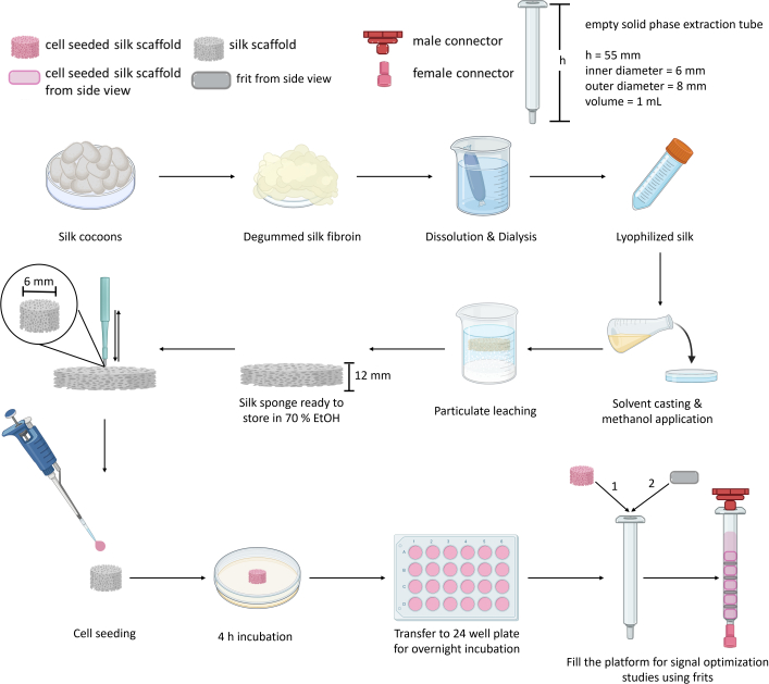
Figure 1: Schematic protocol overview. The flowchart illustrates silk fibroin sponge fabrication, scaffold preparation, and cell seeding, demonstrating step-by-step construction of the signal optimization platform, including cell seeding into the scaffold and the stacking of silk layers and frit components to assemble the final system. Created using BioRender.com. Please click here to view a larger version of this figure.

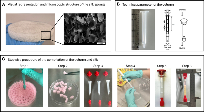
Figure 2: Visual appearance of the produced silk sponge, column, and step-by-step assembling. (A) The produced sponges show a whitish to light yellowish color and are soft and flexible. To provide a more detailed view of the porosity, a scanning electron microscopy (SEM) image was included. The SEM image was taken at a magnification of 50x of the present sponge batch. Scale = 500 µm. The SEM image shows the innumerable pores and their interconnection in combination with their relatively consistent wall thickness. (B) Technical parameters of the column include an overall length of 55 mm, an inner diameter of 6 mm, and an outer diameter of 8 mm. (C) Visual representation of the stepwise assembly of the column. Please click here to view a larger version of this figure.

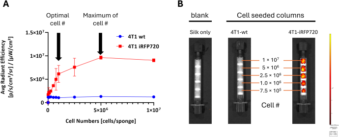
Figure 3: System optimization and assessment of the relationship between signal intensity and cell number. (A) Identification of the ideal cell number on the scaffolds by analyzing the fluorescence images vs cell number. The maximum effective seeding density was determined as 5 × 10⁶ cells/scaffold based on the highest signal intensity without saturation and before signal decrease observed at 1 × 10⁷ cells/scaffold. (B) Epifluorescence images acquired using the in vivo optical imaging analysis software showing fluorescence signal intensity in cell-seeded platforms with increasing cell numbers. Fluorescence intensity increased proportionally with cell number up to 5 × 10⁶ cells/scaffold, after which the signal decreased at 1 × 10⁷ cells/scaffold. Wild-type cell-seeded and blank scaffolds were included as non-fluorescent controls. All experiments were performed in triplicate (n = 3). Error bars represent mean ± standard deviation. Fluorescence signal is reported as average radiant efficiency (p/s/cm²/sr)/(µW/cm²). Please click here to view a larger version of this figure.

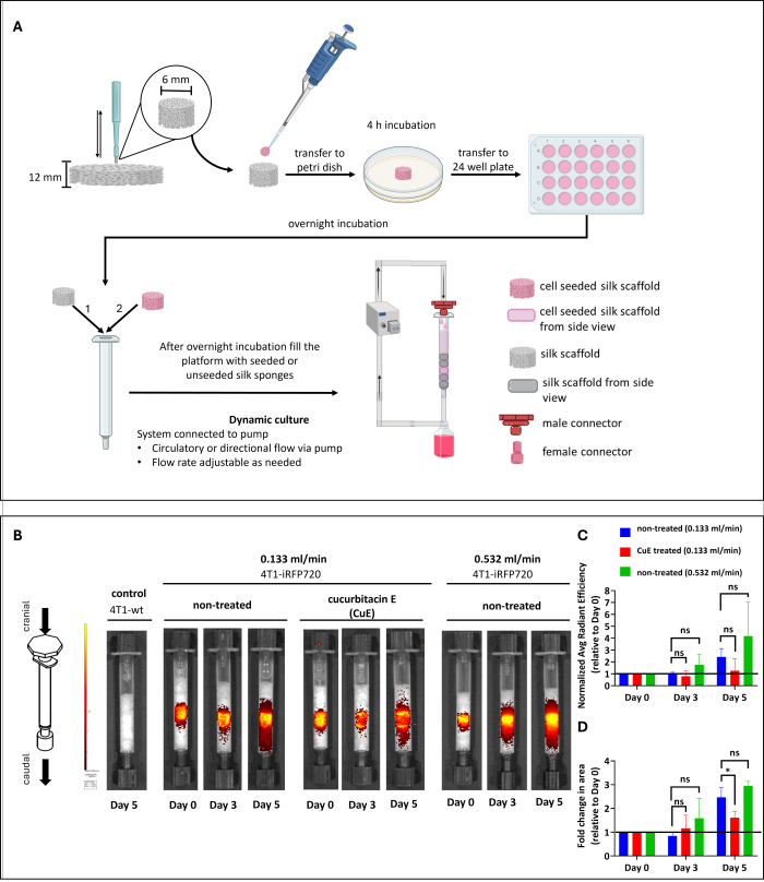
Figure 4: Platform assembly and in vivo optical imaging analysis software-based evaluation of non-treated and treated dynamic culture conditions. (A) Silk fibroin sponges were fabricated and seeded with cells according to the protocol described in Figure 1. For long-term culture experiments, the perfusion system was assembled without frit components. (B) In vivo optical imaging analysis software imaging of 4T1-wt (non-fluorescent control) and 4T1 iRFP720 cells cultured under flow conditions of 0.133 mL/min and 0.532 mL/min flow rates. Non-treated controls were exposed to both flow rates of 0.133 mL/min and 0.532 mL/min. The 0.05 µmol/L Cucurbitacin E (CuE) treated group was only subjected to 0.133 mL/min. Images were acquired over five days using identical settings. (C) Quantification of average radiant intensity from the in vivo images shows a similar signal under both flow conditions compared to Day 0, with no significant difference between the two flow rates. (D) The change fold in area of the migrated cells over time under different flow rate conditions. Normalization was performed to Day 0 values and expressed as fold change relative to baseline. Statistical significance was determined using two-way ANOVA followed by Tukey’s multiple comparison test with α = 0.05; significance levels are indicated in the graphs (*p < 0.05, **p < 0.01, ***p < 0.001, ns - not significant; mean ± standard deviation (SD), n = 3). Panel (A) created using BioRender.com. Please click here to view a larger version of this figure.

Supplementary Figure 1: Software usage steps. (A) Initialize the imaging system. The in vivo Imaging system spectrum CT must be initialized before imaging to ensure that the instrument is properly prepared for image acquisition (red rectangle). (B) Cooling the imaging system. After system initialization, the instrument is ready for use. However, before acquiring an imaging sequence, the system must cool down to -80 °C to ensure stable operating conditions for fluorescence imaging. Once this temperature is reached, the indicator changes from red to green (red arrow). Next, select the optimized settings by clicking Imaging Wizard (red rectangle). (C) Launching the imaging wizard. In the Imaging Wizard, select Fluorescence mode and click Next (red rectangle) to configure the system for fluorescence image acquisition. (D) Selecting the filter pair. Select Filter Pair (red rectangle) and click Next (red rectangle) to proceed, enabling the use of filter settings appropriate for the selected fluorescent probe. (E) Choosing a filter pair in the imaging wizard. A window appears, allowing the selection of filter pairs suitable for the probes and dyes. Choose the appropriate filter pair and click Next to match the imaging setting to the spectral properties of the fluorescent signal. Please click here to download this file.

Supplementary Figure 2: In vivo imaging software Acquisition Control Panel. (A) Removing the pre-selected filter pair. To remove the default filter setting before applying optimized imaging parameters, click Remove > Selected. (B) Setting optimized imaging parameters. Select the optimized parameters to maximize imaging sensitivity and fluorescence signal detections: 1) Set the exposure time to 10 s. 2) Set binning to medium (8). 3) Set F top to 8. 4) Select Excitation Filter 675 nm. 5) Select Emission Filter 720 nm. 6) Click Add. 7) Specify the number of images to be acquired. (C) Performing the final system check before imaging. Before image acquisition, verify that all imaging and saving parameters are correctly configured. 1) Check all settings before starting imaging. 2) Click Acquisition, select Autosave to, and create a folder where the images will be saved. 3) Verify that the device is ready to start (indicated by a green box; red rectangle). 4) To start imaging, click Acquire. Please click here to download this file.

Supplementary Figure 3: Editing image labels. A box Edit Image Labels window will appear. Enter the experimental parameters (e.g., cell count and day of imaging) to ensure proper documentation and identification of each acquired image. Please click here to download this file.

Supplementary Figure 4: Acquiring images. The system acquires images according to the selected parameters, enabling fluorescence signal capture under standardized acquisition conditions. Please click here to download this file.

Supplementary Figure 5: Workflow for Fluorescence Image Analysis and ROI Quantification. (A) Image Analysis. 1) Click File > Browse and select the folder containing the dataset. Then click Open Folder.2) A window containing the dataset will appear 3) Choose the image to be analyzed by double-clicking on it. This step allows the acquired dataset to be opened for subsequent image processing and analysis. (B) Adjusting image display settings. The selected image will appear. 1) Click the Logarithmic Scale box. 2) Uncheck Individual. 3) Select Radiant Efficacy. These settings standardize image visualization and improve fluorescence signal representation. (C) Placing regions of interest (ROIs). Click the box in ROI Tools (indicated by red arrow) and select the required number of ROIs. The selected ROIs will appear. Drag each ROI to the desired location and adjust its shape to match the area of interest for accurate quantification of the selected regions. (D) Measuring ROIs. Click Measure ROIs to quantify the selected regions of interest. (E) Exporting ROIs Data. A box displaying the ROI values will appear. 1) Select Radiant Efficiency. 2) To save the data, click Export, enabling downstream quantitative analysis of fluorescence measurements. Please click here to download this file.

Supplementary Figure 6: Visualization of the female and male components of the system and representative images of background fluorescence. (A) In vivo imaging system images of the empty system and the system filled with silk scaffolds without cell seeding. Images were acquired under different imaging parameters used during system optimization; however, the observed fluorescence behavior remained consistent across conditions. The male connector consistently exhibited autofluorescence, whereas the female connector and the silk-filled system showed no detectable autofluorescence under the imaging conditions used. (B) Female connector. (C–E) Male connector, top, side and bottom view showing the opening. Please click here to download this file.

Supplementary Figure 7: Static groups control images. In vivo imaging system images of non-treated and Cucurbitacin E (CuE)-treated groups under static culture conditions. The images show that signal intensity is comparable at Day 0; however, by the end of the 5-day culture period, the fluorescence signal is no longer reliably quantifiable due to signal loss and reduced detectability due to cell death. Please click here to download this file.

Discussion

The silk sponge production process described in this protocol is standardized, ensuring reproducible scaffold fabrication, as reported in a prior study¹⁶. Production of sponges under fully standardized conditions, such as salt-bed height/amount, silk solution volume, and methanol incubation, is crucial to obtain uniform, comparable sponges. The produced sponges need to follow the quality control protocol criteria published earlier¹⁶. In short terms, the sponge needs to fulfill criteria like a bed height of 12 mm, a pore size between 500–800 µm, a dry weight of a 6 mm diameter sample between 10–15 mg, the absence of a hard top, as well as a uniform porous structure determined using SEM. To standardize the pore size of the sponges, the porogen was sieved using size exclusion meshes according to the European Pharmacopeia, to receive only the fraction between 500–800 µm. For verification, SEM images were processed and the pore size measured using image analysis software according to a previously published paper¹⁶. The volume of the silk solution was optimized to minimize the formation of a hard top and thereby prevent production of unusable sponges¹⁶. Parameters such as salt-bed height can be readily verified by direct measurement, while the silk solution volume can be accurately controlled using a calibrated syringe. Completion of settling of the silk solution in the salt-bed can be observed visually. For a successful methanol incubation, the infiltration time must be considered. A complete infiltration can be detected after the drying steps, showing whitish crystals on top of the sponge. Methanol incubation is particularly important for ensuring scaffold stability. Methanol is reported to induce the beta-sheet formation of the silk protein, making the scaffold water-stable^32,33,16. Because of the application of the salt-bed cast and particulate leaching procedure, the porosity can be adjusted to the desired properties by using different particle sizes of the salt to create different pore sizes, thereby changing the sponge-like structure's properties, e.g., water-holding capacity^34,35. The sponge-like scaffold, with its flexibility and high strength, also allows continuous-flow operation due to its interconnected pores^26,36,37. The seeding of the cells becomes more consistent, resulting in more reliable experimental outcomes, when porosity and sponge height are reproducible.

The 4T1-wt and 4T1-iRFP720 murine breast cancer cell lines were obtained from collaborating partners (co-authors of this study) and have been previously described and characterized¹⁸. Cells should be maintained under the standard culture conditions outlined in the protocol section to preserve stable iRFP720 expression, as any loss of expression can directly compromise imaging results. If the 4T1-iRFP720 cells exhibit reduced iRFP720 expression over time, fluorescence-based cell sorting can be performed to enrich for the positively expressing cell population.

Prior to system signal optimization, the in vivo optical imaging analysis software platform components and silk scaffolds were evaluated to determine whether they produced intrinsic fluorescence that could interfere with the detection of cellular signals. This step was critical to prevent background fluorescence from overlapping with or diminishing the true signal originating from the cells (Supplementary Figure 6A). In addition to its autofluorescence properties, the male Luer-lock contains an opening that facilitates gas exchange (O₂ and CO₂) and enables tubing connections in the dynamic perfusion system. However, this opening also posed a potential contamination risk during imaging; it was replaced with a female Luer-lock, which minimized this risk and improved system sterility during imaging (Supplementary Figure 6B–E). Importantly, because the imaging process is brief, the temporary absence of gas exchange does not adversely affect cell viability. Overall, this modification significantly reduced background autofluorescence, minimized contamination risk, and improved the reliability and accuracy of the software signal detection without compromising cell health or system functionality.

In a prior study, the optimal seeding volume was determined based on the dimensions and absorption capacity of the silk fibroin sponges³¹. Using this optimized configuration, we applied the same seeding strategy in the present protocol and selected 200 µL as the target seeding volume (Figure 4A). This volume represents the maximum amount of cell suspension that can be fully absorbed by the scaffold without overflow, while still providing sufficient nutrients during the initial attachment period. Importantly, this approach allows the total number of cells to be precisely controlled by adjusting the cell concentration within a fixed seeding volume (e.g., 5 × 10⁶ cells/scaffold in 200 µL of medium). The seeding volume is therefore scaffold-dependent and should be adjusted if sponges of different dimensions or porosity are used. Larger or more porous scaffolds may require higher volumes, whereas smaller scaffolds may require proportionally reduced volumes to ensure complete absorption and uniform cell distribution.

Following the optimization of seeding parameters, we proceeded to evaluate the performance of the platform under dynamic culture conditions in absence and presence of a potential metastatic inhibitor, e.g. in this case CuE. Specifically, we established two distinct dynamic perfusion conditions and compared their effects on cell viability, proliferation and migration using in vivo optical imaging analysis software for five days (Figure 4B). To enable quantitative comparison, we used average radiant intensity, a calibrated output of the in vivo optical imaging analysis software system that represents the mean fluorescence signal per pixel normalized to the excitation intensity. This parameter provides a reliable and quantitative measure of fluorophore signal and is directly proportional to the number of labelled cells, making it particularly suitable for longitudinal monitoring of cell populations³⁸. It is important to expose to cells continuously to a media flow, as viability may be reduced under static conditions over time due to limitations in nutrient delivery and waste removal, which are inherent challenges in static 3D culture systems³⁹. Both dynamic perfusion conditions demonstrated a sustained increase in average radiant intensity over time, suggesting improved cell survival and proliferation within the scaffold. The enhanced signal observed under dynamic conditions highlights the beneficial role of perfusion in facilitating nutrient transport, gas exchange, and metabolic waste removal. Radiant efficiency did not differ significantly between treated and control groups, nor between the two different flow rate conditions, suggesting comparable cell numbers (Figure 4C). However, image analysis software-based area analysis indicates altered migration and growth dynamics, with CuE-treated groups showing reduced spreading across the monitored area. Moreover, a higher flow rate (0.532 mL/min) over the 5-day incubation period does not substantially change the overall migrated area compared to the lower flow rate (0.133 mL/min). (Figure 4D). This may indicate that, within the tested range, flow rate does not reach a threshold sufficient to significantly modulate collective cell migration or proliferation. Alternatively, flow-dependent effects may require longer exposure times or higher mechanical stimulation to become detectable in this system^40,41,42.

Optimized 3D culture platforms play a crucial role in studying cell growth and movement under physiologically relevant conditions. Huang et al. demonstrated in a microfluidic platform that interstitial flow modulates cell-cell adhesion and promotes tumor invasion in breast cancer cell models, highlighting the importance of biophysical cues in regulating tumor progression. Goliwas et al. demonstrated the advantages of real-time, longitudinal imaging of cell populations in engineered tumor co-culture systems, enabling improved analysis of dynamic cellular behavior. However, one limitation of this approach is the use of GFP-labelled cells, which have a relatively long half-life (approximately 26 h), potentially leading to signal persistence after cell death and overestimation of viable cell numbers^43,44. In this model, we combined a silk sponge scaffold with iRFP-labelled cells. In contrast to GFP, iRFP fluorescence decreases rapidly upon cell death, enabling more accurate real-time assessment of cell viability, while its near-infrared emission allows improved tissue penetration. The silk sponge scaffold is easy to fabricate and provides more standardized, reproducible results than animal-derived ECM matrices. In addition, it enables continuous perfusion of media through the system, representing a key advantage over conventional hydrogel-based 3D cultures. We systematically optimized each step of the process (from silk scaffold production to cell seeding and imaging) to ensure consistency and reproducibility. From a practical perspective, several factors should be considered to ensure reliable implementation of the protocol. In particular, complete removal of ethanol from the perfusion system is critical and can be achieved by thorough flushing with sterile medium while confirming consistent outlet recovery. Consistency in cell seeding is also important and can be supported by using standardized scaffold dimensions together with pre-optimized seeding volumes and cell numbers³¹. During system assembly, care should be taken to avoid introducing air bubbles and to ensure secure connections, as these may lead to flow instability or leakage. In some cases, weak fluorescence signals may be observed, which can be related to cell health or expression levels; therefore, routine verification prior to seeding and adjustment of imaging parameters may be helpful. Finally, maintaining consistent ROI selection criteria across samples supports reliable image analysis and comparability.

Despite advances in 3D culture systems, 2D models remain the gold standard in drug discovery and development. While multiple factors contribute to this, limited adoption of complex 3D models across laboratories remains a significant barrier. In this work, we aim to address this limitation by providing a simple and accessible approach to establish a dynamic 3D culture platform, thereby facilitating broader adoption of physiologically relevant experimental models. Although the system does not provide single-cell resolution at the microscale, it provides a robust, non-invasive method for quantitative, macroscale assessment of flow-induced collective cell behavior. This approach prioritizes observing population-level growth, spatial redistribution, and movement over individual cell tracking, thereby bridging the gap between simplicity, reproducibility, and biological relevance.

Materials

List of materials used in this article

Name	Company	Catalog Number	Comments
1,1,1,3,3,3-Hexafluoroisopropanol (HFIP)	Sigma-Aldrich	8.04515	Caution: Hazardous. Used for dissolution of freeze-dried silk
24-Well plate	Cellstar, Greiner Bio-One	662102	Storage of cell-seeded scaffolds during incubation
4T1-iRFP720 murine triple-negative breast cancer cells	Macromolecular Cancer Therapeutics Laboratory (MMCT), University of Vienna	N/A	Cell culture experiments; 4T1-iRFP720 was derived in-house from parental 4T1 (ATCC: CRL-2539)
4T1-wt murine triple-negative breast cancer cells	Macromolecular Cancer Therapeutics Laboratory (MMCT), University of Vienna	ATCC: CRL-2539	Cell culture experiments
Bruker Alpha Compact FTIR with Platinum-ATR Sampling Module	Bruker	A220/D-01	FT-IR analysis
Calcium chloride, anhydrous, ≥93% reagent grade	Sigma-Aldrich	902179	For the preparation of dissolution matrix
Cell culture flask, T25	Cellstar, Greiner Bio-One	690175	Consumables; for cell culturing
Cell culture flask, T75	Cellstar, Greiner Bio-One	658175	Consumables; for cell culturing
Centrifuge 5804 R	Eppendorf	5805000010	Used for sample separation by centrifugation
Combi-stopper (female Luer-lock connector)	Braun Melsungen AG	4495101	Used for the platform assembly
Cucurbitacin E	Sigma-Aldrich	SML0577	Cell migration inhibitor
Dermal biopsy puncher, ø 6 mm	Dahlhausen	1190001006	Used to obtain cylindrical sponge scaffolds
Dialysis tubes (3.5 kDa, cellulose)	Spectra/Por by Spectrum Labs	SPEC132724	For dialysis of silk fibroin solution
Dulbecco's Phosphate Buffered Saline	Sigma-Aldrich	D8537	For maintenance of cells
Ethanol, absolute	Merck	1.07017	For the preparation of dissolution matrix
Excel	Microsoft	v2604	Data organization, basic calculations, and plotting
Fetal calf serum (FCS) heat inactivated	Biowest	S181H-500	Supplement for cell culture media
Fiji (former ImageJ)	Open soure (https://imagej.net/software/fiji/)	N/A	Image processing and analysis
GraphPad Prism	GraphPad Software	v8.2.1	Statistical analysis and graph generation
HPLC pump Hitachi L-7120 LaChrom	Merck	K-5244	For dynamic culture conditions in the assembled platform
IVIS 200 Spectrum CT system	PerkinElmer	128201	Optical imaging system with CT capability
IVIS Living Image Software	PerkinElmer	v4.5.2	Software for acquisition, visualization, and quantitative analysis of IVIS imaging data
JEOL JSM-6510 Scanning electron microscope	JEOL GmbH	JSM-6510	SEM images
L-glutamine, 200 mM solution, suitable for cell culture (L-Glu)	Sigma-Aldrich	G7513	Supplement for cell culture media
Lyophilizer Alpha 2-4 LD Plus	Martin Christ	101542	For silk fibroin lyophilization
Male Luer-lock connector	Supelco (Sigma-Aldrich)	57020-U	Adapter for sample reservoirs
Methanol, ≥99.9 %, HPLC Gradient Grade	Carl Roth	7342.1	Caution: Toxic. Induction of beta-sheet formation in silk composites
Optically transparent Solid Phase Extraction (SPE) tubes without frits	Sigma Aldrich	57240-U	Used for the platform assembly
OPUS Spectroscopy software	Bruker	v7.5	FT-IR analysis
Orbital and Linear Shaker MI0103002	Four E'S Scientific	MI0103002	Uniform distribution/mixing
Parafilm PM996	Sigma-Aldrich	P7793	For sealing/wrapping plates and containers for storage (e.g., refrigeration)
Penicillin-Streptomycin, liquid, suitable for cell culture (P/S)	Sigma-Aldrich	P0781	Supplement for cell culture media
Petri dish, 9 cm	VWR	391-0598	For salt-bed sponge casting; for seeding on silk scaffolds
Polyethylene frits for 1 mL SPE tubes	Supelco (Sigma Aldrich)	57244	Used for the platform assembly
RPMI-1640 Medium, suitable for cell culture	Sigma-Aldrich	R0883	Supplemented media is used for silk sponge equilibration, cell culture maintenance and related experiments
Serological pipette, 10 mL	Sarstedt	86.1254.025	Consumables; for maintenance of cells
Serological pipette, 25 mL	Sarstedt	86.1685.020	Consumables; for maintenance of cells
Serological pipette, 5 mL	Sarstedt	86.1253.025	Consumables; for maintenance of cells
Silk cocoons of Bombyx mori L.	Sericulture and Agriculture Experimental Station, Vratsa, Bulgaria	N/A	Raw material for the silk fibroin sponge production
Sodium carbonate, anhydrous, ≥99.5% ACS	VWR	11552.A3	Used for chemical degumming, i.e. removal of sericin
Sodium chloride, ≥98%, technical	VWR	27788.366	For salt-bed sponge casting
SPE Column Push Rod	Carl ROTH	36P9.1	Used for the platform assembly
Stainless steel analytical sieves, 500 µm (ISO 3310-1)	ATECHNIK GmbH	200.050.222-046	For NaCl sieving
Stainless steel analytical sieves, 800 µm (ISO 3310-1)	ATECHNIK GmbH	200.050.222-051	For NaCl sieving
Sterile injectomat line (Tubing), 150 cm, PE	Fresenius Kabi	9004132	Used for dynamic culture conditions
Trypsin - EDTA solution	Sigma-Aldrich	T3924	For maintenance of cells
Ultra-High Performance Centrifuge tubes, 15 mL, sterile	VWR	525-0605	Consumables; for centrifugation, freezing, storage purposes
Ultra-High Performance Centrifuge tubes, 15 mL, unsterile	VWR	525-1083	Consumables; for centrifugation, freezing, storage purposes
Ultra-High Performance Centrifuge tubes, 50 mL, sterile	VWR	525-0609	Consumables; for centrifugation, freezing, storage purposes
Ultra-High Performance Centrifuge tubes, 50 mL, unsterile	VWR	525-1098	Consumables; for centrifugation, freezing, storage purposes
Urine sample cup	Brand	758905	Container for silk solution preparation
Water purification system LaboStar 10 RO DI	Evoqua Water Technologies LLC	W3T324493	Source of ddH2O