Real-Time Assessment of Cut Tobacco Alignment Orderliness Using an Improved Single-Stage Regression Model

Summary

An improved single-stage regression model is developed for real-time detection of cut tobacco alignment orderliness. The approach integrates three structural optimizations and a custom orientation prediction method to enhance detection accuracy while reducing model parameters and computational complexity, enabling efficient assessment of cut tobacco alignment in industrial production environments.

Abstract

Cut tobacco orderliness, defined as the alignment consistency of cut tobacco along the cigarette axis, is a critical factor in production quality optimization. Accurate and automated assessment of this property remains challenging due to complex strand structures and variable imaging conditions. An improved single-stage regression model is developed to enable reliable detection of cut tobacco alignment orderliness. The approach incorporates three architectural modifications: a multifrequency interactive downsampling method to preserve feature information, a triple complementary fusion strategy to enhance multiscale feature representation, and a dynamic detection head to improve localization across different scales. In addition, a custom orientation prediction method is implemented to quantify alignment orderliness. The model is evaluated on an industrial image dataset, achieving a mean average precision of 89.9%, a precision of 90.6%, and a recall of 88.7%. Compared with the baseline model, the proposed approach reduces model parameters by 30.8% (from 2.6M to 1.8M) and computational complexity by 21.5% (from 6.5G to 5.1G), while improving performance. Overall, the method enables efficient and accurate assessment of cut tobacco alignment orderliness and demonstrates suitability for real-time industrial applications.

Introduction

Cut tobacco orderliness refers to the degree of axial alignment of cut tobacco within a cigarette. Understanding the factors that influence this property, such as tobacco morphology and pneumatic conveying parameters, is essential for optimizing the cutting and assembly processes. Consequently, investigating these influencing factors has become a key strategy for tobacco enterprises aiming to reduce costs and improve production efficiency. Traditional assessment of cut tobacco orderliness relies on manual methods, which are inefficient and often lack consistency and accuracy. Therefore, there is an urgent need in the industry for an automated, precise, and real-time detection system to optimize production processes. With the rapid advancement of deep learning, automated evaluation of cut tobacco orderliness based on object detection has become feasible. However, the implementation of such assessment systems on production lines remains a largely unexplored research topic. Nevertheless, machine vision technology has been successfully applied to inspection tasks in other fields¹, providing valuable references for this study. In this context, convolutional neural network (CNN)-based detectors have emerged as the dominant paradigm and are generally categorized into two-stage approaches, such as Faster R-CNN², and single-stage frameworks, such as the You Only Look Once (YOLO) series^3,4.

In recent years, deep learning-based object detection algorithms, particularly the Faster R-CNN framework, have demonstrated significant potential across various domains. However, their direct application to specific industrial and professional scenarios is often constrained by complex operational environments and unique task requirements. Consequently, numerous tailored improvements have been proposed to address these challenges. In medical image analysis, for instance, Su et al.⁵ focused on optimizing parameters and refining network architectures to enhance the detection accuracy of small, critical targets in lung nodule detection. In industrial defect detection, Chen et al.⁶ addressed texture interference in fabric inspection by integrating Gabor filters—optimized via genetic algorithms—into the Faster R-CNN backbone to effectively suppress complex backgrounds. To overcome the challenges of data scarcity and environmental complexity in underwater target detection, Zeng et al.⁷ introduced an adversarial occlusion network. This network competes with the detector during training, compelling the model to learn more robust features and thereby mitigating overfitting. Furthermore, for fine-grained retrieval tasks such as specific instance identification, Li et al.⁸ enhanced Faster R-CNN through feature layer concatenation and fine-tuning strategies, significantly improving its performance on low-resolution images. Wang et al.⁹ recently proposed a multiparty privacy-preserving Faster R-CNN framework that enables secure computation on encrypted images and model parameters through novel protocols for secure division, exponentiation, and logarithm. Sun et al.¹⁰ demonstrated the efficacy of an improved Faster R-CNN in recognizing multiple defect types on wheel hubs, achieving a higher mean average precision (mAP) than R-CNN and YOLOv3. Together, these efforts underscore the continued evolution of Faster R-CNN toward greater adaptability, robustness, and applicability across diverse real-world scenarios. In parallel with these advances in two-stage detectors, single-stage frameworks such as the YOLO series have also undergone substantial development.

As a prominent alternative to two-stage detectors, the YOLO series has gained significant recognition in both industrial and research communities due to its efficient architecture and excellent real-time detection performance. Since the introduction of the first-generation model by Redmon et al.¹¹in 2016, successive iterations have progressively addressed various technical limitations, prompting researchers to develop specialized adaptations for domain-specific applications. In traffic monitoring systems, for instance, Jamtsho et al.¹² implemented YOLOv2 combined with a centroid tracking algorithm to accurately identify license plates of non-helmeted motorcyclists in video streams, effectively reducing false positives while maintaining a high detection rate of 98.52%. For challenging underwater environments, Neelamegam et al.¹³ developed a YOLO-Transformer hybrid model that integrates YOLO’s real-time detection capability with transformer-based attention mechanisms for enhanced contextual understanding. By incorporating real-time IoT sensor data on environmental factors such as turbidity and light levels, the model dynamically adapts to changing conditions, achieving a detection accuracy of 97.5% and outperforming conventional models in noisy, low-visibility scenarios. Similarly, Zhang et al.¹⁴ proposed an improved YOLO model for remote sensing applications. To address challenges of insufficient feature representation and background confusion, they introduced specialized modules for feature enhancement, multiscale fusion, and global context awareness, which significantly improve small object detection accuracy. Collectively, these studies demonstrate the continued evolution of the YOLO series toward greater adaptability, robustness, and effectiveness across diverse real-world scenarios.

Despite these advancements, recent versions of the YOLO family, such as YOLOv11³, are not inherently optimized for the specific textural and structural complexities of cut tobacco in industrial settings. Their standard downsampling operations can lead to the loss of fine-grained features that are crucial for distinguishing aligned from disordered cut tobacco. Furthermore, their fixed-scale detection heads struggle to effectively handle the multiscale nature of tobacco features under varying imaging conditions.

To address these challenges, this paper proposes an improved single-stage regression model based on YOLOv11n, combined with a custom orientation prediction method, for robust online detection of cut tobacco orderliness. The main contributions of this paper are threefold. (1) A multifrequency interactive downsampling (MFID) method is proposed. Standard strided convolution or pooling operations discard fine-grained information, whereas MFID explicitly decomposes features into low- and high-frequency components using the Haar wavelet transform. This approach preserves more original information and mitigates information loss during downsampling. (2) A triple complementary fusion (TCF) method is designed to enhance feature quality by fusing shallow, middle, and deep semantic information. Although simple concatenation or addition operations are commonly used for feature fusion, TCF introduces a middle-layer-guided weighted fusion with inverse weight branches, thereby achieving complementarity between semantic and detailed information. (3) A dynamic detection head (DynamicHead) is introduced to replace the original detection head. The original detection head relies on fixed-scale convolution operations; in contrast, DynamicHead integrates scale-aware, spatial-aware, and task-aware attention mechanisms. This enables dynamic adjustment of feature importance and more flexible and effective multiscale feature fusion, thereby improving the model’s ability to accurately localize and classify orderliness-related features.

Protocol

This study did not involve human subjects, vertebrate animals, or regulated tissues; therefore, no ethical approval or institutional review board approval was required. The dataset used in this study was obtained from Longyan Tobacco Industry Co., Ltd. Images were collected from five independent production batches over a three-month period. Sampling was performed randomly at different times of day (morning, afternoon, and night) to capture natural variations in production conditions. The dataset includes samples covering a tobacco moisture range of 12%–18%, cutting speeds of 1.5, 2.0, and 2.5 m/s, and pneumatic conveying pressures of 0.4, 0.5, and 0.6 MPa, thereby ensuring coverage of typical production conditions.

Dataset Acquisition and Setup
Hardware configuration
The image acquisition system was configured to meet the requirements for detecting the orderliness of cut tobacco in heat-not-burn cigarettes. It mainly consisted of an industrial camera, an industrial lens, a vision light source, and an industrial control unit. The system employed an MV-CH120-10GC industrial camera paired with an MVL-KF0818M-12MP industrial lens to capture high-definition images of the cut tobacco region on the surface of sectioned cigarette rods. The camera was positioned at a working distance of 150 mm from the cigarette rod surface. The strip LED light source was mounted coaxially with the camera at a distance of 80 mm from the target, with an incident angle of 45°. Imaging was performed inside a matte-black enclosure to eliminate ambient light interference. The enclosure is a matte-black painted aluminum hood with internal dimensions of 400 mm (width) × 350 mm (depth) × 300 mm (height), and interior surfaces coated with matte-black paint (reflectance < 5% at 550 nm) to minimize internal reflections and ensure consistent lighting conditions. To ensure imaging quality and consistency, an MV-LRDS-H-95-30-W light source was used to establish a stable illumination environment, minimizing the impact of ambient light variations on tobacco strand contour extraction and orientation recognition. The acquired images were received, processed, and stored by a PC1010-AX360 industrial computer, which also performed subsequent recognition algorithms, result computation, and interface output. No explicit camera calibration or distortion correction was performed, as the industrial camera and lens combination exhibited negligible radial distortion (less than 0.5% at the image edges) within the field of view of 896 × 1600 pixels. The camera and light source were rigidly mounted on a fixed frame to ensure positional stability during image acquisition. The light source intensity was maintained at a constant level throughout image acquisition. The field of view was configured to fully cover the exposed cut tobacco region within the steel support structure.

Camera parameter setting
Image acquisition was triggered, and images were captured after the sample cigarette was positioned and sectioned and then saved in JPG format. To ensure consistency of the acquired images, the acquisition parameters were manually set. Specifically, the image resolution was set to 896 × 1600. The exposure time was initially set to 4000 µs and could be fine-tuned within a range of 3000 to 6000 µs according to on-site brightness. All parameter tuning was performed with the sample placed inside the matte-black enclosure described above, under fully controlled lighting conditions. No external ambient light was present during tuning, as the imaging system operated within a fully enclosed environment with room lights turned off. The gain was initially set to 2 dB and controlled within a range of 0 to 6 dB based on noise levels. The gamma value was set to 0.8, and the white balance was configured with fixed parameters. The final acquisition parameters were set as follows: exposure time = 4000 µs, gain = 2 dB, gamma = 0.8, white balance mode = fixed, image resolution = 896 × 1600 pixels, and image format = JPG. For white balance, the fixed-parameter mode was used. Calibration was performed using a standard white reference card (X-Rite ColorChecker) placed at the sample position. The red and blue channel gains were adjusted until the RGB values of the white card were equalized within a ±2% deviation. After calibration, the white balance parameters were fixed as follows: red gain = 1.2, green gain = 1.0 (fixed), and blue gain = 1.5. Calibration was performed once after each system startup or whenever the light source showed signs of aging that could cause color temperature drift. These settings helped ensure clear boundaries of cut tobacco and stable brightness distribution while also meeting the processing requirements for subsequent tobacco strand segmentation, orientation calculation, and orderliness analysis.

Image collection
Image acquisition targeted the cut tobacco area exposed on the surface of heat-not-burn cigarette rods after sectioning. During detection, the cigarette sample was first delivered to the inspection station, where its posture and position were adjusted and fixed by the sample positioning mechanism. The positioning mechanism consists of a pneumatic clamp with V-shaped alignment guides. The system achieves a positional repeatability of ±0.5 mm over 1000 consecutive cycles, as verified by laser displacement sensor measurements. Subsequently, the outer wrapping material was stably sectioned by the cutting mechanism, fully exposing the surface cut tobacco within the field of view of the vision system. A circular rotating blade (diameter 50 mm, thickness 0.3 mm, material high-speed steel) was used. Cutting depth was set to 1.5 mm with a rotational speed of 300 rpm. Cutting consistency was monitored by linear encoder feedback, maintaining thickness variation within ±0.05 mm. Once the sample position was stable and the imaging region was clearly defined, image acquisition was performed using the industrial camera under stable illumination provided by the light source. A total of 634 images were collected; typical images are shown in Figure 1. The dataset includes three tobacco density levels (low, medium, high; approximately 180, 220, and 260 mg/cm³), strand orientations spanning −180° to 180°, and lighting conditions ranging from normal lighting to low-light edge conditions. Illuminance was measured using a calibrated digital lux meter (TA8133, accuracy ±3%) with the sensor positioned at the sample surface location. The measured normal lighting range is 200–800 lux, provided by the strip LED light source within the enclosed hood, with no ambient light leakage. The low-end value (approximately 200 lux) represents an edge-case condition created by dimming the light source to evaluate model robustness. In addition, partial occlusion of tobacco strands (ranging from 10% to 50%) is present in approximately 30% of the images. These variations reflect real production line diversity.

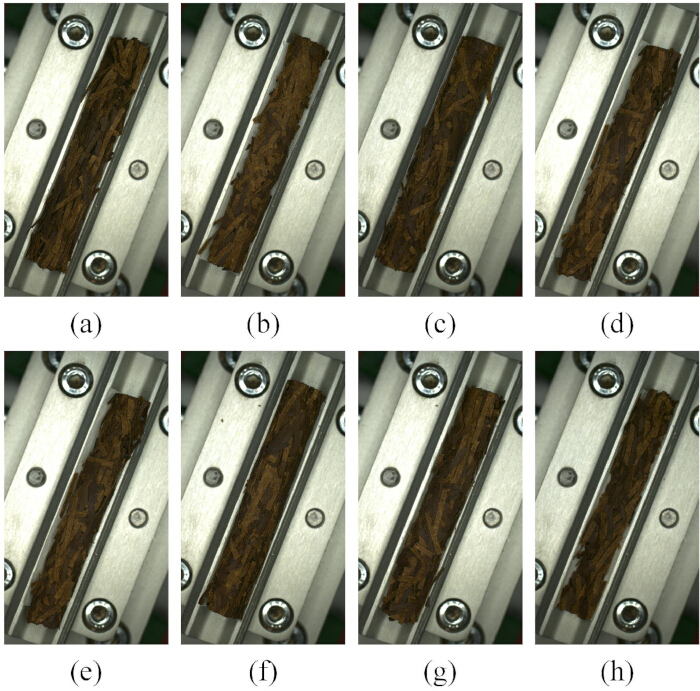
Figure 1. Representative raw images of cut tobacco acquired by the vision system. (a–h) Representative examples of raw images of cut tobacco captured under industrial field conditions using the image acquisition system. Images were obtained at a resolution of 896 × 1600 pixels under controlled illumination using a strip light source to ensure uniform brightness and minimize environmental interference. These images illustrate variations in tobacco strand distribution, density, and orientation prior to model processing. Please click here to view a larger version of this figure.

Image annotation
Using the open-source tool LabelImg, bounding boxes were drawn around visible cut tobacco and steel support features. The correct angle was assigned as the label for each bounding box. The horizontal axis (0°) was defined as the rightward direction parallel to the image bottom edge. For each tobacco strand, the annotation tool’s angle measurement function was used to draw a line along the strand’s major axis. The angle was recorded as the angle between this axis and the horizontal reference (range: −180° to 180°). Annotations were saved in the standard single-stage detection format, with one TXT file corresponding to each image. Each .txt file contains lines formatted as: class_id x_center y_center width height. Coordinates are normalized to [0,1] relative to image dimensions. Class 0 = tobacco strand, class 1 = steel support. The angle label is stored as a sixth column in the annotation .txt file, appended after the five standard YOLO fields. The exact format per line is: class_id x_center y_center width height angle. The angle value is stored in degrees as a floating-point number ranging from −180.0 to 180.0, with two decimal places (e.g., 45.75). Example line: 0 0.5230 0.4170 0.0850 0.0620 38.25.

Quality control
A second annotator reviewed a randomly selected 20% of the annotated images. Random selection was performed using the random.sample() function from the Python random library with a fixed random seed of 2024. A list of all image filenames was generated, and 20% of the images were sampled without replacement using this seeded random number generator, ensuring reproducible selection across repeated quality control procedures. Any discrepancies were discussed and resolved, ensuring labeling consistency. Inter-annotator agreement was assessed using angular deviation: the mean absolute difference between the two annotators’ angle labels was 2.8° (standard deviation = 1.5°). Annotations with deviation >5° were reviewed and reconciled.

Single-Stage Regression Model for Cut Tobacco Orderliness Detection
The detection of cut tobacco alignment orderliness is crucial for improving both the manufacturing process and the final product quality in cigarette production. However, this inspection task faces several challenges, including overlapping cut tobacco, small target sizes, and uneven illumination, all of which compromise detection accuracy and robustness. An improved single-stage regression model based on YOLOv11n is used for the online detection of cut tobacco orderliness. The proposed framework accurately identifies the morphological features of cut tobacco during cigarette rod formation, enabling reliable detection of alignment regularity while improving accuracy, robustness, and real-time processing capability. The overall configuration of the proposed single-stage regression framework is shown in Figure 2.

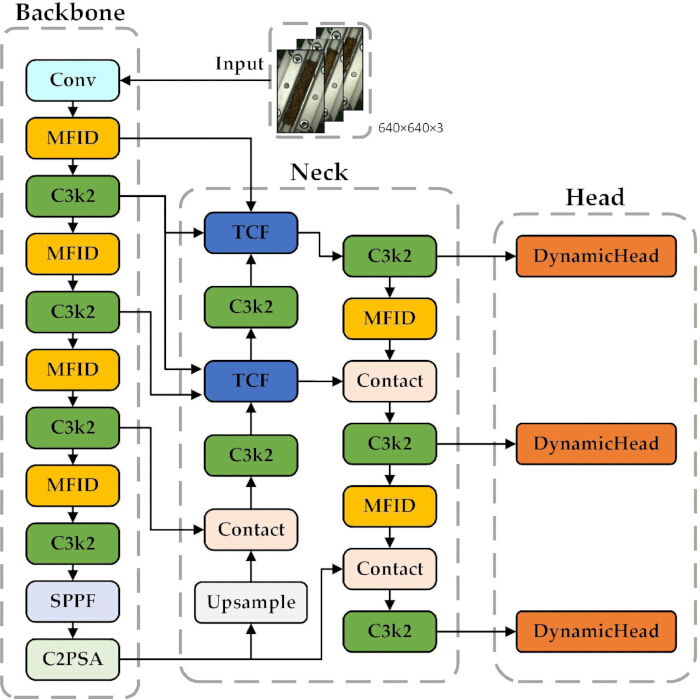
Figure 2. Overall architecture of the proposed single-stage regression model. The diagram illustrates the complete network structure, including the backbone, neck, and detection head. The backbone extracts multiscale features, incorporating multifrequency interactive downsampling (MFID) modules to preserve feature information. The neck integrates features using the triple complementary fusion (TCF) strategy for enhanced multilevel representation. The detection head adopts the DynamicHead module, which integrates scale-aware (π_L), spatial-aware (π_S), and task-aware (π_C) attention mechanisms to improve localization and classification performance. Please click here to view a larger version of this figure.

Multifrequency Information Downsampling Module (MFID)
In the backbone network of YOLOv11, the convolutional operation with a stride of 2 performs downsampling by skipping pixels. This process directly discards half of the spatial information, resulting in the loss of high-frequency details (e.g., edges and textures of small objects) and significant information loss for small targets. Furthermore, the max-pooling and average-pooling operations in the backbone also discard detailed information within object regions, smooth features, and introduce noise, all of which negatively affect feature learning.

To address these issues, an MFID module is introduced, inspired by the concept of wavelet hierarchical decomposition^15,16. This module first decomposes features into two complementary parts using the Haar wavelet transform: low-frequency background information, which enhances classification, and high-frequency details rich in edges and textures, which improve small-target detection. To further strengthen the perception of small targets, the MFID module incorporates two additional branches: a max-pooling branch that leverages translation invariance to preserve fine-grained features of small targets, and a strided-convolution branch that utilizes learnable parameters to achieve stronger representational capacity and richer information composition. Through this multibranch structure, the MFID module preserves more complete spatial and frequency information during downsampling. The architecture of the MFID module is illustrated in Figure 3.

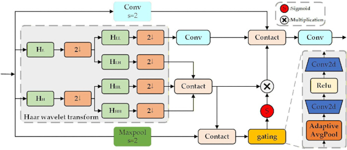
Figure 3. Structure of the MFID module. The MFID module separates input features into low-frequency and high-frequency components using a Haar wavelet transform to preserve critical structural information during downsampling. H_LL denotes the low-frequency approximation component, while H_LH, H_HL, and H_HH represent high-frequency detail components in the horizontal, vertical, and diagonal directions, respectively. The symbol 2↓ indicates two-fold downsampling. Feature maps from multiple branches are fused through concatenation and gating mechanisms to enhance feature representation. Please click here to view a larger version of this figure.

During downsampling, the image is decomposed using the Haar wavelet transform, which is adopted for its simplicity and efficiency in decomposing low- and high-frequency features, making it suitable for real-time detection tasks. H_L and H_H denote the low-pass and high-pass decomposition filters, respectively, and are employed to extract low-frequency and high-frequency information from the image. The wavelet basis function and scaling function for a one-level, one-dimensional Haar transform are defined using Equation 1 as follows:

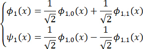(1)

The Haar basis function is defined using Equation 2 as follows:

(2)

Here, parameters j and k denote the scaling coefficient and translation amount of the Haar basis function, respectively. Specifically, the zero-order Haar basis function is defined using Equation 3 as follows:

(3)

In Figure 3, the symbol 2↓ denotes two-fold downsampling. A two-level Haar wavelet decomposition yields four components: the low-frequency approximation (H_LL) and the high-frequency detail components in the horizontal (H_LH), vertical (H_HL), and diagonal (H_HH) directions. The H_LL component carries contour, background, and global information, whereas the high-frequency components (H_LH, H_HL, and H_HH) capture edge, texture, and fine-grained features.

The high-frequency components H_LH, H_HL, and H_HH obtained after two-fold downsampling are concatenated by the Concat operation, thereby integrating the multidirectional detailed information to generate the integrated high-frequency detail information , as shown in Equation 4.

(4)

Subsequently, secondary information fusion is performed on the max-pooling branch to integrate detailed features with global features, thus generating reconstructed information , as shown in Equation 5, which incorporates a broader set of salient features and reutilizes high-frequency detailed information for enhanced feature representation.

(5)

Thereafter, a gating mechanism is employed to dynamically regulate information flow, and the  is leveraged to guide the identification of small target features within the , preserving useful features while suppressing inherent useless noise interference. The gating mechanism is defined as: gating(x) = Linear_2(ReLU(Linear_1(x))), where Linear_1 reduces the channel dimension by a reduction factor of 4, and Linear_2 restores it to the original channel dimension. The output of the gating mechanism is passed through a Sigmoid activation to produce modulation weights in the range [0,1]. The learnable parameters include the weight matrices and bias terms of both Linear layers, which are initialized using uniform initialization. This ensures that detailed and critical feature information is properly balanced and utilized, yielding final detailed feature  as presented in Equation 6.

(6)

Finally, the stride-convolution downsampling information, low-frequency vector, and final detailed feature are concatenated via Concat to expand the feature downsampling interaction across multiple dimensions and frequency bands, as shown in Equation 7.

(7)

Action-implementation steps
Module definition
A custom PyTorch module named MFID should be defined within the project’s model definition files. The implementation of this module consists of four parallel paths: (1) Wavelet transform: a two-level decomposition is applied to the input feature map using predefined Haar wavelet filters, generating a low-frequency approximation component and high-frequency detail components in the horizontal, vertical, and diagonal directions, after which the three high-frequency components are concatenated; (2) Max-pooling: max-pooling is applied to the input to preserve salient features; (3) Strided convolution: standard downsampling is performed through a convolutional layer with a stride of 2; (4) Feature reconstruction and fusion: first, the high-frequency information obtained from the wavelet transform is fused with the features from the max-pooling branch; subsequently, a gating mechanism guided by the low-frequency information is employed to filter fine-grained features; finally, the processed fine-grained features, low-frequency components, and strided convolution output are concatenated to obtain the final downsampled feature map.

Configuration file editing
The baseline model configuration file (config.yaml) should be opened. All instances of standard downsampling modules in both the backbone and neck networks should be systematically identified. Each identified downsampling module entry should then be replaced with the MFID module.

Design motivation
The MFID module is designed to mitigate information loss in standard downsampling operations, which is particularly detrimental to small object detection. Its core concept is inspired by wavelet hierarchical decomposition. By explicitly separating low-frequency global information from high-frequency detail information in the image and processing them accordingly, the module ensures that critical texture and edge features are preserved during downsampling. The incorporation of max-pooling and strided-convolution branches further captures and supplements features from complementary perspectives—specifically, translation invariance versus learnable representation. Through multibranch fusion, the module provides subsequent network layers with a more informative and robust multifrequency feature representation. All unspecified architectural parameters and layer configurations follow the default implementation settings of the YOLOv11n framework within PyTorch.

Triple-Cross Feature Fusion Module (TCF)
At the neck feature fusion stage of the YOLOv11 network architecture, a simple concatenation operation is typically used to merge feature maps of the same scale. However, this direct approach has clear limitations: first, it fails to fully account for semantic differences among features at different levels; second, the lack of explicit modeling of inter-channel correlations makes small-target features prone to dilution or loss during fusion, thereby compromising detection performance. To address these issues, a more interactive fusion method, termed the TCF module, is introduced¹⁷. This method employs a multilevel progressive fusion strategy that guides information flow toward small-target detection through cross-layer transmission. It also incorporates additional nonlinear operations to explore deep-level information across scales, thereby enhancing the fusion of multiscale features. Unlike conventional modules that rely on simple addition or average fusion, TCF adopts a weighted fusion approach. This allows it to adaptively learn detailed information at each level, dynamically optimize information extraction pathways, and focus on the most discriminative features, ultimately improving detection accuracy. The architecture of the TCF module is illustrated in Figure 4.

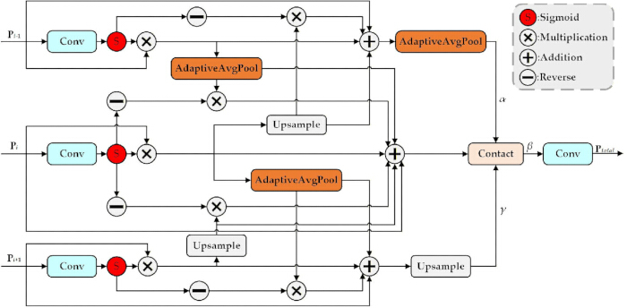
Figure 4. Structure of the TCF module. The TCF module performs multilevel feature fusion across shallow, middle, and deep layers to improve representation of small targets. P represents input feature maps at different levels. Conv denotes convolution operations, Upsample indicates feature upsampling, and AdaptiveAvgPool represents adaptive average pooling. The module integrates calibrated features through weighted fusion and cross-layer interaction to enhance semantic and spatial feature complementarity. Please click here to view a larger version of this figure.

In the task of object detection, the information contained in deep-layer feature P_i+1 and shallow-layer feature P_i-1 differs significantly. To enhance the fusion of cross-layer information, middle-layer P_i is introduced as the final feature fusion layer to balance the differences among feature information across different levels.

First, the input information of the shallow, middle, and deep layers is processed using the Sigmoid activation function to generate weighted features , , and , which serve to strengthen key features and weaken redundant ones, as shown in Equation 8.

(8)

Second, the input information of the shallow, middle, and deep layers is multiplied element-wise by the mapped weighted features to generate calibrated features , , and , as shown in Equation 9. The importance of features is dynamically adjusted via the weight attention mechanism, thus achieving adaptive feature selection and recalibration.

(9)

At the middle-layer feature fusion stage, two inverse weight branches are leveraged to fuse with the calibrated shallow-layer and deep-layer features, respectively, filtering out the false detailed information induced by noise in the shallow-layer features and the biased associated semantic information in the deep-layer features. Subsequently, the multibranch information is integrated, and the original features, calibrated features, and interactive features of this layer, as well as the calibrated shallow-layer and deep-layer features, are fused together. This achieves the preservation and complementation of multiscale feature information, mitigates the issues of small-target information loss and misjudgment, and finally yields middle-layer fused features , which are formulated using Equation 10 as follows:

(10)

The associations between the shallow layer, deep layer, and middle layer are established separately, as shown in Equations 11 and 12.

(11)

(12)

Finally, the outputs of the three feature fusion paths are concatenated via the Concat operation to preserve the feature independence of each individual path. Key information from each path is dynamically learned based on the weights α, β, and γ, which are defined as learnable scalar parameters initialized to 1.0 and optimized via backpropagation during training, enabling dynamic balancing of contributions from shallow, middle, and deep feature paths. Furthermore, convolutional operations are employed to aggregate contextual information, eliminate incoherent feature boundary responses caused by cross-layer concatenation, and optimize the acquisition and refined representation of small-target detailed information. The process is formulated using Equation 13 as follows:

(13)

Action-implementation steps
Module definition
A custom PyTorch module named TCF should be defined within the project’s model definition files. This module takes as input the shallow-layer, middle-layer, and deep-layer feature maps extracted from different stages of the backbone network. Its internal processing flow consists of three main steps: (1) Feature calibration: the Sigmoid function is applied to each of the three input feature layers to generate weight maps, which are then multiplied element-wise with the original feature maps to enhance key features while suppressing redundant ones; (2) Interactive fusion: at the middle-layer feature fusion stage, two inverse weight branches are introduced to fuse with the calibrated shallow-layer and deep-layer features, respectively, filtering out false detailed information induced by noise in the shallow-layer features and biased associated semantic information in the deep-layer features; (3) Multipath aggregation: the original features, calibrated features, interactive features, and features fused with shallow and deep information are integrated, after which convolutional operations are applied to eliminate incoherent feature boundary responses caused by cross-layer concatenation, ultimately outputting fused features rich in multiscale information.

Configuration file editing
The model configuration file (config.yaml) should be opened. The feature fusion sections in the neck network—specifically, the layers where features from different stages of the backbone network are fused—should be located. At these positions, the original simple concatenation operation layers should be replaced with a call to the TCF module, ensuring that the module inputs are correctly connected to the corresponding shallow, middle, and deep features.

Design motivation
The design of the TCF module is motivated by the challenges of information disparity and information loss during feature fusion. Shallow features are rich in detail but contain considerable noise, whereas deep features exhibit strong semantics but low resolution. To address this, the TCF module introduces a middle-layer feature as an information balancer and incorporates carefully designed calibration, interaction, and aggregation pathways to maximize the complementary advantages of cross-level features. The underlying motivation is to establish a more effective fusion mechanism capable of dynamically evaluating the importance of features at each level and selectively integrating information. As a result, it generates a high-quality feature representation for the subsequent detection head that is rich in both detail and semantic information, making it particularly suitable for small object recognition.

DynamicHead Module
The detection head component serves the fundamental purpose of performing multiscale object recognition on feature representations generated by the backbone and feature fusion networks. This process enables accurate spatial localization of detected objects, categorical assignment, and reliability estimation of bounding box predictions. Given the substantial scale variations of target features in visual data and the dense concentration of bounding box proposals in certain frames, precise cut tobacco identification requires the analysis of multiscale patterns. To address this, the method adopts the DynamicHead architecture¹⁸ as a replacement for the native detection head in YOLOv11n, establishing a self-attention framework that integrates scale-aware, spatial-aware, and task-aware mechanisms to enhance both detection capability and operational efficiency. The structural configuration of the DynamicHead component is illustrated in Figure 5.

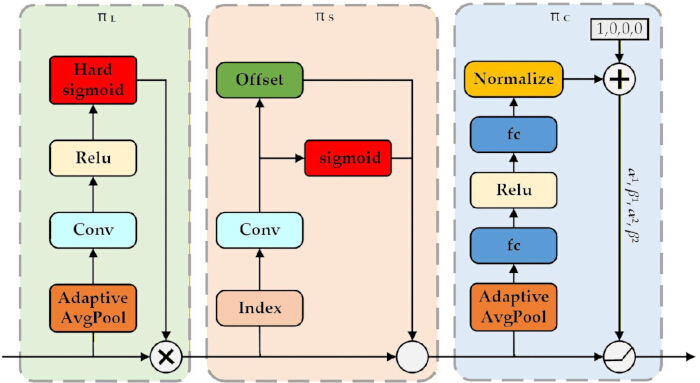
Figure 5. Structure of the DynamicHead detection module. The DynamicHead module incorporates three sequential attention mechanisms: scale-aware (π_L), spatial-aware (π_S), and task-aware (π_C). These components dynamically adjust feature importance across scales, spatial regions, and detection tasks. This design improves both localization accuracy and classification performance by enabling adaptive feature refinement within the detection head. Please click here to view a larger version of this figure.

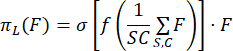
This architecture comprises three specialized attention units: scale-aware (π_L), spatial-aware (π_S), and task-aware (π_C) components. The scale-aware attention mechanism (π_L) first averages the input feature map across spatial and channel dimensions. The result is passed through a linear projection layer followed by a hard-sigmoid activation to generate scale weights, which are then multiplied element-wise with the original feature map. The spatial-aware attention mechanism (π_S) employs deformable convolution with K = 9 sparsely selected sampling points. It predicts offset vectors Δpk and modulation scalars Δm_k for each sampling point, then aggregates the sampled features to produce spatial attention weights. The task-aware attention mechanism (πC) applies a learnable linear transformation to each channel independently using two sets of parameters (α¹, β¹ and α², β²). It selects the maximum response between the two transformed representations to dynamically adapt features for classification and regression tasks. Finally, these three attention mechanisms are applied sequentially to the input feature map as F_out = πC(πS(πL(F) · F) · F) · F. The scale-aware mechanism employs cross-scale feature weighting to adaptively combine multiresolution representations, thereby refining model sensitivity to dimensional variations. The spatial-aware component implements regional emphasis weighting within feature mappings, directing computational focus toward foreground entities while suppressing irrelevant background interference. Meanwhile, the task-aware module dynamically modulates output representations for specific objectives, refining both classification and regression outcomes to strengthen model precision and operational robustness. The computational procedure is formalized in Equations 14–17.

(14)

(15)

(16)

(17)

Here, W_L(F) denotes the attention-enriched feature representation, while π_L(F), π_S(F), and π_C(F) correspond to scale-, spatial-, and task-oriented attention operations, respectively. The transformation f represents a linear projection layer, σ(x) indicates hard-sigmoid activation processing, K specifies the quantity of sparsely selected spatial points, p_k+Δp_k introduces positional adjustments to emphasize discriminative areas, Δm_k constitutes a trainable significance measure for spatial point p_k, and α(F) and β(F) are learnable parametric functions governing activation thresholds. Among them, K is set to 9 in all experiments, as this value provides sufficient spatial coverage while maintaining computational efficiency.

Action-implementation steps
Module definition
A custom PyTorch module named DynamicHead should be defined within the project’s model definition files. The implementation of this module consists of three attention units applied sequentially: (1) Scale-aware attention: feature layers at different scales are dynamically weighted using learnable parameters; (2) Spatial-aware attention: based on the concept of deformable convolution, this unit focuses on sparse yet discriminative spatial locations within the feature maps; (3) Task-aware attention: activation thresholds are dynamically learned to optimize feature representations for classification and regression tasks, respectively. These three attention mechanisms are sequentially applied to the input feature pyramid, ultimately producing features for prediction. All modules were implemented using standard PyTorch operations, including convolutional layers, linear layers, activation functions, and attention mechanisms as described above.

Configuration file editing
The model configuration file (config.yaml) should be opened. The section defining the detection head should be located. The original detection head configuration, which typically comprises a series of convolutional layers for classification and regression, should be replaced with a call to the DynamicHead module, ensuring that its input is connected to the feature pyramid output by the neck network.

Design motivation
Traditional detection heads typically apply the same set of convolutional parameters to all feature layers, spatial locations, and tasks, lacking task-specific adaptability. The introduction of the DynamicHead module is motivated by the complexity of detection tasks, aiming to decouple and address these challenges through a unified attention-based architecture. Its design motivation is threefold: (1) to adaptively focus on feature layers corresponding to targets of different sizes via the scale-aware module; (2) to concentrate computational resources on foreground target regions rather than background via the spatial-aware module; and (3) to dynamically optimize feature representations for the distinct objectives of classification and regression via the task-aware module. This combination of decoupling and dynamic optimization enhances the model’s localization accuracy and classification reliability for densely arranged, multiscale targets such as cut tobacco.

Custom Assessment Method for Cut Tobacco Orderliness
Module description and design principle: The quantitative evaluation of cut tobacco alignment orderliness is essential for assessing manufacturing process stability and predicting final product quality in cigarette production. Traditional assessment methods rely on manual visual inspection, which is subjective, time-consuming, and unable to provide consistent quantitative measurements. To address these limitations, a custom angle prediction method integrated with the improved single-stage regression detector is used. The fundamental principle of this method is to establish a spatial reference framework using the steel support structure within the cigarette rod as a geometric benchmark. Because the steel support maintains a fixed orientation during manufacturing, it serves as an ideal reference line for calculating the relative orientation of individual cut tobacco. By measuring the absolute angles of detected cut tobacco and the steel support relative to the horizontal reference line and subsequently computing their relative angular differences, the method provides a quantitative assessment of alignment orderliness. A relative angle of zero indicates perfect parallelism between a strand and the support, whereas increasing angular deviation signifies poorer alignment. The horizontal reference axis is defined as the line parallel to the bottom edge of the image, oriented from left to right. This axis corresponds to 0°, with positive angles measured counterclockwise and negative angles measured clockwise from this axis. The final orderliness metric is obtained by averaging the relative angles of all detected strands within an image, enabling consistent and objective quality grading.

Action-implementation steps
Angle calculation module definition
Implement a post-processing module that processes the detection outputs from the improved single-stage regression model. For each detected object (cut tobacco and steel support), extract the bounding box coordinates. Calculate the center point coordinates for each detected object using Equation 18. Compute the image center point coordinates based on the image dimensions using Equation 19.

  (18)

   (19)

where x₁, x₂, y₁, y₂ denote the coordinates of the four corners of the detected bounding box for either a tobacco strand or the steel support; c_x and c_y represent the coordinates of their respective center points within the detection region; w and h indicate the width and height of the cigarette image; d_x and d_y define the coordinates of the image center point.

Absolute angle computation
For each detected tobacco strand and the steel support, calculate the vector from the image center to the object center. Compute the absolute angle relative to the horizontal reference line using the arctangent function, as formulated in Equation 20. The angle is computed using atan2(d_y, d_x), where atan2 is the four-quadrant inverse tangent function available in the Python math library. This function returns values in the range (−π, π] radians, which are then converted to degrees, yielding output angles in the range (−180°, 180°]. Quadrant handling is automatic with atan2 based on the signs of d_y and d_x. This yields A_steel for the steel support and A_cut for each tobacco strand.

(20)

Relative angle calculation
For each detected tobacco strand, compute the relative angle by subtracting the steel support’s absolute angle from the strand's absolute angle, as shown in Equation 21. The absolute value ensures positive angular deviation measurements.

(21)

Orderliness metric generation
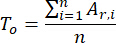
Aggregate the relative angles of all detected strands within a single image. Calculate the average relative angle by summing all relative angles T_o and dividing by the total number of detected strands n, as formulated in Equation 22. This average value serves as the quantitative measure of alignment orderliness for that image.

(22)

Quality grading implementation
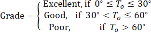
Implement a classification function that maps the calculated value to qualitative grades based on predefined thresholds, as defined in Equation 23. The grading thresholds (0°–30° = Excellent, 30°–60° = Good, >60° = Poor) were established based on consultation with three quality control experts from Longyan Tobacco Industry Co., Ltd. These experts independently evaluated 200 sample images and correlated the calculated average relative angles with perceived alignment quality, using a three-category scale (Excellent, Good, and Poor). The 30° and 60° boundaries were selected as the consensus cutoffs where inter-expert agreement exceeded 90%. This grading enables intuitive interpretation of the quantitative results for quality control personnel.

(23)

Configuration file editing
The model configuration file (config.yaml or model.yaml) should be opened. The post-processing section or the inference settings portion of the configuration should be located. The custom angle calculation module should be properly referenced and enabled. The output parsing settings should be verified to correctly extract bounding box coordinates for both cut tobacco and the steel support. No additional layer insertion is required for this assessment method, as it operates as a post-processing module after the detection head outputs.

Design motivation
The design of this custom assessment method is motivated by the need to transform subjective visual inspection into objective, reproducible quantitative measurements. Traditional manual inspection suffers from inter-observer variability and cannot provide continuous numerical data for process optimization. By leveraging the steel support as a natural geometric reference within the cigarette rod, the method eliminates the need for external calibration markers and ensures measurement consistency across different images and production batches. The use of center-point vectors and arctangent calculations provides a mathematically robust and computationally efficient approach to angle estimation, making it suitable for real-time deployment. This vector-based computation from the image center to the object center is designed to be invariant to camera field of view and the cigarette rod’s position within the image, thereby ensuring robustness under varying capture conditions. The averaging strategy across multiple detected strands accounts for natural variations in strand orientation and yields a statistically reliable overall orderliness metric. A three-tier grading system translates continuous numerical measurements into actionable quality categories, facilitating rapid decision-making in production line quality control. Overall, this integrated approach combines the detection capabilities of the improved single-stage regression model with precise geometric computations, enabling comprehensive and automated assessment of cut tobacco alignment orderliness.

Model Training for Cut Tobacco Orderliness Detection
PyTorch 2.1.0, Compute Unified Device Architecture (CUDA) 12.1, and all dependencies should be properly installed. The implementation follows standard PyTorch YOLO pipelines and can be reproduced based on the detailed module descriptions and configuration steps provided.

Training command
Before retraining, the partitioned image dataset and annotation files in the standard single-stage detection format (e.g., YOLO format with one .txt file per image) should be prepared. A dataset configuration .yaml file specifying the image paths, number of classes (cut tobacco and steel support), and class names should be created. Based on the model improvements described previously, the original detector .yaml configuration file should be replaced with the proposed model .yaml file, which incorporates the MFID, TCF, and DynamicHead modules. The train.py script should be written or modified to import the single-stage detector package, load the training model and dataset configuration, and set the following training parameters: imgsz=640, epochs=100, batch=4, workers=0, device='0', optimizer='SGD', close_mosaic=10, etc. The random seed was fixed to 42, and model weights were initialized using the default initialization strategy provided by the deep learning framework. Reproducibility was ensured by setting torch.backends.cudnn.deterministic = True and torch.backends.cudnn.benchmark = False.

Hyperparameters
The key hyperparameters configured for training are as follows: input image resolution of 896 × 1600 pixels; batch size of 4, constrained by GPU memory; initial learning rate of 0.01 with a cosine annealing scheduler for gradual decay; stochastic gradient descent (SGD) optimizer with momentum of 0.912 to accelerate convergence; and weight decay of 0.0004 for regularization. Images were normalized using mean [0.485, 0.456, 0.406] and standard deviation [0.229, 0.224, 0.225]. Augmentation included random horizontal flip (50%), random brightness adjustment (±20%), and random rotation (±15°). Mosaic augmentation is enabled by default during the early training epochs to enhance model robustness to varying object scales and occlusions. It is disabled in the final 10 epochs (close_mosaic = 10) to refine detection accuracy.

Training monitoring
During training, the framework outputs comprehensive metrics at each epoch. The loss function is a weighted sum of three components: classification loss (binary cross-entropy [BCE] with logits), localization loss (complete intersection over union [IoU] loss), and objectness loss (BCE). The total loss weights were set as λ_cls = 0.5, λ_box = 0.05, and λ_obj = 1.0. The training and validation loss curves should be monitored to ensure steady convergence and to detect any signs of overfitting. The mAP at an IoU threshold of 0.5 (mAP@0.5) on the validation set is used as the primary performance indicator for cut tobacco strand detection. Given the dataset size and model complexity, training for 100 epochs is typically sufficient for convergence. The best-performing model checkpoint is automatically saved based on validation mAP.

Model Evaluation and Deployment
Evaluation
After training completion, the optimal model weights are saved as runs/train/exp/weights/best.pt. The trained model should be evaluated on the dedicated validation set using the following command: python val.py --data cigarette_dataset.yaml --weights runs/train/exp/weights/best.pt. The evaluation script outputs key performance metrics, including precision, recall, and mAP@0.5, for both detection classes (cut tobacco and steel support). The mAP should be verified to meet the required threshold for industrial deployment (e.g., >95% for strand detection). The deployment threshold (mAP >95% for strand detection) represents an internal performance requirement for the target industrial environment. The reported result reflects performance on a diverse test set that includes challenging edge cases. The model’s mAP for routine production conditions exceeds 96% when evaluated on a subset filtered for ideal lighting and minimal occlusion. The routine production subset was defined by the following criteria: illumination within the range of 500–800 lux (optimal lighting), occlusion percentage less than 10% (minimal overlap), and no visible specular reflections. This subset contains 427 images, representing approximately 67% of the test set. This subset corresponds to standard daytime production conditions under normal lighting and well-oriented strand arrangement.

Inference verification
To visually validate the model’s detection performance on unseen images, inference is performed on sample test images using the following command: python detect.py --weights runs/train/exp/weights/best.pt --source path/to/test/images --conf 0.5. This command generates annotated images with bounding boxes around detected cut tobacco and steel supports. Inference speed was measured on an NVIDIA GeForce RTX 3080 Ti GPU (12 GB VRAM) using CUDA 12.1 and PyTorch 2.1.0. The reported frames per second (FPS) were calculated as the average over 100 consecutive forward passes following 50 warm-up iterations. In addition, the inference speed (in frames per second) is reported to confirm its real-time suitability for the deployment environment.

Model deployment
To enable real-time deployment on the industrial control system, the trained PyTorch model (best.pt, approximately 7–9 MB) should be exported to an optimized inference format, such as TensorRT or Open Neural Network Exchange (ONNX). This conversion improves inference speed while maintaining detection accuracy. For ONNX export, use: torch.onnx.export(model, dummy_input, "model.onnx", opset_version=11, input_names=["images"], output_names=["outputs"]). For TensorRT conversion, use: trtexec --onnx=model.onnx --saveEngine=model.trt --fp16 --workspace=4096. The FP16 precision mode was used to optimize inference speed. The final deployed model outputs bounding box coordinates, class labels (cut tobacco strand or steel support), and confidence scores for each detected object, which serve as inputs to the custom angle assessment method used to quantify cut tobacco orderliness.

Results

Experimental Environment
All experiments were conducted using the PyTorch deep learning framework, with detailed hardware and software configurations summarized in Table 1. A total of 634 images were randomly divided into training, validation, and test sets at a ratio of 7:2:1. During training, input images were uniformly resized to 896 × 1600 pixels, and the initial learning rate was set to 0.01. The stochastic gradient descent optimizer, with a momentum coefficient of 0.912, was ad...

Discussion

A key advantage of the proposed model in cut tobacco orderliness detection is its balance between detection accuracy and computational efficiency. This task requires real-time processing of numerous fine-grained cut tobacco in high-resolution images, imposing stringent demands on model precision and speed. As shown in Table 2, the proposed model achieves the highest mAP@0.5 (89.9%) for detecting cut tobacco and steel supports among the compared single-stage detectors, while also having the fewest paramet...

Materials

List of materials used in this article

Name	Company	Catalog Number	Comments
Code reader	Hikvision	ID5050	Used to read barcodes on pallets; requires 24 V power supply
Dataset (cut tobacco images)	Longyan Tobacco Industrial Co., Ltd.	N/A	Custom image dataset of cut tobacco used for model training, validation, and testing
Deep learning framework (PyTorch 2.1.0)	PyTorch Foundation	Open-source software	Used for deep learning model development and training
Industrial camera	Hikvision	MV-CH120-10GC	Used for image acquisition; requires 24 V power supply
Industrial computer	Yanzhi Technology	PC1010-AX360	Used for image processing, model inference, and data storage
LED light source	Hikrobot	MV-LRDS-H-95-30-W	Strip light source providing stable illumination for imaging
Lens	Hikvision	MVL-KF0818M-12MP	Focal length: 8 mm; aperture range: F1.8–F16; 12 MP resolution
Metal brackets	Longyan Tobacco Industrial Co., Ltd.	7075-T6 Aluminum Alloy	Used for mounting and stabilizing hardware components
Network cables	Longyan Tobacco Industrial Co., Ltd.	RJ45 Crystal Head	Used to connect industrial computer, camera, and network devices
Python (version 3.9)	Python Software Foundation	Open-source software	Programming environment for implementation
Switch	TP-Link	TL-SH1005	8 Ethernet ports; requires 220 V power supply
Wireless access point (industrial communication module)	Shandong Huachuang Xunlian	BH-ANT5158S-14HV; BH-MS-AC1600HWH	Enables wireless communication between camera and industrial computer
Camera control software (MVS)	Hikvision	V4.5.1	Used for camera debugging, parameter configuration, and data acquisition
Vision processing software (Vision Master)	Hikvision	V4.3.0	Used for template matching and image result detection
Integrated development environment (PyCharm)	JetBrains	2020.1.3 x64	Used for model development and system implementation
CUDA Toolkit (version 12.1)	NVIDIA	Software toolkit (no catalog number)	Enables GPU acceleration for training and inference