Cross-Attention Fusion of Time-Frequency Acoustic Features for Insulation Fault Recognition in Power Equipment Using a Microphone Array System

Summary

This protocol describes a non-contact method for recognizing insulation faults in power equipment by extracting and fusing time- and frequency-domain acoustic features for automated fault classification.

Abstract

The goal of this protocol is to provide a non-contact method for recognizing insulation faults in power equipment by extracting and fusing time- and frequency-domain acoustic features for automated fault classification. Acoustic fingerprints generated by insulation faults exhibit nonlinear and non-Gaussian characteristics, which can limit the effectiveness of conventional single-domain feature extraction approaches. To address this challenge, this protocol presents a time-frequency feature extraction and fusion framework based on a cross-attention (CA) mechanism for the identification of four insulation fault types. Time-domain features are first extracted using a temporal convolutional network coupled with an autoencoder to capture dynamic variations in sequential acoustic signals. In parallel, frequency-domain features are extracted from Mel spectrograms using a convolutional block attention module to enhance spectral feature representation. A CA mechanism is then employed to adaptively fuse temporal and spectral features, strengthening the relationships between the two feature domains. The fused feature representation is subsequently input into a one-dimensional convolutional neural network optimized using the Cuckoo Search algorithm for fault classification. Representative results demonstrate that this framework effectively characterizes complex acoustic fingerprints and achieves high classification performance relative to conventional feature extraction approaches. The protocol provides a robust non-contact strategy for insulation fault diagnosis and condition monitoring of electrical power equipment.

Introduction

Early identification of insulation faults in power equipment is critical for ensuring the safety and stability of the power grid^1,2,3,4. Statistics indicate that approximately 60% of power equipment failures are directly associated with insulation degradation⁵. Conventional electrical monitoring methods, however, often suffer from delayed response, poor anti-interference capabilities, and the requirement for invasive, contact-based installation⁵. Recently, acoustic fingerprint recognition has emerged as a promising non-contact diagnostic approach due to its rapid response and ease of implementation^6,7. Nevertheless, insulation fault signals are inherently nonlinear and non-Gaussian⁸. Their acoustic features are frequently masked by environmental noise and structural vibrations, making it difficult for traditional single-domain (time- or frequency-domain) extraction methods to capture the essential characteristics of the fault.

Current research in acoustic feature extraction faces two primary challenges. First, time-domain analysis, such as short-time energy or zero-crossing rates, reflects signal fluctuations but often loses fine-grained spectral details. Second, frequency-domain methods, such as Fast Fourier Transform (FFT) and wavelet transforms, can extract spectral features but struggle to capture the dynamic temporal evolution of the signal. Previous studies have attempted to bridge this gap. For instance, Dai et al.⁹ utilized short-time Fourier transform (STFT) to generate two-dimensional time-frequency maps. However, due to the uncertainty principle, the resolution of STFT is constrained by the window width, forcing a trade-off between time localization and frequency resolution. Other approaches, such as Mel-frequency cepstral coefficients (MFCCs) and gammatone-frequency cepstral coefficients (GFCCs)¹⁰, often result in feature representations that are too simplistic to maintain robustness under high-interference conditions. While advanced distributions and entropy-based features¹¹ have achieved high accuracy in specific datasets, they often lack generalizability because of limited sample sizes. Furthermore, simple concatenation of time- and frequency-domain features fails to establish an intrinsic correlation mechanism, often leading to high redundancy and insufficient discriminability. Traditional machine learning models are also prone to overfitting when dealing with the small-sample, high-noise characteristics typical of insulation fault datasets¹². Recent developments have progressed from conventional handcrafted descriptors and time-frequency representations toward deep-neural-network-based feature extraction and attention-guided fusion strategies. Nevertheless, many existing approaches still process temporal and spectral information independently or combine them through simple feature concatenation, limiting their ability to capture cross-domain relationships within complex acoustic signals.

To address these limitations, this protocol presents a synergistic time-frequency feature extraction and fusion methodology centered on a cross-attention (CA) mechanism. The primary objective of this method is to establish a cross-modal correlation model that adaptively assigns weights to critical features, thereby reducing the information dilution commonly associated with traditional concatenation strategies. The protocol employs a coupled temporal convolutional network (TCN) and autoencoder (AE) architecture to construct a time-domain processing pathway, utilizing dilated causal convolutions to capture long-range dependencies within acoustic sequences. Simultaneously, a parallel Mel-spectrogram and convolutional block attention module (CBAM) architecture is designed to enhance local spectral features and channel-wise attention. Central to this approach is the introduction of a CA mechanism, which employs query–key–value interactions to model interdependencies between the time and frequency domains. Similar attention-based fusion concepts have been reported in noisy machinery and acoustic-diagnostic tasks, where attention weights emphasize discriminative temporal or spectral regions under interference; however, most existing partial-discharge classifiers still rely on single-domain representations or late fusion, motivating the present CA design. Finally, a one-dimensional convolutional neural network (1D-CNN), optimized using the Cuckoo Search (CS) algorithm, is employed for robust fault classification.

This method offers significant advantages over conventional diagnostic approaches by providing a high-performance, non-contact solution that remains effective in complex electromagnetic environments. Performance metrics are reported separately for the ablation study and the final classification model. The ablation study achieved 98.2% accuracy for the CA configuration, whereas the final classification model achieved an overall accuracy of 99.05% (3962/4000), with class-wise recognition rates ranging from 98.6% to 99.4%. It is particularly suitable for researchers and engineers seeking to implement automated monitoring of 10 kV switchgear or similar power-distribution equipment where contact-based sensing is impractical. By following this protocol, users can effectively characterize complex acoustic fingerprints and achieve reliable fault identification under elevated background-noise conditions. Transformer-based acoustic models, including audio spectrogram transformer (AST) architectures, are promising for long-range spectrotemporal context modeling; however, they were not selected for the present protocol because the available dataset is comparatively small and the proposed framework prioritizes stable training, lower computational cost, and interpretable time- and frequency-domain processing branches. Evaluation of transformer-based architectures represents an important direction for future studies.

Protocol

This study did not involve human participants, vertebrate animals, or biological specimens. Therefore, institutional ethics approval, animal-use approval, and human-subject approval were not required.

Figure 1 illustrates the dilated causal convolution structure used within the TCN architecture. Figure 2 illustrates the residual connection structure used during temporal feature extraction. Figure 3 illustrates the AE architecture used for feature-dimension reduction. Figure 4 illustrates the CBAM architecture used for spectral feature extraction. Figure 5 illustrates the CA mechanism used for time-frequency feature fusion.

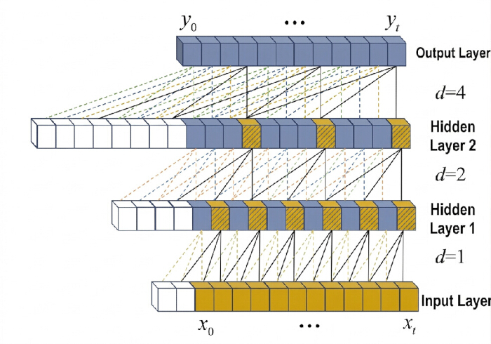
Figure 1: Dilated Causal Convolution Structure. Schematic illustration of the temporal convolutional network (TCN) architecture employing causal and dilated convolutions. The dilation factor increases with network depth to expand the receptive field and capture long-range temporal dependencies in acoustic signals. Please click here to view a larger version of this figure.

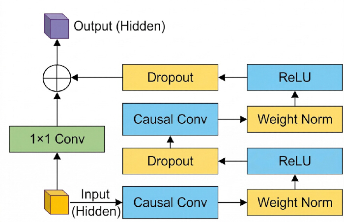
Figure 2: Residual Connection Structure. Diagram of the residual block used within the TCN architecture. The block incorporates causal convolutions, weight normalization, ReLU activation functions, dropout layers, and a residual connection to facilitate stable deep-network training and mitigate gradient degradation. Please click here to view a larger version of this figure.

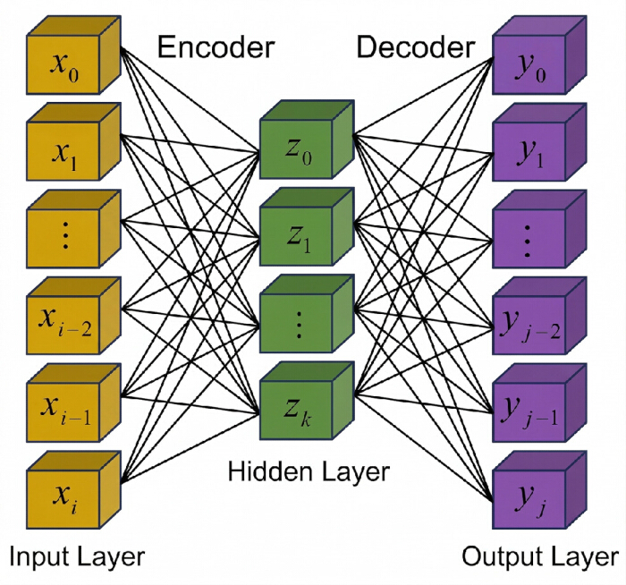
Figure 3: Autoencoder (AE) Architecture. Schematic representation of the AE used for feature-dimension reduction. The encoder compresses the input acoustic features into a latent representation, and the decoder reconstructs the original feature space from the compressed representation. Please click here to view a larger version of this figure.

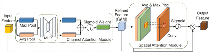
Figure 4: Convolutional Block Attention Module (CBAM) Architecture. Workflow of the CBAM used for frequency-domain feature enhancement. The module sequentially applies channel-attention and spatial-attention mechanisms to refine feature representations extracted from Mel spectrograms. Please click here to view a larger version of this figure.

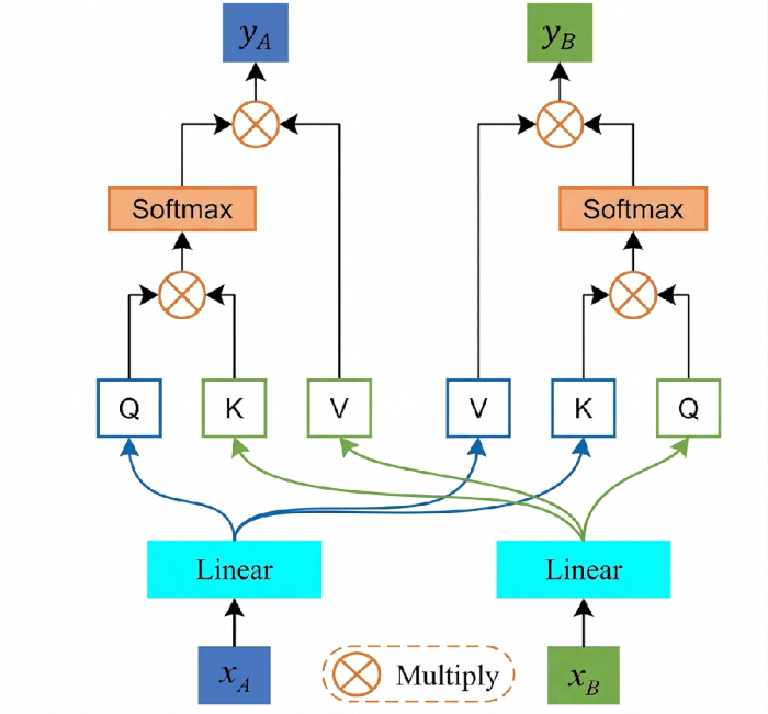
Figure 5: Cross-Attention (CA) Feature Fusion Mechanism. Schematic representation of the CA module used to fuse temporal and frequency-domain features. Query, Key, and Value matrices are generated from the two feature modalities to model cross-modal dependencies and produce fused feature representations. Please click here to view a larger version of this figure.

1. Setup of the Insulation Fault Acoustic Fingerprint Platform and Data Acquisition

1. Construct a non-contact microphone array detection platform within the laboratory. Assemble the system using a high-voltage test circuit, a test cabinet containing defect models, a Transient Earth Voltage (TEV) testing system, and the microphone array system. The TEV system was operated as the electrical reference channel for discharge verification.
   NOTE: Ensure that the high-voltage circuit includes an autotransformer (T1), a test transformer (T2), a 200 kΩ protective resistor (R), and a 1 nF coupling capacitor (Cx). Refer to Figure 6 for the schematic layout.
   CAUTION: High-voltage testing presents a risk of electrical shock. Follow institutional electrical safety procedures and ensure that all high-voltage components are properly insulated and grounded before operation.
2. Configure four distinct insulation fault models inside the test cabinet to simulate common operational defects: surface discharge, suspended discharge, internal discharge, and point discharge (Figure 7).
3. Prepare the insulation fault models for testing.
   1. Fabricate all models on 100 mm × 100 mm × 5 mm epoxy-resin insulating plates using polished electrodes.
   2. Prepare the surface-discharge model by fixing two 20 mm × 10 mm × 1 mm copper strip electrodes on the upper surface with a 15 mm creepage gap. Leave the intervening epoxy surface exposed.
   3. Prepare the suspended-discharge model by mounting a 2 mm-diameter copper rod electrode 5 mm above a grounded copper plate (40 mm × 40 mm × 1 mm) using an epoxy support. Keep the rod electrode electrically isolated from the plate.
   4. Prepare the internal-discharge model by casting an epoxy block containing a cylindrical artificial air void (10 mm diameter × 2 mm height) centered between two copper plates (40 mm × 40 mm × 1 mm). Position the void center approximately 2.5 mm below the upper surface.
   5. Prepare the point-discharge model by positioning a stainless-steel needle electrode with an approximate 0.5 mm tip radius opposite a grounded copper plate across a 10 mm air gap.
   6. Clean all electrodes with ethanol and dry them completely before assembly.
   7. Assemble the electrode-defect geometry in the test cabinet and verify all electrode spacings using a caliper before each voltage test.
4. Deploy the microphone array sensor employing a modified annular spiral structure consisting of 112 channels. Refer to Figure 8 for the coordinate distribution.
5. Set the sampling rate to 200 kHz and configure the sample length to 8192 points per frame. Refer to Table 1 for the sensor parameters.
6. Configure the microphone array hardware.
   1. Mount the 112 microphones flush on the modified annular spiral frame at the coordinate positions shown in Figure 8. Maintain the inter-element spacing defined by the array-coordinate file, ranging from 10 mm to 25 mm.
   2. Position a portable acoustic calibrator and a 40 kHz ultrasonic reference source 300 mm from the center of the microphone array.
   3. Calibrate all active microphone channels before each acquisition session using a 94 dB SPL, 1 kHz acoustic reference signal and a 40 kHz ultrasonic reference signal.
   4. Record 5 s calibration signals from each microphone channel.
   5. Calculate the RMS sensitivity and phase response of each channel relative to the array-center channel.
   6. Retain only channels with a sensitivity deviation within ±2 dB at 1 kHz, within ±3 dB at 40 kHz, and without clipping or abnormal noise-floor elevation.
   7. Exclude channels that do not satisfy the acceptance criteria from subsequent analysis.
   8. Repeat the calibration procedure after any microphone replacement or movement of the microphone array.
7. Configure the multichannel data-acquisition system to perform simultaneous sampling across all active microphone channels.
   1. Configure the DAQ system for simultaneous acquisition of all 112 microphone channels using a shared 200 kHz sampling clock.
   2. Set the acquisition resolution to 16 bits, configure AC coupling, and acquire 8192 points per frame.
   3. Distribute a hardware start trigger to all acquisition modules through a common positive-edge TTL trigger bus.
   4. Store all microphone channels within the same frame record and retain the trigger timestamp and channel index for each acquisition.
   5. Inspect the first 100 acquired frames for dropped samples, channel saturation, and clock drift before beginning formal data collection.
8. Justify the microphone array configuration. The 112-channel array was selected to improve spatial sampling density for beamforming and GCC-PHAT delay estimation, thereby increasing suppression of off-axis environmental noise relative to a sparse low-channel-count array. Although approximately four channels can be sufficient for geometric 3D localization, the present protocol uses dense spatial sampling for signal enhancement and feature stability rather than localization alone. Reduced-channel versions should be validated separately before cost-sensitive field deployment.
9. Apply high voltage to the test circuit to induce partial discharge phenomena across the models.
10. Maintain the experimental environment during testing.
    1. Maintain the laboratory at 22°C ± 2°C, 45%–55% relative humidity, and 101 ± 2 kPa atmospheric pressure during data acquisition.
    2. Measure the background acoustic noise before energizing the high-voltage system.
    3. Proceed with data acquisition only when the A-weighted background noise level is ≤40 dB(A).
    4. Verify that the ultrasonic noise floor of each active microphone channel is at least 20 dB below the discharge-impulse level observed during pilot testing.
    5. Keep doors and windows closed and switch off nonessential rotating equipment during data collection.
    6. Ground the high-voltage frame and DAQ chassis before acquisition.
    7. Prevent personnel movement near the microphone array during recording.
11. Monitor the discharge activity continuously utilizing the TEV sensor connected to a PC terminal.
    1. Set the TEV monitoring threshold to 6 dB above the pre-test background noise floor and not lower than an equivalent input level of 10 mV.
    2. Configure the TEV reference channel with an analog bandwidth of 3–100 MHz and a gain of 40 dB.
    3. Record TEV pulse activity using envelope and pulse logging on the PC terminal.
    4. Configure the TEV system to use positive-edge hardware triggering.
    5. Use the same threshold value for both TEV monitoring and trigger generation.
    6. Accept an acoustic frame only when TEV pulse activity occurs within the corresponding acquisition window and is repeated across consecutive frames at the selected voltage.
12. Adjust the voltage progressively between 4 and 12 kV.
13. Record the acoustic signals once a distinct and stable insulation fault phenomenon is observed for a specific model. Define a distinct and stable fault phenomenon as a discharge state in which TEV activity and acoustic impulse patterns are repeatedly observed at the target voltage without obvious intermittent extinction, acoustic-channel saturation, unrelated mechanical noise, or external impact noise. Maintain the voltage until the discharge pattern remains stable for at least 60 s before recording acoustic frames.
14. Collect 1000 sets of valid data for each of the four fault types. Classify a sample frame as valid only when the TEV reference indicates discharge activity, the acoustic channel is not saturated, the frame contains no obvious external impact or handling noise, and the sample label matches the active defect model. Exclude frames with acoustic-channel saturation, absent TEV confirmation, inconsistent fault labeling, intermittent discharge extinction, external mechanical impact, or unstable background noise.
15. Synchronize the TEV system and acoustic acquisition system during data collection.
    1. Connect the TEV trigger output to the acoustic DAQ trigger input through the shared TTL trigger bus.
    2. Use the TEV pulse output as the hardware trigger for acoustic data acquisition.
    3. Record the trigger marker as a digital timing channel in the acoustic data file.
    4. Perform initial alignment of the TEV and acoustic acquisition streams using the trigger timestamp.
    5. Estimate residual inter-microphone delays using GCC-PHAT before beamforming.
    6. Verify that the TEV-acoustic synchronization accuracy is within ±1 acoustic sample, corresponding to ≤5 μs at a sampling rate of 200 kHz.

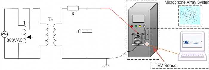
Figure 6: Insulation Fault Detection Platform with Microphone Array. Experimental setup used for acoustic insulation-fault detection. The platform consists of a high-voltage test circuit, insulation-fault test cabinet, microphone array system, TEV sensor, and computer-based monitoring system for data acquisition and verification. Please click here to view a larger version of this figure.

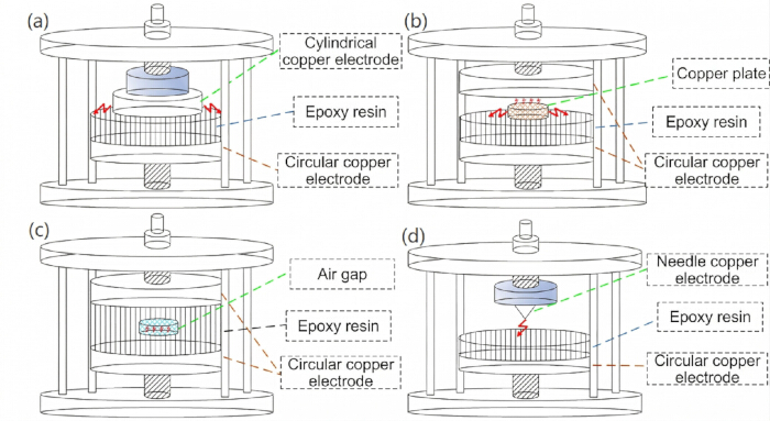
Figure 7: Laboratory-Constructed Insulation Fault Models. Representative insulation-fault models used for data acquisition. (A) Surface discharge model. (B) Suspended discharge model. (C) Internal discharge model. (D) Point discharge model. The models were constructed to simulate four common insulation-fault conditions under controlled laboratory conditions. Please click here to view a larger version of this figure.

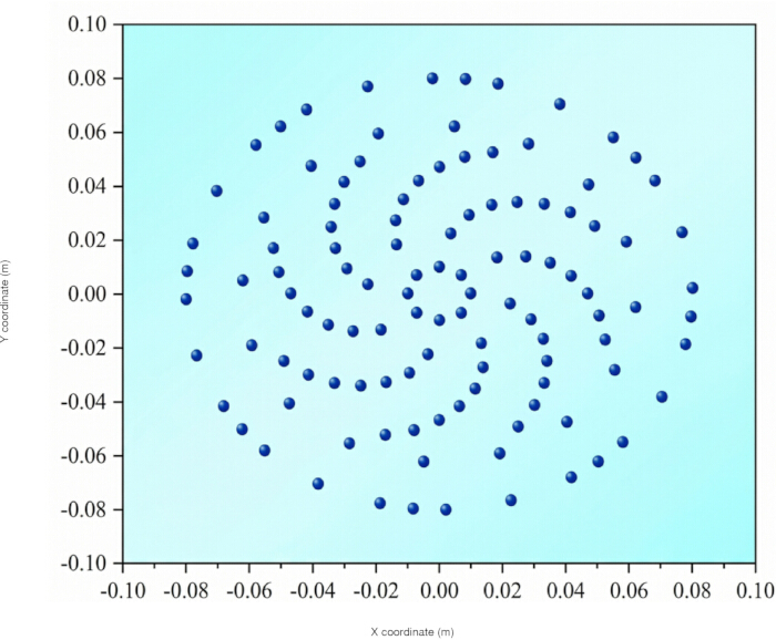
Figure 8: Microphone Array Distribution. Spatial arrangement of the 112-channel microphone array employing a modified annular spiral configuration. The coordinate distribution illustrates the sensor placement used for acoustic signal acquisition and subsequent beamforming analysis. Please click here to view a larger version of this figure.

Parameter Type	Parameter Value
Array structure	Modified annular spiral
Number of channels	112
Sampling rate	200 kHz
Sample points per frame	8192

Table 1: Microphone Array Parameters. Technical specifications of the microphone array system used for acoustic signal acquisition during insulation-fault experiments. The table summarizes the array geometry, number of channels, sampling rate, and the number of sample points acquired per frame. Please click here to download this Table.

2. Time-Domain Feature Extraction via TCN-AE

1. Input the pre-processed time-series acoustic data into the TCN to capture dynamic temporal variations^13,14. After signal fusion, normalize each 8192-point acoustic frame using the normalization procedure applied during model training and input the normalized 1D sequence into the TCN.
2. Configure the TCN architecture.
   1. Construct the TCN using three residual blocks arranged sequentially for temporal feature extraction.
   2. Assign 64 convolutional filters to each residual block and set the convolution kernel size to 3.
   3. Implement dilated causal convolutions and configure the dilation factors as d = 1, 2, and 4 to progressively expand the temporal receptive field.
   4. Apply the ReLU activation function after each convolutional operation.
   5. Apply a dropout rate of 0.20 after each residual block to reduce overfitting during training.
   6. Perform weight normalization as the regularization method within each residual block.
   7. Incorporate residual connections throughout the network and use 1 × 1 convolutional projections whenever necessary to match feature dimensions between the residual and transformed pathways.
3. Apply causal convolutions to the input sequence. Adapt the zero-padding prior to the sequence based on the kernel size to ensure that the output at any given time step depends strictly on current and previous inputs.
4. Execute the causal convolution using the kernel weight (w_i) and kernel size (K) as follows (Equation 1):
      (1)
5. Implement dilated convolutions to expand the receptive field of the network without increasing the parameter count. Increase the dilation factor d exponentially as the network depth advances to capture long-range temporal dependencies.
6. Calculate the dilated convolution using the dilation factor (d) as follows (Equation 2). Use the dilation-factor progression d = 1, 2, and 4 during TCN training to progressively expand the temporal receptive field without increasing the number of sampled points in each acoustic frame.
      (2)
7. Integrate residual connections to mitigate vanishing gradients during deep network training.
8. Pass the input sequence through the dilated causal convolution block. Perform weight regularization and apply a ReLU non-linear activation followed by a Dropout layer.
9. Add the processed output directly to the original input sequence (Figure 2). Apply weight normalization within each residual block and use a dropout rate of 0.20 before performing the residual addition. Use a 1 × 1 convolutional projection when necessary to match feature dimensions between the residual and transformed pathways.
10. Feed the high-dimensional temporal features extracted by the TCN into an AE for feature-dimension reduction¹⁵.
11. Configure the AE architecture.
    1. Construct the encoder using three fully connected layers with dimensions 512, 256, and 128 neurons, respectively.
    2. Define the latent-space representation using a 128-dimensional feature vector.
    3. Construct the decoder using three fully connected layers with dimensions 128, 256, and 512 neurons, respectively.
    4. Apply the ReLU activation function after each fully connected layer in both the encoder and decoder.
    5. Configure the AE to reconstruct the input feature representation from the latent-space vector and optimize the reconstruction using the mean squared error (MSE) loss function described in Step 2.16.
12. Compress the input data into a lower-dimensional latent-space representation via the encoder.
13. Reconstruct the original data using the decoder (Figure 3).
14. Execute the encoding and decoding transformations using the ReLU activation function (σ), weight matrices (W₁ and W₂), and bias terms (b₁ and b₂) as given by Equations 3 and 4.
       (3)
      (4)
15. Train the AE to preserve critical information by minimizing the reconstruction error.
16. Utilize the mean squared error (MSE) as the loss function and calculate the reconstruction error using Equation 5.
    1. Train the AE using the Adam optimizer with a learning rate of 0.001.
    2. Set the batch size to 50 and train the network for a maximum of 100 epochs.
    3. Monitor the validation loss during training and apply early stopping with a patience value of 10 epochs.
    4. Use the fixed dataset partition consisting of 2400 training samples, 400 validation samples, and 400 testing samples.
    5. Perform model training in the Python-based deep-learning environment summarized in the Table of Materials.
    6. Calculate the reconstruction error using Equation 5.
         (5)

3. Frequency-Domain Feature Extraction via Mel Spectrogram and CBAM

1. Apply pre-emphasis, framing, and windowing functions to the raw partial-discharge acoustic signals.
   1. Remove the DC offset from each 8192-point acoustic frame.
   2. Apply pre-emphasis using:
      
   3. Normalize each frame using its peak absolute amplitude after DC-offset removal.
   4. Segment each frame using a 1024-sample Hamming window.
   5. Use a hop length of 512 samples, corresponding to 50% overlap between adjacent windows.
   6. Compute the short-time Fourier transform (STFT) using a 1024-point FFT.
   7. Do not apply additional software band-pass filtering beyond the hardware front-end bandwidth limitation and the frame-quality exclusion criteria described above.
2. Perform a Fourier transform on the processed signals.
3. Convert the original linear frequency (f) to the Mel scale. This step linearizes human frequency perception and reduces the weight of interference bands¹⁶.
4. Calculate the Mel-scale frequency (f_mel) using the original linear frequency (f) (Equation 6).
      (6)
5. Partition the frequencies into a sequence of triangular filter banks.
6. Calculate the weighted sum of all signal amplitudes within each filter bandwidth. Apply a logarithmic function to the output to enhance perceptual consistency regarding amplitude variations.
7. Calculate the Mel-filter-bank output using Equation 7. Here, S(m) is the output of the m-th filter, k is the frequency index, and H_m(k) defines the triangular filter.
     (7)
8. Generate the Mel spectrograms.
   1. Compute the short-time Fourier transform using an FFT size of 1024.
   2. Apply 256 Mel filter banks to the resulting frequency spectrum.
   3. Generate Mel-spectrograms over the frequency range of 0–100 kHz.
   4. Resize or represent the resulting Mel spectrograms as 256 × 256-pixel feature maps for subsequent CBAM processing.
   5. Convert the Mel power spectrogram to the decibel scale.
   6. Apply per-spectrogram min-max normalization using the logarithmically compressed Mel spectrogram (S_dB):
      
   7. Perform the normalization independently for each 256 × 256 Mel-spectrogram image.
   8. Clip the normalized values to the range [0,1] before inputting the spectrogram into the CBAM branch.
9. Input the resulting Mel spectrograms into the CBAM to extract principal spectral characteristics¹⁷.
10. Process the data through sequential channel-attention and spatial-attention mechanisms (Figure 4).
11. Configure the CBAM architecture.
    1. Configure the channel-attention module using a channel-reduction ratio of 16.
    2. Process input feature maps with dimensions of 256 × 256 × 64.
    3. Apply global average pooling and global max pooling to generate channel descriptors.
    4. Pass the pooled descriptors through a shared multilayer perceptron and apply a Sigmoid activation function to generate channel-attention weights.
    5. Generate spatial-attention weights using a 3 × 3 convolutional kernel applied to the concatenated average-pooled and max-pooled spatial descriptors.
    6. Apply a Sigmoid activation function to produce the final spatial-attention map.
12. Extract the channel-attention weights.
13. Apply global average pooling  and global max pooling  across the channel dimensions of the input feature map.
14. Process the generated global descriptor vectors through a fully connected (FC) layer to obtain the channel-attention weight (M_c).
15. Calculate the channel-attention weights using Equation 8. Here, M_c is the channel-attention weight, FC denotes the fully connected layer, and σ represents the Sigmoid activation function.
      (8)
16. Extract the spatial-attention weights.
17. Apply global max pooling  and global average pooling  along the channel axis.
18. Concatenate the resulting spatial descriptor maps and process them through a convolutional layer to generate the spatial-attention weight (M_s).
19. Calculate the spatial-attention weights using Equation 9. Here, M_s is the spatial-attention weight,  is the spatial descriptor generated by global average pooling, and  is the spatial descriptor generated by global max pooling.
       (9)
    1. Concatenate the average-pooled and max-pooled spatial descriptors along the channel dimension.
    2. Apply a 3 × 3 convolution  with stride = 1 and same padding to generate the spatial-attention feature map.
    3. Apply a Sigmoid activation function to the convolution output to obtain the spatial-attention weights.
    4. Multiply the spatial-attention weights element-wise with the input feature map to generate the refined spatial representation.

4. Cross-Modal Feature Fusion Using CA

1. Implement a CA mechanism to synthesize the extracted temporal features and spectral features¹⁸. Unlike self-attention, extract contextual information from one modality to dynamically enhance the representation of the other (Figure 5).
2. Configure the CA architecture.
   1. Set the embedding dimension to 128.
   2. Configure the CA module with 4 attention heads.
   3. Set the Query, Key, and Value projection dimensions to 128 each.
   4. Apply a dropout rate of 0.10 within the CA module.
   5. Do not apply post-attention normalization layers or feed-forward layers after the cross-attention module.
   6. Concatenate the outputs from all attention heads.
   7. Apply dropout with a rate of 0.10.
   8. Flatten the resulting feature representation.
   9. Transfer the flattened feature vector directly to the 1D-CNN classifier.
3. Initialize the Query (Q), Key (K), and Value (V) matrices from the two distinct input sequences (time- and frequency-domain features).
4. Calculate the Query matrix using Equation 10, where X₁ denotes the temporal feature matrix produced by the TCN-AE pathway, and W_Q, and b_Q indicates the corresponding learned weight matrix and bias term, respectively.
      (10)
5. Calculate the Key matrix using Equation 11, where X₂ denotes the frequency-domain feature matrix produced by the Mel-CBAM pathway, and W_K, and b_K indicates the corresponding learned weight matrix and bias term, respectively.
      (11)
6. Calculate the Value matrix using Equation 12. where W_V and b_V indicates the corresponding learned weight matrix and bias term, respectively.
      (12)
7. Compute the CA interaction based on the relationship between the Query and Key elements.
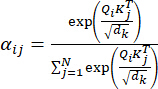
8. Calculate the attention-weight matrix using Equation 13. Here, α_ij specifies the attention weight of the i-th element relative to the j-th element, and d_k is the dimensionality of the key vectors.
      (13)
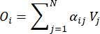
9. Update the final feature representation by computing the weighted sum of the Value matrix according to the calculated attention weights.
10. Calculate the fused feature representation using Equation 14. Here, O_i is the sequence output representing the robust fused time-frequency acoustic fingerprint of the insulation fault.
    ​   (14)
    1. Generate the fused feature representation with an output dimension of 128.
    2. Combine the cross-time and cross-frequency attention outputs.
    3. Flatten the fused representation before classification.
    4. Pass the flattened feature representation to the 1D-CNN and fully connected Softmax classifier shown in Figure 9.

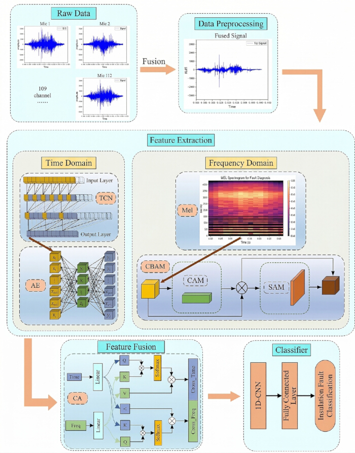
Figure 9: Overall Framework for Insulation Fault Identification. Workflow of the proposed insulation-fault identification method. Raw microphone-array signals are fused and preprocessed, followed by time-domain feature extraction using a TCN–AE pathway, frequency-domain feature extraction using Mel spectrograms and CBAM, CA-based feature fusion, and final fault classification using a one-dimensional convolutional neural network. Please click here to view a larger version of this figure.

5. Align and Fuse Microphone Array Signals via GCC-PHAT

1. Select two microphone signals for delay estimation and convert them to the frequency domain using the FFT.
   1. Use the full 8192-point acoustic frame acquired at 200 kHz for the FFT-based GCC-PHAT calculation.
   2. Apply the FFT to each selected microphone signal before computing the PHAT-weighted cross-power spectrum.
   3. Estimate the inter-channel time delay relative to the selected reference microphone using the PHAT-weighted cross-power spectrum and IFFT procedure shown in Figure 10.
   4. Apply GCC-PHAT relative to the selected reference microphone before aligning all 112 active microphone channels.
   5. Apply a Hann window to the full 8192-point acoustic frame before FFT processing.
   6. Do not use overlapping windows during GCC-PHAT delay estimation.
   7. Zero-pad each windowed frame to 16,384 points before FFT and IFFT computation.
   8. Use the zero-padded signal to improve delay-peak resolution during time-delay estimation.
2. Obtain the frequency-domain representations  and  of the selected microphone signals.
3. Calculate the cross-power spectrum to evaluate the similarity between the two signals.
4. Introduce the phase transform (PHAT) weighting function to sharpen the cross-correlation peak and mitigate reverberation effects.
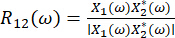
5. Calculate the PHAT-weighted cross-power spectrum using Equation 15. Here,  and  are the frequency-domain representations of the two microphone signals and  denotes the complex conjugate.
      (15)
6. Apply the IFFT to compute the generalized cross-correlation (GCC) function.
7. Identify the time-delay variable τ by locating the peak of the GCC function.
8. Calculate the GCC function using Equation 16. Here,  is the generalized cross-correlation function and represents the estimated time delay.
      (16)
9. Perform time compensation to align the signals based on the estimated delay.
10. Synchronize each channel  relative to the reference microphone using Equation 17. Here,  is the delay-compensated signal and τ_i is the estimated delay relative to the reference microphone.
    1. Select the microphone located closest to the geometric center of the array as the reference microphone.
    2. Verify that the selected microphone satisfies the calibration acceptance criteria described in Step 1.6.
    3. If the center microphone does not satisfy the calibration criteria, select the nearest calibrated microphone to the geometric center as the reference microphone.
    4. Estimate the delay τ_i for each active microphone channel relative to the selected reference microphone.
    5. Align all 112 active microphone channels to the selected reference microphone before beamforming.
          (17)
11. Execute delay-and-sum beamforming to fuse the spatial information.
12. Enhance the signal originating from the target direction while suppressing ambient noise using Equation 18. Here, y(t) is the beamformed output signal,  is the delay-compensated signal from the i-th microphone, and N is the total number of microphone channels.
    1. Perform delay-and-sum beamforming after GCC-PHAT delay compensation.
    2. Use equal weighting for all active microphone channels.
    3. Set N = 112 for the 112 active microphone channels used during acquisition.
    4. Define the target direction using the known geometric location of the active defect model relative to the microphone-array center.
    5. Steer the delay-and-sum beamformer toward the center of the active defect model during signal fusion.
    6. Use the predefined test-cabinet geometry to determine the steering direction.
    7. Do not perform data-driven target-direction estimation during model training or testing.
          (18)

Figure 10: GCC-PHAT Signal Alignment Procedure. Workflow of the generalized cross-correlation with phase transform (GCC-PHAT) algorithm. Frequency-domain microphone signals are processed to obtain the cross-power spectrum and weighting function, followed by inverse Fourier transformation to estimate inter-channel time delay. Please click here to view a larger version of this figure.

6. Optimize the Network via the CS Algorithm

1. Initialize the CS algorithm parameters to optimize the 1D-CNN.
   1. Set the population size, corresponding to the number of nests, to 20.
   2. Set the discovery probability (Pa) to 0.25.
   3. Set the maximum number of optimization iterations to 50.
   4. Set the random seed to 42 to support reproducibility.
   5. Set the step-size scaling parameter α to 0.01.
   6. Define the hyperparameter search bounds according to the ranges summarized in Table 2.
   7. Terminate optimization when the maximum number of iterations is reached or when validation-fitness convergence is achieved.
2. Generate new solutions by simulating the obligate brood parasitism behavior of cuckoos combined with Lévy flights.
3. Update the current solution (nest)  using a random step size derived from the Lévy flight characteristic.
4. Calculate the updated nest position using Equation 19. Here, α is the step-size scaling parameter and  denotes entry-wise multiplication.
   1. Set the step-size scaling parameter (α) to 0.01.
   2. Set the Lévy-flight parameter (λ) to 1.5.
   3. Encode each candidate nest as a set of 1D-CNN hyperparameters, including convolutional-layer configuration, kernel size, learning rate, batch size, and optimizer setting.
   4. Generate candidate nests using Lévy-flight updates and evaluate each candidate using validation-set performance.
   5. Retain candidate solutions that improve validation fitness.
         (19)
5. Calculate the random variables for the Lévy flight using a standard normal distribution scaled by the parameter σ.
6. Calculate σ using Equation 20. Here,  represents the Gamma function and β is typically set to 1.5.
      (20)
7. Train the 1D-CNN using five convolutional layers, a kernel size of 3, ReLU activation, stochastic gradient descent (SGD) optimization, an initial learning rate of 0.001, a batch size of 50, and a cross-entropy loss function.
8. Evaluate the optimized model on the testing set.
   1. Train the final 1D-CNN using validation-loss early stopping with a patience value of 10 epochs.
   2. Set the random seed to 42 for dataset partitioning and model training.
   3. Evaluate the optimized model using the fixed testing set summarized in Table 2.
   4. Report the full confusion-matrix evaluation separately from the ablation result, with an overall accuracy of 99.05% (3962/4000) and class-wise recognition rates ranging from 98.6% to 99.4%.

Category	Parameter	Value / Setting
Dataset and input	Total acoustic frames	4,000
	Fault classes	Surface discharge; suspended discharge; internal discharge; point discharge
	Sampling rate	200 kHz
	Frame length	8,192 points per frame
	Microphone-array channels	112
	Model input	Cross-attention fused time-frequency acoustic feature representation
Dataset split	Training set size	2,400 samples
	Validation set size	400 samples
	Testing set size	400 samples
	Full confusion-matrix evaluation size	4,000 samples
	Split strategy	Single fixed split
	Random seed	42
TCN architecture	Number of residual blocks	3
	Filters per residual block	64
	Convolution kernel size	3
	Dilation schedule	1, 2, 4
	Dropout rate	0.20
Autoencoder architecture	Encoder-layer dimensions	512 → 256 → 128
	Latent-space dimension	128
	Decoder-layer dimensions	128 → 256 → 512
Autoencoder training	Optimizer	Adam
	Learning rate	0.001
	Batch size	50
	Number of training epochs	100 epochs
	Early stopping criterion	Validation MSE; patience = 20 epochs
Mel-spectrogram settings	FFT size	1,024 points
	Number of Mel filters	256
	Frequency range	0–100 kHz
	Spectrogram dimensions	256 × 256
CBAM configuration	Channel-reduction ratio	16
	Feature-map dimensions	256 × 256 × 64
Cross-attention configuration	Embedding dimension	128
	Number of attention heads	4
	Query projection dimension	128 total; 32 per head
	Key projection dimension	128 total; 32 per head
	Value projection dimension	128 total; 32 per head
	Dropout rate	0.10
1D-CNN classifier	Number of convolutional layers	5
	Convolution kernel size	3
	Activation function	ReLU
	Output layer	4-class Softmax
	Loss function	Cross-entropy loss
Training settings	Optimizer	Stochastic Gradient Descent (SGD)
	Initial learning rate	0.001
	Batch size	50
	Maximum training iterations	1,000
	Early stopping	Validation-loss monitoring
	Early-stopping patience	100 iterations
	Final training loss	Not available in supplied manuscript
	Final validation loss	Not available in supplied manuscript
Cuckoo Search optimization	Optimization target	1D-CNN hyperparameters
	Population size / number of nests	20
	Discovery probability (Pa)	0.25
	Step-size scaling parameter (α)	0.01
	Lévy-flight parameter (β)	1.5
	Lévy-flight parameter (λ)	1.5
	Maximum optimization iterations	50
	Hyperparameter search bounds	Conv filters {32, 64, 128, 256}; kernel size {3, 5, 7}; learning rate 1×10⁻⁴–1×10⁻²; batch size {25, 50, 100}; dropout 0.10–0.50; weight decay 1×10⁻⁵–1×10⁻³
Validation and reporting	Figure 13 CA ablation accuracy	98.20%
	Table 2 confusion-matrix accuracy	99.05% (3,962/4,000)
	Cross-validation / repeated runs	Not performed

Table 2: Dataset configuration, model-training parameters, and optimization settings for insulation-fault classification. The table summarizes the dataset composition, data partitioning strategy, 1D-CNN architecture, training configuration, Cuckoo Search optimization settings, validation metrics, and parameter-selection considerations used to develop and evaluate the proposed fault-diagnosis framework. Missing implementation-specific values should be reported from the final training and optimization logs to facilitate reproducibility. Please click here to download this Table.

Results

Time- and Frequency-Domain Feature Extraction Framework

The proposed insulation-fault identification method integrates temporal and spectral feature extraction pathways to characterize the complex acoustic signatures generated by insulation defects. Time-domain feature extraction was performed using a TCN incorporating dilated causal convolutions to capture long-range temporal dependencies within the acoustic sequences (Figure 1). Residual connect...

Discussion

This method article delineates a standardized, non-contact protocol for identifying complex insulation faults in electrical power equipment through acoustic fingerprint recognition. By integrating a TCN-AE alongside a Mel spectrogram processed by a Mel-CBAM, the established pipeline isolates both dynamic time-series fluctuations and localized spectral characteristics. The subsequent cross-modal fusion via a CA mechanism is intended to reduce the information dilution that often accompanies simple feature concatenation. Op...

Materials

List of materials used in this article

Name	Company	Catalog Number	Comments
Autoencoder (AE)	Custom model	Encoder-decoder architecture for feature compression	Feature dimensionality reduction
Cross-Attention module	Custom model	Time-frequency feature fusion module	Cross-modal feature fusion
GCC-PHAT algorithm	Custom algorithm	FFT/IFFT-based implementation	Time-delay estimation and signal alignment
High-voltage test circuit	Self-built laboratory platform	Autotransformer T1, test transformer T2, 200 kΩ protective resistor, 1 nF coupling capacitor; operating voltage 4–12 kV	Generation of insulation-fault conditions
Mel spectrogram + CBAM	Custom model	Mel-frequency spectral extraction with attention enhancement	Frequency-domain feature extraction
Microphone array system	Self-built laboratory platform	112-channel modified annular spiral array; 200 kHz sampling rate; 8192 points per frame	Acoustic acquisition
Microphone sensors	Self-built matched ultrasonic microphone modules	112 matched channels; sensitivity -38 +/- 3 dBV/Pa; 20 Hz-100 kHz frequency response; calibrated at 94 dB SPL/1 kHz and 40 kHz; acceptance limits: +/-2 dB at 1 kHz and +/-3 dB at 40 kHz	Acoustic detection
Multichannel DAQ system	Self-built synchronized DAQ platform	112-channel simultaneous acquisition; 16-bit ADC; 200 kHz/channel; 8192 points/frame; shared sampling clock; positive-edge TTL hardware trigger	Data acquisition and synchronization
One-dimensional CNN + CS optimization	Custom model	Five convolutional layers; kernel size 3; SGD; learning rate 0.001; batch size 50	Fault classification
Python training environment	Python / PyTorch	Python 3.9; PyTorch 2.0; NumPy 1.24; scikit-learn 1.2; librosa 0.10; CUDA 11.8	Model training and evaluation
Temporal Convolutional Network (TCN)	Custom model	Dilated causal convolutions with residual connections	Time-domain feature extraction
Test cabinet with defect models	Self-built laboratory platform	Surface discharge, suspended discharge, internal discharge, and point discharge models	Simulation of insulation faults
Transient Earth Voltage (TEV) testing system	Commercial TEV monitoring module	TEV reference channel; 3-100 MHz analog bandwidth; 40 dB gain; positive-edge TTL trigger; trigger threshold set 6 dB above background noise floor or >=10 mV equivalent at sensor input	Verification of discharge activity