This study of 21 OECD countries (2000-2020) finds that the Environmental Policy Index, greenhouse gas emissions, and environment-related technology facilitate renewable energy adoption, while Green GDP hinders it. A two-way causal relationship exists among all variables. The pace of transition remains insufficient, requiring policy reforms and pollution taxes.
A subscription to JoVE is required to view this content. Sign in or start your free trial.
Research Article
The Influence of Environmental Policies and Technologies on the Transition to Renewable Energy
In This Article
Summary
Abstract
Renewable energy capacity (REC) plays a central role in achieving sustainable development and carbon neutrality, yet the effects of ecological policy performance, environmental quality, technological innovation, and green economic growth on REC remain heterogeneous across countries and stages of renewable energy development. This study investigates the determinants of renewable energy capacity across 21 OECD countries from 2000 to 2020, focusing on ecological policy performance (EPI), greenhouse gas (GHG) emissions, eco-friendly technology (EFT), and Green GDP. The empirical framework employs the Panel Autoregressive Distributed Lag (ARDL) bounds testing approach to examine long-run cointegration, the Method of Moments Quantile Regression (MMQR) to capture heterogeneous effects across the conditional distribution of REC, and panel Granger causality tests to determine the direction of causal relationships. The Panel ARDL bounds test confirms a stable long-run equilibrium relationship among the variables (F = 7.845, p < 0.01). MMQR results show that EPI exerts a positive and progressively stronger effect across quantiles (0.092–0.212), while EFT exhibits the steepest positive gradient (0.131–0.221) and demonstrates bidirectional causality with REC, indicating a reinforcing cycle between technological innovation and renewable energy deployment. GHG emissions have a modest positive association with REC (0.048–0.082) but do not unidirectionally cause REC; instead, higher renewable energy capacity significantly reduces emissions. Green GDP consistently exhibits a negative effect on REC (−0.348 to −0.138), although this effect weakens at higher renewable energy capacity quantiles, suggesting a transitional adjustment during the shift toward a greener economy. These findings indicate that the effects of environmental policy, technological innovation, emissions, and green economic performance are stage-dependent, highlighting the need for deployment-specific policy frameworks, sustained investment in green research and development, and complementary policy instruments to mitigate short-term adjustment costs while accelerating the renewable energy transition.
Introduction
Escalating global energy demand has intensified the need for a rapid transition to clean energy sources. Although renewable energy accounted for approximately 30% in solar energy supply growth, fossil fuels continue to dominate incremental energy demand, resulting in the continued accumulation of carbon dioxide (CO2) emissions and threatening the achievement of the Paris Agreement targets1. A systematic understanding of sustainable energy investment trends, as illustrated through the scientific mapping and meta-analysis presented in Financing the Future: Insights into Sustainable Energy Investments, highlights the convergence of policy, financial, and technological transformations that occurred across OECD economies between 2000 and 20202. This twenty-year period, encompassing 21 OECD countries, provides an ideal setting for evaluating the long-run determinants of renewable energy deployment3. The renewable energy transition depends on the effective interaction of environmental governance, financial investment, and technological innovation4. A recent systematic review identified economic and policy factors as the principal drivers of renewable energy expansion. Threshold analyses of OECD countries further demonstrated that environmental policy stringency promotes renewable energy deployment only after surpassing a critical threshold5, while the diffusion of eco-friendly technologies similarly requires sustained investment before significant benefits are realized6. Moreover, dynamic panel quantile regression analyses across 77 countries have shown that eco-friendly technologies significantly promote renewable energy consumption, particularly in developing economies7.
Despite these advances, several important research gaps remain. Existing studies typically examine environmental policy and technological innovation in isolation, overlooking their potential synergies in renewable energy deployment. In addition, renewable energy capacity (REC), used in this study as the dependent variable, has received limited attention within integrated empirical frameworks that simultaneously consider environmental policy, technological innovation, emissions, and green economic performance8. Furthermore, momentum toward renewable energy adoption in advanced economies has slowed. OECD greenhouse gas (GHG) emissions remain high, while climate policy stringency increased by only 1% in 2024, highlighting an implementation gap that warrants deeper investigation into renewable energy drivers in high-income economies9. Accordingly, this study examines the determinants of renewable energy capacity across 21 OECD countries from 2000 to 2020 using the Ecological Performance Index (EPI), greenhouse gas (GHG) emissions, eco-friendly technology (EFT), and Green GDP as explanatory variables. Following preliminary diagnostic testing, the Panel ARDL bounds cointegration test is employed to establish long-run equilibrium relationships, the Method of Moments Quantile Regression (MMQR) is applied to capture distributional heterogeneity, and panel causality tests are conducted to determine the direction of causal relationships10. The findings demonstrate that EPI and EFT exert significant positive effects only beyond specific thresholds, whereas the influence of Green GDP varies across the conditional distribution of renewable energy capacity, emphasizing the importance of coordinated environmental policy, technological innovation, and economic strategies11. By explicitly modeling the joint effects of environmental policy performance and technological development across different levels of renewable energy capacity, this study provides more nuanced evidence to support renewable energy policy formulation.
The determinants of renewable energy transition have been extensively investigated; however, understanding remains constrained by fragmented theoretical perspectives and predominantly descriptive rather than integrative empirical analyses12. In particular, the principal drivers of renewable energy deployment, including environmental policy performance, eco-friendly technology, greenhouse gas emissions, and green-adjusted economic output, have rarely been examined within a unified analytical framework considering financial market interconnectedness and the digitalization of green finance13.
Environmental policy performance, commonly measured using composite indicators such as the Ecological Performance Index (EPI), occupies a central position in the renewable energy literature14. Early studies demonstrated that well-designed environmental regulations reduce investment uncertainty and provide predictable market signals that encourage low-carbon investment15. More recent panel studies of OECD countries employing fixed-effects and system generalized method of moments estimators reported that a one-unit increase in environmental policy stringency is associated with a 0.34% increase in renewable electricity generation16. Nevertheless, a critical evaluation of this literature indicates that the positive effects of policy stringency diminish at very high levels due to regulatory fatigue17. Furthermore, the exclusive focus on high-income economies limits the external validity of these findings. A comprehensive meta-analysis of 89 empirical studies concluded that market-based policy instruments, including carbon taxes and emissions trading systems, consistently outperform command-and-control regulations in promoting renewable energy capacity18. Although this meta-analysis synthesized evidence from diverse geographical regions and methodological approaches, the authors emphasized that policy effectiveness remains substantially greater in countries with stronger institutional capacity, highlighting an important geographical gap in the literature19. In addition, policy-oriented studies generally treat renewable energy markets as independent from broader financial systems, overlooking the possibility that cross-market financial spillovers may strengthen or weaken policy effectiveness20.
A second body of literature identifies eco-friendly technology (EFT) as a major catalyst for reducing renewable energy costs and accelerating technology diffusion. Empirical evidence based on patent data from 25 European countries demonstrated that a 10% increase in environment-related patent applications reduced the levelized cost of solar photovoltaic systems by 1.8% and onshore wind energy by 2.3%21. Although these studies employ rigorous econometric methods, they primarily rely on conventional innovation indicators and fail to account for the growing importance of digital green finance and financial technology (FinTech) in facilitating climate investment22. Recent evidence from emerging Organization of Islamic Cooperation (OIC) economies indicates that digital financial services strengthen environmental policies by lowering transaction costs and expanding access to green financing23. Consequently, measuring EFT solely through patent activity may underestimate interactions between environmental policy and technology-enabled financial mechanisms24. Furthermore, studies of technology diffusion report substantial cross-border spillover effects, with innovations originating in Germany and Denmark contributing significantly to global wind energy deployment25. However, these investigations rarely consider how financial contagion across clean energy markets influences eco-friendly technology diffusion. Recent evidence on dynamic interconnectedness among green, clean energy, and sustainable financial markets demonstrates substantial volatility spillovers, suggesting that shocks affecting one segment of the green financial system can rapidly influence renewable energy investment26. Accordingly, interpreting EFT exclusively as a domestic patent-based indicator overlooks the broader financial environment through which technological diffusion increasingly occurs27.
The relationship between greenhouse gas (GHG) emissions and renewable energy deployment remains controversial. According to the "political pressure" hypothesis, rising emissions stimulate public demand for stronger decarbonization policies and increased investment in renewable energy. A cross-lagged panel analysis of 34 OECD countries supports this hypothesis, demonstrating that a one-standard-deviation increase in per capita GHG emissions predicts a subsequent 0.21-standard-deviation increase in renewable energy investment after two years28. However, these findings are based exclusively on advanced economies with relatively strong institutional quality, which limits their applicability to carbon-intensive developing countries. Alternative evidence suggests a non-linear relationship in which powerful fossil fuel interests increasingly constrain renewable energy policies once emissions exceed a critical threshold29. Threshold regression analyses using data from 60 countries identified an inverted U-shaped relationship, with the turning point varying with institutional quality and natural resource dependence30. Importantly, these studies generally overlook the moderating influence of financial market interconnectedness. During periods of rising emissions, negative investor sentiment may spill over into clean-energy financial markets, constraining renewable-energy financing precisely when investment demand is greatest. Recent evidence on cross-market volatility transmission supports this mechanism and suggests that financial spillovers may complicate the expected positive relationship between emissions and renewable energy investment31,32.
Green GDP, defined as gross domestic product adjusted for environmental degradation and natural resource depletion, provides a more comprehensive measure of sustainable economic performance than conventional GDP33. Nevertheless, empirical evidence regarding its relationship with renewable energy capacity remains mixed. Some studies argue that improvements in Green GDP reduce the perceived urgency of renewable energy investment by signaling lower environmental damage per unit of economic output34. In contrast, other investigations suggest that sustained growth in Green GDP reflects a structural transformation toward service-oriented, less energy-intensive economies that facilitate the integration of renewable energy35. Panel cointegration analyses covering 40 countries between 2000 and 2018 provide evidence of temporal asymmetry, revealing a negative short-run effect of Green GDP on renewable energy capacity but a positive long-run relationship following sustained green economic growth36. Although this evidence is based on extensive datasets and long observation periods, it does not account for the effects of global financial shocks. During episodes of financial instability, volatility spillovers across green financial markets may weaken the Green GDP–renewable energy capacity relationship by constraining investment flows into renewable energy projects, despite improvements in environmental performance37,38.
In summary, existing research has substantially improved our understanding of the determinants of renewable energy deployment; however, important gaps remain. Previous studies have generally examined environmental policy, technological innovation, greenhouse gas emissions, and green economic performance independently rather than within an integrated analytical framework. In addition, eco-friendly technology is still measured primarily using conventional innovation indicators. To address these limitations, this study investigates renewable energy capacity across 21 OECD countries during 2000–2020 using the Ecological Performance Index, greenhouse gas emissions, eco-friendly technology, and Green GDP as explanatory variables. By applying the Method of Moments Quantile Regression, the study captures heterogeneous effects across the distribution of renewable energy capacity, providing a more comprehensive understanding of the policy, technological, and economic factors shaping the renewable energy transition. Future research should incorporate FinTech indicators and measures of financial risk to further advance this field.
Access restricted. Please log in or start a trial to view this content.
Protocol
Research philosophy and design
This study adopts a positivist research philosophy, assuming that the determinants of renewable energy capacity (REC) can be objectively examined using quantitative panel data analysis. A longitudinal, cross-country comparative research design is employed to investigate the long-run relationships between renewable energy capacity and its determinants across 21 Organization for Economic Co-operation and Development (OECD) countries over the period 2000–2020. Guided by the Kaya Identity, a deductive-analytic approach is used to develop the empirical model and test the hypothesized relationships among renewable energy capacity, ecological policy performance, greenhouse gas (GHG) emissions, eco-friendly technology (EFT), and Green GDP. The analytical framework integrates data collection, diagnostic testing, cointegration analysis, quantile regression, and panel causality analysis to ensure methodological consistency and robust statistical inference.
Data collection and variables
The study utilizes a balanced panel dataset comprising 21 OECD countries observed annually from 2000 to 2020, resulting in 441 country-year observations. Data were obtained from publicly accessible and internationally recognized databases to ensure transparency and reproducibility. Table 1 summarizes the variables, measurement units, data sources, and expected signs. Renewable energy capacity (REC) is used as the dependent variable and is measured as the total installed renewable electricity generation capacity (MW). The explanatory variables include the Ecological Performance Index (EPI), greenhouse gas (GHG) emissions (CO₂-equivalent tonnes), eco-friendly technology (EFT), measured by environment-related patent applications, and Green GDP, measured as gross domestic product adjusted for environmental degradation and natural resource depletion (constant 2015 USD). Renewable energy capacity, EPI, GHG emissions, and EFT were obtained from the OECD Statistics database, whereas Green GDP was obtained from the World Bank database. All variables were transformed into natural logarithms prior to estimation to stabilize variance, reduce heteroscedasticity, and facilitate elasticity interpretation.
Theoretical framework and model specification
The empirical framework is based on the Kaya Identity39, which decomposes carbon dioxide emissions into population, economic activity, energy intensity, and carbon intensity, thereby providing a theoretical basis for understanding the drivers of environmental sustainability:
 (1)
(1)
where CO2 represents carbon dioxide emissions; CO2/Energy denotes the carbon intensity of energy consumption; Energy/Green GDP represents the energy intensity of environmentally adjusted economic output; Green GDP/Population denotes environmentally adjusted gross domestic product per capita; and Population represents the total population.
The explanatory variables correspond directly to the theoretical components of the Kaya Identity. The Ecological Performance Index represents environmental policy performance aimed at promoting cleaner energy systems. Eco-friendly technology reflects technological innovation that improves energy efficiency and reduces renewable energy costs. Greenhouse gas emissions represent environmental pressure for decarbonization, whereas Green GDP captures environmentally adjusted economic performance. Based on this framework, the following empirical model is estimated39:
 (2)
(2)
where REC denotes renewable energy capacity; EPI represents the Ecological Performance Index; GHG denotes greenhouse gas emissions; EFT represents eco-friendly technology; Green GDP denotes environmentally adjusted gross domestic product; i indexes countries; t indexes years; τ0 is the intercept; τ1–τ4 are the estimated regression coefficients; εit is the idiosyncratic error term.
Diagnostic tests
Prior to estimating the empirical models, a series of diagnostic tests was conducted to assess the statistical properties of the panel data and to identify appropriate estimation techniques. First, cross-sectional dependence was examined using the Pesaran cross-sectional dependence (CD) test34, as OECD countries are likely to experience common shocks arising from global economic conditions, international energy markets, and coordinated environmental policies:
 (3)
(3)
where N denotes the number of cross-sectional units; T denotes the number of time periods; i and k index the cross-sectional units (i ≠ k);  represents the estimated pairwise correlation coefficient of the regression residuals between cross-sectional units i and k; j denotes the lag order; E(·) represents the expected value; and V(·) denotes the variance used to standardize the test statistic. Second, slope heterogeneity was assessed using the Pesaran–Yamagata slope heterogeneity test to determine whether the effects of explanatory variables differed across countries40:
 (4)
(4)
 (5)
(5)
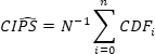
where Δ̃adj denotes the adjusted slope heterogeneity test statistic; N represents the number of cross-sectional units; T denotes the number of time periods; k is the number of explanatory variables; and S̃ represents the standardized Swamy slope dispersion statistic used to evaluate parameter heterogeneity across panel units. Finally, stationarity was evaluated using the Cross-sectionally Augmented Im–Pesaran–Shin (CIPS) unit root test, which accommodates both cross-sectional dependence and heterogeneous slope coefficients41:
 (6)
(6)
where CIPS denotes the Cross-sectionally Augmented Im–Pesaran–Shin panel unit root statistic; N represents the number of cross-sectional units; CDFi denotes the cross-sectionally augmented Dickey–Fuller statistic for the ith cross-sectional unit; and i indexes the individual cross-sectional units. The results of these diagnostic tests guided the selection of second-generation panel econometric techniques suitable for heterogeneous panel datasets.
Panel cointegration test
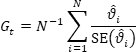
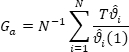
To determine whether a stable long-run equilibrium relationship exists among renewable energy capacity, environmental policy performance, greenhouse gas emissions, eco-friendly technology, and Green GDP, the Panel ARDL bounds cointegration test was employed. Compared with conventional residual-based cointegration tests, the Westerlund approach accommodates cross-sectional dependence, heterogeneous slope coefficients, and small sample sizes. The test produces four statistics: two group-mean statistics (Gt and Ga) and two panel statistics (Pt and Pa). Rejection of the null hypothesis indicates the presence of a long-run equilibrium relationship among the variables36,42:
 (7a)
(7a)
 (7b)
(7b)
 (7c)
(7c)
 (7d)
(7d)
where Gt and Ga denote the group-mean test statistics of the Panel ARDL bounds cointegration test; Pt and Pa denote the panel test statistics; N represents the number of cross-sectional units; T denotes the number of time periods;  is the estimated error-correction coefficient for the ith cross-sectional unit;
  represents the pooled error-correction coefficient; SE() and SE() denote the corresponding standard errors; and i indexes the individual cross-sectional units. The presence of cointegration justifies estimating long-run elasticities and subsequent quantile-based analyses.
Method of moments quantile regression (MMQR)
Because conventional panel estimators provide only average effects, they may conceal substantial heterogeneity across countries operating at different levels of renewable energy deployment. To capture these heterogeneous effects, the Method of Moments Quantile Regression (MMQR) was employed.
MMQR estimates the effects of ecological policy performance, greenhouse gas emissions, eco-friendly technology, and Green GDP across multiple conditional quantiles of renewable energy capacity, thereby allowing the influence of explanatory variables to vary according to the maturity of renewable energy deployment. The method simultaneously accounts for individual fixed effects and unobserved heterogeneity while estimating both location and scale parameters43:
 (8)
(8)
where Qτ(Yit | Xit) denotes the conditional τth quantile of the dependent variable; Yit represents renewable energy capacity (REC); Xit denotes the vector of explanatory variables (EPI, GHG emissions, EFT, and Green GDP); σ1 is the intercept; ζ is the vector of location parameters; αi represents the country-specific fixed effect; Zit denotes the scale covariates; γ is the vector of scale parameters; Uit is the error term; and i and t index countries and years, respectively. The scale component of the MMQR model is specified as follows43:
 (9)
(9)
where Zi(X) denotes the scale function of the explanatory variables; Zi represents the vector of scale covariates; X denotes the vector of explanatory variables; i indexes the cross-sectional units (countries); and k denotes the total number of explanatory variables. As a robustness analysis, a conventional panel quantile regression with bootstrapped standard errors was also estimated to verify the consistency of the MMQR findings.
Panel causality test
The direction of causal relationships among renewable energy capacity, ecological policy performance, greenhouse gas emissions, eco-friendly technology, and Green GDP was examined using the Dumitrescu–Hurlin panel Granger non-causality test44. This approach accommodates cross-sectional dependence and heterogeneous panel structures while identifying whether causal relationships are unidirectional or bidirectional.
The panel causality analysis complements the cointegration and MMQR analyses by distinguishing between variables that drive renewable energy capacity and those that respond to changes in renewable energy deployment. Establishing causal direction provides additional evidence to inform policy prioritization and the sequencing of renewable energy interventions.
All statistical analyses were performed using statistical analysis software. The analytical sequence, from diagnostic testing and cointegration analysis to quantile regression and panel causality testing, provides a coherent and reproducible framework for evaluating the determinants of renewable energy capacity across OECD countries.
Access restricted. Please log in or start a trial to view this content.
Results
Descriptive statistics
The distributional characteristics of the study variables were examined before econometric estimation. Table 2 summarizes the descriptive statistics for the log-transformed variables across 21 OECD countries during 2000–2020. Renewable energy capacity (REC), ecological performance index (EPI), greenhouse gas (GHG) emissions, eco-friendly technology (EFT), and Green GDP exhibited substantial cross-country and temporal variation, with standard deviations ...
Access restricted. Please log in or start a trial to view this content.
Discussion
The present study examined the determinants of renewable energy capacity across 21 OECD countries during 2000–2020 by integrating environmental policy performance, greenhouse gas (GHG) emissions, eco-friendly technology (EFT), and Green GDP within a Method of Moments Quantile Regression (MMQR) framework. The findings reveal substantial heterogeneity in the conditional distribution of renewable energy capacity, indicating that the effects of environmental, technological, and economic factors vary with countries'...
Access restricted. Please log in or start a trial to view this content.
Disclosures
All authors declare no conflicts of interest.
Acknowledgements
This work is supported by the Philosophy and Social Science Research Project of Jiangsu Provincial Department of Education (2022SJYB2268).
Access restricted. Please log in or start a trial to view this content.
Materials
| Name | Company | Catalog Number | Comments |
|---|---|---|---|
| CIPS unit root test | StataCorp | Stata 18 | Implemented using the xtcips or multipurt command for the Cross-sectionally Augmented Im-Pesaran-Shin panel unit root test. |
| Cross-sectional dependence (CD) test | StataCorp | Stata 18 | Implemented using the xtcsd command to perform the Pesaran CD test. |
| Dumitrescu–Hurlin panel Granger non-causality test | StataCorp | Stata 18 | Implemented using the xtgcause command for panel causality analysis. |
| Eco-friendly technology (EFT) | OECD Statistics | N/A | Data on environment-related patent applications retrieved from the OECD Statistics database (https://stats.oecd.org/). |
| Ecological Performance Index (EPI) | OECD Statistics | N/A | Data retrieved from the OECD Statistics database (https://stats.oecd.org/). |
| EViews | IHS Global Inc. | Version 14 | Alternative statistical analysis software for panel econometrics. |
| Green GDP | World Bank | N/A | Data retrieved from the World Bank DataBank (https://databank.worldbank.org/). Specifically, data on Adjusted Net Savings, which is used to calculate Green GDP. |
| Greenhouse gas (GHG) emissions | OECD Statistics | N/A | Data retrieved from the OECD Statistics database (https://stats.oecd.org/). |
| Method of Moments Quantile Regression (MMQR) | StataCorp | Stata 18 | Implemented using the mmqreg command, which must be installed from the Statistical Software Components (SSC) archive. |
| Pesaran–Yamagata slope heterogeneity test | StataCorp | Stata 18 | Implemented using the xttest3 or xthetero command. |
| R | R Foundation | Version 4.6.0 or higher | Open-source alternative for statistical computing. |
| Renewable energy capacity (REC) | OECD Statistics | N/A | Data retrieved from the OECD Statistics database (https://stats.oecd.org/). |
| Stata | StataCorp | Version 18 | Primary software used for all statistical analyses, including diagnostic testing, cointegration, quantile regression, and panel causality tests. |
| Westerlund panel cointegration test | StataCorp | Stata 18 | Implemented using the xtwest command, which must be installed from the SSC |
References
- Hassan Q, et al. The renewable energy role in the global energy Transformations. Renewable Energy Focus. 2024 Mar 1;48:100545.
- Wang Z, et al. The transition of renewable energy and ecological sustainability through environmental policy stringency: Estimations from advanced panel estimators. Renew Energy. 2022;188:70-80.
- Zhang D, Kong Q. Green energy transition and sustainable development of energy firms: An assessment of renewable energy policy. Energy Econ. 2022;111:106060.
- Zhou X, et al. Transition to renewable energy and environmental technologies: The role of economic policy uncertainty in the top five polluted economies. J Environ Manage. 2022;313:115019.
- Ullah S, Luo R, Nadeem M, Cifuentes-Faura J. Advancing sustainable growth and energy transition in the United States through the lens of green energy innovations, natural resources and environmental policy. Resour Policy. 2023;85:103848.
- Yin HT, Wen J, Chang CP. Going green with artificial intelligence: The path of technological change toward the renewable energy transition. Oecon Copernicana. 2023;14(4):1059-1095.
- Niaz MS, Khoso AK, Talpur KR, Talpur BA. Beyond the curve: How economic complexity and pandemics reshape the energy-emissions nexus in Asia. IEEE Access. 2026;14:22946-22957.
- Rabbani MR, Kiran M. Financing the future: Insights into sustainable energy investments through scientific mapping and meta-analysis. Discov Sustain. 2025;6(1):34.
- Obrero EJ, Mohamed N. The nexus between carbon pricing, clean fuel technology, and renewable energy sources: implications for carbon emission reduction. Climate Economics and Social Impact (CESI). 2023;1(1):55-67.
- Sahoo M, Sethi N, Padilla MA. Unpacking the dynamics of information and communication technology, control of corruption, and sustainability in green development in developing economies: New evidence. Renew Energy. 2023;216:119088.
- Liu H, Zhu Q, Khoso WM, Khoso AK. Spatial pattern and the development of green finance trends in China. Renew Energy. 2023;211:370-378.
- Behera B, Sucharita S, Patra B, Sethi N. A blend of renewable and non-renewable energy consumption on economic growth in India: The role of disaggregate energy sources. Environ Sci Pollut Res. 2024;31(3):3902-3916.
- Sabbar SS. An econometric analysis of the causes of environmental degradation in developing countries. Climate Economics and Social Impact (CESI). 2023;1(1):24-38.
- Saleh HM, Hassan AI. The challenges of sustainable energy transition: A focus on renewable energy. Appl Chem Eng. 2024;7(2):2084.
- Rabbani MR, Kiran M. The nexus of FinTech, environmental sustainability, and climate change: Insights from OIC emerging economies. Sustain Futures. 2025;10:100986.
- Javed A, et al. Do green technology innovation, environmental policy, and the transition to renewable energy matter in times of ecological crises? A step toward ecological sustainability. Technol Forecast Soc Change. 2024;207:123638.
- Omri A, Jabeur SB. Climate policies and legislation for renewable energy transition: The roles of the financial sector and political institutions. Technol Forecast Soc Change. 2024;203:123347.
- Das A, Sethi N. Modelling the environmental pollution-institutional quality nexus in low- and middle-income countries: Exploring the role of financial development and educational level. Environ Dev Sustain. 2023;25(2):1492-1518.
- Ghaffar A, Sardar M. Different regions' climate vulnerability and the success of transitioning to renewable energy. Climate Economics and Social Impact (CESI). 2023;1(1):39-54.
- Liza FF, et al. Environmental technology development and renewable energy transition toward carbon-neutrality goals in G20 countries. Clean Technol Environ Policy. 2024;26(10):3369-3390.
- Ivanovski K, Marinucci N. Policy uncertainty and renewable energy: Exploring the implications for global energy transitions, energy security, and environmental risk management. Energy Res Soc Sci. 2021;82:102415.
- Jain S, Puri N, Rabbani MR. Dynamic interconnectedness and risk transmission in green, clean energy, and sustainable markets. Indian J Finance. 2025;29-48.
- Sun G, Li G, Dilanchiev A, Kazimova A. Promotion of green financing: The role of renewable energy and energy transition in China. Renew Energy. 2023;210:769-775.
- Behera P, et al. Pathways to achieve carbon neutrality in emerging economies: Catalyzing the role of renewable energy, green growth, information and communication technology, and political risk. Renew Energy. 2025;243:122514.
- Wei S, Jiandong W, Saleem H. The impact of renewable energy transition, green growth, green trade, and green innovation on environmental quality: Evidence from the top 10 green future countries. Front Environ Sci. 2023;10:1076859.
- Chen B, Xiong R, Li H, Sun Q, Yang J, et al. Pathways for sustainable energy transition. J Clean Prod. 2019;228:1564-1571.
- Jacobsson S, Lauber V. The politics and policy of energy system transformation: Explaining the German diffusion of renewable energy technology. Energy Policy. 2006;34(3):256-276.
- Esiri AE, Kwakye JM, Ekechukwu DE, Benjamin O. Public perception and policy development in the transition to renewable energy. Magna Sci Adv Res Rev. 2023;8(2):228-237.
- Pradhan P, et al. Can green growth and ecological footprint mitigation go hand in hand? The role of sectoral energy consumption, green innovation, and greenfield investment in emerging economies. Econ Change Restruct. 2025;58(2):18.
- Kilinc-Ata N, Çamkaya S. Assessing the impact of technology on the European Union clean energy transition: Evidence from the Green Energy Mix Quality Index. Int J Energy Sect Manag. 2026;20(4):1068-1087.
- Li Y, et al. Geopolitical risks and the global renewable energy transition: Implications for energy security and economic resilience. Energy Rep. 2026;15:108875.
- Li B. The role of financial markets in the energy transition: An analysis of investment trends and opportunities in renewable energy and clean technology. Environ Sci Pollut Res. 2023;30(43):97948-97964.
- Sethi L, et al. Sustainable future orientation for BRICS+ nations: Green growth, political stability, renewable energy, and technology for ecological footprint mitigation. Renew Energy. 2025;244:122701.
- Pesaran MH, Schuermann T, Weiner SM. Modeling regional interdependencies using a global error-correcting macroeconometric model. J Bus Econ Stat. 2004;22(2):129-162.
- Behera P, Sethi L, Saqib N, Sethi N. Green finance and public-private partnerships: Dynamic ARDL insights into renewable energy and air quality enhancement. Econ Change Restruct. 2026;59(1):16.
- Westerlund J. Testing for error correction in panel data. Oxf Bull Econ Stat. 2007;69(6):709-748.
- Zhang X, Feng D, Wang J, Sui A. Integrating renewable energy systems: Assessing financial innovation, renewable energy generation intensity, energy transition, and environmental regulation with renewable energy sources. Energy Strateg Rev. 2024;56:101567.
- Asante D, et al. Renewable energy technology transition among small- and medium-scale firms in Ghana. Renew Energy. 2021;178:549-559.
- Kaya Y. Impact of carbon dioxide emission control on GNP growth. Energy and Industry Subgroup, Response Strategies Working Group, Intergovernmental Panel on Climate Change (IPCC). Paris, France. 1990.
- Pesaran MH, Yamagata T. Testing slope homogeneity in large panels. J Econometrics. 2008;142(1):50-93.
- Pesaran MH. A simple panel unit root test in the presence of cross-section dependence. J Appl Econom. 2007;22(2):265-312.
- Chudik A, Pesaran MH, Shin Y. Long-run effects in large heterogeneous panel data models with cross-sectionally correlated errors. Adv Econ. 2016;36:85-135.
- Machado JAF, Silva JMC. Quantiles via moments. J Econometrics. 2019;213(1):145-173.
- Dumitrescu EI, Hurlin C. Testing for Granger non-causality in heterogeneous panels. Econ Model. 2012;29(4):1450-1460.
- Behera B, Behera P, Sucharita S, Sethi N. Mitigating ecological footprint in BRICS countries: Unveiling the role of disaggregated clean energy, green technology innovation, and political stability. Discov Sustain. 2024;5(1):165.
- Omri A, Hamza F, Alkahtani N. When do innovation and renewable energy transition drive environmental sustainability? Sustainability. 2025;17(15):6910.
- Jiang Y, Guo Y, Bashir MF, Shahbaz M. Do renewable energy, environmental regulations, and green innovation matter for China's zero-carbon transition? Evidence from green total factor productivity. J Environ Manage. 2024;352:120030.
- Behera B, et al. Fuelling the low-carbon transportation sector in emerging economies: Role of institutional quality, environmental tax, green technology innovation, and biofuel. Transp Policy. 2025;166:124-134.
- Osei A, Osei Agyemang A, Kofi Boadi P. Navigating the path to ecological sustainability in MENA's green transition: The role of renewable energy adoption and environmental regulation. Manage Environ Qual. 2025;36(6):1352-1371.
- Zhong J, Kan HY. The impact of government policy, natural resources, and ecological innovations on energy transition and environmental sustainability: Insights from China. Resour Policy. 2024;89:104531.
- Behera P, Behera B, Sethi N, Handoyo RD. What drives environmental sustainability? The role of renewable energy, green innovation, and political stability in OECD economies. Int J Sustain Dev World Ecol. 2024;31(7):761-775.
- Sethi L, Behera P, Behera B, Sethi N. Unravelling the role of renewable energy, information and communication technology, and agricultural credit for sustainable agricultural productivity in developing countries. Int J Sustain Dev World Ecol. 2024;31(7):989-1003.
Access restricted. Please log in or start a trial to view this content.
Reprints and Permissions
This article has been published
Video Coming Soon