Blockchain-Integrated Bidirectional Long Short-Term Memory Network for Real-Time Intrusion Detection in Healthcare Internet of Medical Things

Summary

This protocol describes the implementation of a blockchain-integrated bidirectional long short-term memory intrusion detection system for healthcare Internet of Medical Things networks, enabling real-time attack detection, tamper-proof forensic logging, and automated mitigation.

Abstract

Healthcare Internet of Medical Things (IoMT) environments require intrusion detection systems that not only identify cyberattacks accurately but also provide forensic accountability, auditability, and rapid response capabilities. Conventional intrusion detection approaches primarily emphasize classification performance while offering limited support for tamper-proof event recording and post-incident investigation. This study presents a forensic-aware intrusion detection framework that integrates an Extended Bidirectional Long Short-Term Memory (BiLSTM) network with a permissioned blockchain layer to support real-time detection, secure logging, and automated mitigation in healthcare IoMT systems. The protocol combines data preprocessing, AQU-IMF-RFE feature selection, temporal sequence modeling, attention-based learning, residual connections, and blockchain-based event recording. The Extended BiLSTM model was trained and evaluated independently on the UNSW-NB15, CICIDS2017, and Bot-IoT benchmark datasets using reproducible preprocessing, stratified data partitioning, and fixed random seeds. Intrusion events detected by the model were recorded on a Proof-of-Authority blockchain through smart contracts that enabled immutable logging and automated response actions. Experimental results demonstrated high intrusion detection performance with low false-positive rates across all evaluated datasets while maintaining forensic traceability and real-time response capability. The blockchain layer provided tamper-resistant audit records and automated mitigation without introducing prohibitive computational overhead. These findings demonstrate that integrating deep-learning-based intrusion detection with blockchain-enabled forensic logging improves the trustworthiness, accountability, and practical deployability of healthcare cybersecurity systems.

Introduction

In the healthcare system, digitization has led to a new era of intelligent, connected, and patient-centered healthcare services. Modern medical infrastructure heavily relies on network communication and data exchange between wearable sensors, remote patient monitoring systems, electronic health records (EHRs)^1,2, and intelligent diagnostic platforms. However, this increasing interconnectivity also expands the attack surface of healthcare networks, exposing them to cyber threats such as data breaches, ransomware, distributed denial-of-service (DDoS) attacks, and man-in-the-middle attacks³. These intrusions result in substantial financial losses and, more importantly, can jeopardize patient safety when sensitive medical data or critical device functionality is compromised.

The scale and complexity of Internet of Medical Things (IoMT) systems further exacerbate these security challenges. Modern healthcare networks must simultaneously provide low-latency communication, high reliability, and robust security guarantees, requirements that traditional security mechanisms often struggle to satisfy⁴. The rapid growth of IoMT traffic, characterized by heterogeneous data sources, dynamic communication patterns, and stringent regulatory requirements such as the Health Insurance Portability and Accountability Act (HIPAA) and the General Data Protection Regulation (GDPR), necessitates intelligent intrusion detection systems (IDSs) capable of achieving high detection rates while minimizing false alarms⁵.

In regulated healthcare environments, intrusion detection is not merely an operational requirement but also an accountability function. Security alerts may trigger device isolation, affect continuity of care, and subsequently become subject to audits, regulatory reviews, or legal investigations. Consequently, an effective IoMT IDS must provide accurate real-time detection, explainable decisions that support incident triage, and tamper-proof records that ensure non-repudiation and forensic traceability⁶. This requirement shifts the objective of intrusion detection from performance-centric classification toward trust-centric and accountability-driven security governance.

Deep learning techniques, particularly Long Short-Term Memory (LSTM) and Bidirectional Long Short-Term Memory (BiLSTM) networks, have demonstrated strong capability in modeling temporal dependencies within network traffic and detecting anomalous behavior⁷. Nevertheless, existing BiLSTM-based IDSs frequently suffer from overfitting, insufficient attention to critical temporal events, and limited generalization across heterogeneous IoMT devices and healthcare environments. Furthermore, IoMT networks are exposed to a diverse range of cyber threats that affect the Confidentiality, Integrity, and Availability (CIA) of medical data and services, as summarized in Table 1.

Attack Type	IoMT Context	CIA Dimension Affected	Impact on Healthcare Systems
Unauthorized Access19	Exploitation of weak authentication mechanisms to access patient devices or medical records	Confidentiality, Integrity	Data leakage and unauthorized control of medical devices
Spoofing / Impersonation19	Malicious device mimics a legitimate IoMT node	Integrity	False readings that may lead to misdiagnosis or unsafe treatment
Eavesdropping21	Interception of unencrypted medical data during transmission	Confidentiality	Privacy breaches and exposure of sensitive patient information
Data Tampering / Firmware Exploits19	Modification of device firmware or transmitted healthcare data	Integrity	Incorrect diagnosis or inappropriate therapy decisions
Ransomware20	Encryption of patient data or medical-device firmware	Availability, Integrity	Lockout of critical systems and treatment delays
Denial-of-Service (DoS) / Distributed Denial-of-Service (DDoS)6	Overloading medical devices or healthcare networks	Availability	Service disruption affecting monitoring systems and intensive care unit (ICU) operations
Side-Channel Attacks22	Extraction of cryptographic keys through timing or power-analysis techniques	Confidentiality	Device compromise and cryptographic key theft

Table 1: Common cyberattacks affecting Internet of Medical Things healthcare environments. This table summarizes representative cyberattacks that target Internet of Medical Things (IoMT) systems, their operational context, the affected Confidentiality, Integrity, and Availability (CIA) security dimensions, and their potential impact on healthcare delivery, patient safety, and medical-device operation.

Blockchain technology offers several advantages that can complement intrusion detection in IoMT environments. As summarized in Table 2, blockchain enables immutable event logging for forensic validation, facilitates automated mitigation through smart contracts, removes single points of failure through decentralized operation, and supports compliance with healthcare data protection regulations by maintaining traceable audit trails. Despite these benefits, blockchain-based security mechanisms remain underutilized in healthcare IDSs.

Feature	Description	Benefits in Healthcare Context
Data Integrity	Each transaction is cryptographically hashed and linked to the previous block	Ensures immutability of patient and device records
Tamper Detection	Any modification to stored data changes the block hash and invalidates the chain	Enables rapid detection of unauthorized record modification
Access Control	Smart contracts enforce predefined permissions and authorization policies	Restricts access to sensitive healthcare information to authorized users and devices
Data Provenance	Each event is digitally signed and time-stamped	Supports forensic traceability, auditing, and regulatory compliance
Low-Latency Consensus	Proof-of-Authority (PoA) consensus mechanism enables rapid transaction validation with lower computational overhead than Proof-of-Work	Supports near real-time event logging in critical healthcare environments

Table 2: Benefits of blockchain technology for healthcare Internet of Medical Things intrusion detection systems. This table summarizes key blockchain features and their associated benefits in healthcare Internet of Medical Things (IoMT) environments. The listed capabilities support immutable logging, tamper detection, access control, data provenance, and low-latency consensus mechanisms required for secure and auditable intrusion detection.

Beyond performance evaluation, blockchain integration provides protection against multiple security threats in IoMT environments. Table 3 summarizes the strengths and limitations of blockchain in this context, highlighting threats that are effectively mitigated, such as data tampering and repudiation, and threats that require additional safeguards. The blockchain layer supports low-latency logging suitable for real-time healthcare environments, Byzantine resilience against faulty or malicious nodes, and scalability across distributed hospital networks and IoMT devices.

Security Threat	Addressed by Blockchain?	Mechanism	Notes
Data Tampering27	Yes	Cryptographic hash linking	Any modification invalidates chain integrity
Repudiation26	Yes	Digital signatures associated with each block	Prevents denial of recorded intrusion events
Centralized Failure25	Yes	Distributed ledger maintained across authorized gateways	Eliminates a single point of failure
Sybil Attack24	Partial	Permissioned PoA consensus requiring trusted validators	Can be mitigated through identity-based validator authorization
51% Attack23	Partial	Requires compromise of a majority of authorized validators	Less likely in private PoA blockchain deployments
Data Provenance26	Yes	Time-stamped and digitally signed event records	Supports forensic traceability and regulatory compliance

Table 3: Security threats addressed by blockchain integration in healthcare Internet of Medical Things environments. This table summarizes major security threats relevant to Internet of Medical Things (IoMT) systems and indicates the extent to which blockchain technology mitigates each threat. The underlying protection mechanisms and implementation considerations are provided for each threat category.

Most existing IDSs rely on predefined rules or lightweight machine-learning models^8,9. Although such approaches can identify known attack patterns, they often struggle to cope with the dynamic and evolving nature of modern cyber threats. They are particularly inadequate for securing rapidly growing IoMT-based healthcare infrastructures, where false alarms, limited adaptability, and poor auditability can significantly affect operational efficiency. Rule-based systems frequently generate high false-positive rates because they cannot reliably distinguish benign anomalies from genuine attacks⁹. Conventional machine-learning models trained on static or outdated datasets, as well as existing deep learning-based intrusion detection approaches, often fail to generalize emerging attack behaviors, including zero-day intrusions^10,11. In addition, traditional centralized logging approaches remain vulnerable to tampering, thereby limiting the reliability of post-incident forensic investigations¹². Many existing IDS solutions also impose substantial computational overhead, making them difficult to deploy on resource-constrained IoMT devices and gateways¹³. As a result, healthcare IoMT environments remain vulnerable to sophisticated, multistage cyberattacks. Addressing these challenges requires an intelligent, secure, and resource-efficient intrusion detection framework capable of learning temporal traffic patterns in real time while simultaneously ensuring forensic trustworthiness and automated mitigation of detected threats.

Despite significant advances in machine learning and deep learning–based intrusion detection, several critical gaps remain. First, many existing IDS models are developed and evaluated using static datasets and therefore lack adaptability to continuously evolving attack behaviors. Second, although advanced deep learning architectures can improve detection accuracy, they often provide limited interpretability and fail to prioritize clinically important traffic patterns. Third, and most importantly, current IDS frameworks generally do not provide intrinsic support for forensic trustworthiness, auditability, or immutable record keeping, capabilities that are essential for regulatory compliance, incident investigation, and legal accountability in healthcare systems.

While blockchain-based logging mechanisms provide data integrity and transparency, they are rarely integrated cohesively with advanced deep learning-based intrusion detection models in latency-sensitive IoMT environments. Existing studies typically focus either on improving detection performance without addressing forensic integrity or on blockchain-based security mechanisms without incorporating advanced temporal anomaly detection. Consequently, a significant gap remains in developing a unified framework capable of simultaneously delivering real-time spatio-temporal intrusion detection, tamper-proof forensic logging, automated mitigation, and practical deployment within heterogeneous and resource-constrained healthcare IoMT environments.

Motivated by these challenges, this study aims to develop an intrusion detection framework that enhances BiLSTM networks through attention mechanisms and custom layers for improved temporal feature prioritization, integrates blockchain technology for secure and verifiable intrusion logging and automated response, and operates efficiently in real-time healthcare IoMT settings. We hypothesize that integrating an attention-enhanced Extended BiLSTM architecture with blockchain-based forensic logging and automated mitigation mechanisms will improve intrusion detection effectiveness while simultaneously providing the auditability, trustworthiness, and accountability required in regulated healthcare environments.

This work addresses a fundamental gap in IoMT security research by treating intrusion detection as a forensic accountability problem rather than solely as a classification problem. The proposed framework integrates artificial intelligence (AI)-driven detection, immutable event recording, and automated response mechanisms into a unified architecture that supports clinical safety, regulatory compliance, and operational trust. The increasing adoption of IoMT devices and cloud-connected healthcare infrastructures has made healthcare networks attractive targets for cyberattacks, including ransomware, data manipulation, unauthorized access, and denial-of-service attacks that threaten the confidentiality, integrity, and availability of patient information. The proposed Extended BiLSTM–Blockchain framework establishes a closed-loop security process that connects attack detection directly to forensic validation and automated mitigation.

The principal contributions of this study are fivefold. First, a clinically aligned temporal intrusion detection model is developed by extending a conventional BiLSTM architecture with dual-directional temporal learning, residual connections, attention mechanisms, and custom layers to improve the detection of complex attack patterns in healthcare network traffic. Second, a lightweight blockchain-based security layer is integrated with the Extended BiLSTM model to provide immutable, secure, and tamper-proof logging of intrusion events and system actions. Third, an end-to-end real-time IDS pipeline is developed for healthcare environments, enabling live traffic analysis and intrusion prediction with low latency and high accuracy. Fourth, the proposed framework is comprehensively evaluated using three publicly available benchmark datasets, namely UNSW-NB15, CICIDS2017, and Bot-IoT. Finally, the architecture is designed as a scalable and extensible edge-cloud framework suitable for practical deployment in healthcare networks, medical infrastructures, and e-health applications.

By combining the temporal learning capabilities of Extended BiLSTM networks with the trust and immutability provided by blockchain technology, the proposed framework delivers a secure and trustworthy IDS tailored to the evolving cybersecurity requirements of healthcare environments. The framework bridges critical gaps in healthcare network security and establishes a foundation for broader adoption of AI and blockchain integration in protecting critical healthcare infrastructures.

Protocol

All experiments were conducted exclusively using publicly available benchmark network intrusion datasets (UNSW-NB15, CIC-IDS-2017, and Bot-IoT), which contain network traffic records without identifiable personal or medical information. The datasets were used in accordance with their respective licenses and terms of use. Because no human participants, patient samples, or identifiable personal data were involved, institutional ethics approval and informed consent were not required.

Overview of the Proposed Framework
This section presents the proposed dual-layer intrusion detection and prevention framework for securing IoMT environments. The framework integrates an Extended BiLSTM network for spatio-temporal intrusion detection with a lightweight blockchain layer for tamper-proof logging and automated mitigation. Unlike conventional IDS approaches that focus solely on detection accuracy, the proposed architecture is designed to simultaneously support real-time detection, forensic accountability, and regulatory compliance, which are essential requirements in healthcare systems. The overall workflow and architecture of the proposed Extended BiLSTM–Blockchain intrusion detection framework for IoMT networks are illustrated in Figure 1.

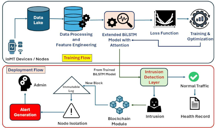
Figure 1. Architecture of the proposed Extended BiLSTM–Blockchain intrusion detection framework for Internet of Medical Things networks. Schematic representation of the proposed framework showing the training and deployment workflows. In the training workflow, Internet of Medical Things (IoMT) devices generate network traffic that undergoes data preprocessing and feature engineering before being analyzed by the Extended Bidirectional Long Short-Term Memory (BiLSTM) model with temporal attention. Model parameters are optimized through loss-function computation and iterative training. In the deployment workflow, the trained model performs intrusion detection according to the decision function defined in Equation 13. Detected intrusion events are forwarded to the blockchain module, where immutable logging, node isolation, and administrator alert generation are performed. BiLSTM, Bidirectional Long Short-Term Memory; IoMT, Internet of Medical Things. Please click here to view a larger version of this figure.

IoMT devices generate heterogeneous data streams consisting of network traffic, device metadata, and patient-related signals. Such raw inputs are often noisy, redundant, and inconsistent, making them unsuitable for direct model training. Therefore, a preprocessing pipeline is applied to ensure the quality and structure of the data before feeding it into the Extended BiLSTM model. The detailed preprocessing pseudocode is provided in Algorithm 1 (Supplementary File 1), which outlines the preprocessing pipeline applied to IoMT data streams prior to Extended BiLSTM training (pseudocode in Supplementary File 1; implementation in Supplementary File 2). The complete Extended BiLSTM architecture is summarized in Algorithm 2 (Supplementary File 1).

End-to-End Reproduction Workflow
The full study can be reproduced using the steps below. Software and hardware are listed in the Experimental Setup, and the supplementary code covers each step.

Get the datasets → Download UNSW-NB15. Use the files UNSW_NB15_training-set.csv and UNSW_NB15_testing-set.csv. Download CICIDS2017. Use the five MachineLearningCSV day files (Monday to Friday). Download Bot-IoT. Use the 5% subset files UNSW_2018_IoT_Botnet_Full5pc_1_to_4. Earlier intrusion detection studies commonly relied on benchmark datasets such as KDD Cup 99¹⁴; however, this study uses the more recent UNSW-NB15, CICIDS2017, and Bot-IoT datasets to better represent contemporary network traffic. Process each dataset separately. The UNSW-NB15 dataset is available from the University of New South Wales at https://research.unsw.edu.au/projects/unsw-nb15-dataset (last modified: February 8, 2024). The CICIDS2017 dataset is available from the Canadian Institute for Cybersecurity at https://www.unb.ca/cic/datasets/ids-2017.html (released: July 2017). The Bot-IoT dataset is available from the University of New South Wales at https://research.unsw.edu.au/projects/bot-iot-dataset (last modified: February 5, 2024). All datasets were accessed in May 2025 for this study.

Preprocess the data → Remove corrupted records. Fill missing values using training-set means. Apply EMA denoising (α = 0.3). Normalize features to [0,1] using training-set statistics. Label-encode categorical fields. Build sliding windows (T = 20, stride = 1). These preprocessing steps support robust intrusion detection by reducing noise and improving the quality of network traffic representations for machine-learning-based IDSs^15,16.

Select features (AQU-IMF-RFE) → Rank features by mutual information. Refine with the Aquila Optimizer. Apply Random Forest RFE with 10-fold cross-validation. Keep the final features. This hybrid feature-selection strategy follows the broader concept of combining complementary intrusion detection techniques¹⁷ and is implemented using the AQU-IMF-RFE framework developed in our previous work¹⁸.

Train the model → For each dataset, the data were randomly partitioned into training (80%) and testing (20%) sets using a fixed random seed of 42. Twenty percent of the training partition was further reserved as the validation set. Build the Extended BiLSTM. Train using weighted binary cross-entropy loss and the Adam optimizer (learning rate = 0.001, batch size = 64, maximum of 50 epochs, with early stopping). Save the trained model. The use of temporal deep-learning models is well suited to heterogeneous IoMT traffic¹⁹. The complete model-training workflow is summarized in Algorithm 3 (Supplementary File 1). The final class weights were computed automatically from the training-set class distributions according to Equations 19 and 20. The resulting class weights were as follows: UNSW-NB15: , ; CICIDS2017: , ; and Bot-IoT (5% subset): , . The large value of w_n for the Bot-IoT dataset reflects the severe underrepresentation of benign samples in the training partition of the 5% subset.

Deploy the blockchain → Start the Proof-of-Authority (PoA) chain. Deploy the smart contract and note its address. Authorize the gateway accounts. Run the client so that each detected intrusion is logged and triggers isolation and alerts. The complete detection, blockchain logging, and mitigation workflow is summarized in Algorithm 4 (Supplementary File 1). The blockchain layer was implemented using the go-ethereum (Geth) client version 1.13.15 to operate the permissioned PoA network, the Solidity compiler (solc) version 0.8.19 for smart-contract compilation and deployment, and the web3.py library version 6.15.1 for communication between the IDS and the blockchain network.

Evaluate → Test the model on the held-out test set. Compute accuracy, precision, recall, F1-score, and false-positive rate. Record latency and throughput. Verify the integrity of the blockchain ledger. The complete evaluation workflow is summarized in Algorithm 5 (Supplementary File 1). Detection latency (T_d) was measured from immediately before the model inference call to the time at which the predicted probabilities were returned. End-to-end mitigation latency (T_d + T_b) was measured from the same starting point until completion of the corresponding blockchain block-creation transaction. Throughput was calculated as the total number of preprocessed test windows processed by the complete detection-and-logging pipeline divided by the elapsed wall-clock time required for a single complete pass through each dataset’s test set. The workload consisted of the windowed test partitions while preserving the original benign-to-intrusion class distribution. Malicious windows additionally incurred the blockchain-logging overhead, whereas benign windows incurred only the intrusion-detection cost.

Generate figures and tables → Plot the accuracy and loss curves, confusion matrix, and comparative evaluation charts. Build the comparison tables. The complete figure and table generation workflow is summarized in Algorithm 6 (Supplementary File 1). The complete custom-developed source code used to generate all figures and tables is provided in Supplementary File 2. In particular, the figures.py script reproduces the manuscript figures directly from the saved experimental outputs (e.g., training history and confusion-matrix files), while the remaining scripts generate the processed data and performance metrics used to construct the reported tables.

Figure 2 is the implementation-level data flow between the IDS and blockchain modules. The Extended BiLSTM produces a per-window decision (Equation 13); on a malicious classification, the gateway client constructs and signs a transaction and submits it over web3/JSON-RPC to the PoA smart contract, which appends a hash-linked block (Equation 14) to the immutable ledger and emits events (BlockCreated, NodeIsolated, and AdminAlert) that trigger node isolation and administrator alerts.

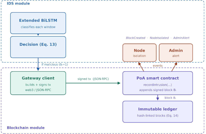
Figure 2. Implementation-level interaction between intrusion detection and blockchain modules. Workflow diagram illustrating communication between the intrusion detection system and blockchain components. The Extended BiLSTM model classifies each input window and applies the decision rule defined in Equation 13. When an intrusion is detected, the gateway client generates and signs a transaction that is transmitted through Web3.py/JSON-RPC to the Proof-of-Authority (PoA) smart contract. The contract appends a hash-linked block to the immutable ledger according to Equation 14 and emits BlockCreated, NodeIsolated, and AdminAlert events that trigger containment and notification actions. IDS, Intrusion Detection System; BiLSTM, Bidirectional Long Short-Term Memory; PoA, Proof-of-Authority; JSON-RPC, JavaScript Object Notation–Remote Procedure Call. Please click here to view a larger version of this figure.

Data Representation
Let’s consider R as the raw IoMT traffic stream. After preprocessing, each raw record  is mapped into a normalized d-dimensional feature vector (Equation 1):

 (1)

Here, f (⋅) is the feature transformation function mapping raw records into a d dimensional normalized feature vector. Let the IoMT network consist of a set of nodes (Equation 2):

N = {n₁ , n₂, ... , n_k} (2)

Each node n_j ∈ R produces a time-series data stream (Equation 3):

  (3)

Here, x_t is the feature vector at time t, with d features (e.g., packet size, protocol type, source/destination address) commonly observed in Internet of Things healthcare network traffic¹⁹. The corresponding label set is (Equation 4):

  (4)

Here, y_t=0 represents normal traffic and y_t =1 denotes an intrusion.

Data Preprocessing
The preprocessing pipeline includes the following steps, which address common data-quality and security challenges associated with IoMT traffic²⁰:

Data Cleaning and Missing-Value Handling:
A record was identified as corrupted and removed prior to imputation if it satisfied either of the following explicit conditions: (i) all feature fields in the record were missing (i.e., the entire record was null), or (ii) the record contained a non-finite value (positive or negative infinity) in any numeric field after type coercion. The second rule removes invalid entries such as those produced by division-by-zero during flow-feature computation (for example, infinite flow-rate values arising from zero-duration flows). After corrupted records were removed, remaining missing values were imputed by mean replacement computed per feature, per dataset, and from the training partition only; the resulting means were applied to the training, validation, and test sets to prevent information leakage. Imputation was not class-conditional, and means were not pooled across datasets.

Temporal Denoising:
Temporal denoising was performed using a per-feature exponential moving average (EMA) filter applied along the time axis. The recursive (causal) form y_t = α·x_t + (1 − α)·y_t−1 was used, with smoothing factor α = 0.3, implemented via the pandas ewm function with adjust=False. Each feature was smoothed independently. As an exponential (infinite-impulse-response) filter, the EMA has no fixed window or kernel size; the smoothing factor α is the single parameter governing the degree of smoothing and the effective memory of the filter.

Min–Max Normalization:
Min–max normalization was applied to scale each feature to the [0,1] range using the transformation x′=(x−min)/(max−min+ε), where ε = 1 × 10⁻⁸. The minimum and maximum statistics were computed per feature, per dataset, and from the training partition only; these stored training statistics were then applied to normalize the training, validation, and test sets, preventing leakage of held-out information. During inference, feature values falling outside the training range were clipped to the [0,1] interval.

Encoding of Categorical Features:
Categorical features were converted to numeric form using label encoding. This was applied to all categorical variables: in UNSW-NB¹⁵, the proto, service, and state fields; in Bot-IoT, the proto field; CICIDS2017 contains no categorical fields among the selected features. Encoding was implemented with LabelEncoder fitted per variable.

Temporal Windowing for Sequential Learning:
The preprocessed feature stream was segmented into fixed-length sequences using a sliding window of length T = 20 time steps with a stride of s = 1. Each generated window was validated before inclusion. A window was accepted only if it contained exactly T = 20 consecutive time steps and all feature values were finite. Streams shorter than T = 20 records produced no windows. This configuration (T = 20, s = 1, 95% overlap) was applied consistently across all experiments and datasets. The complete preprocessing workflow is summarized in Algorithm 1 (Supplementary File 1).

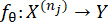
The goal of preprocessing is to enable a predictive mapping from input sequences to intrusion labels (Equation 5).

   (5)

parameterized by θ, that predicts whether an event is benign or malicious.

Feature Selection Using AQU-IMF-RFE
Feature selection was performed using AQU-IMF-RFE, a hybrid method that integrates Mutual Information (MI), the Aquila Optimizer (AO), and Recursive Feature Elimination (RFE), introduced in our prior work¹⁸. The method operates in three stages. In the first stage, the mutual information between each feature and the class label is computed to obtain an initial relevance ranking. In the second stage, the Aquila Optimizer performs a global search over candidate feature subsets using its four optimization strategies. In the third stage, the refined subset is passed through Recursive Feature Elimination with 10-fold cross-validation using a Random Forest (RF) estimator.

The Aquila Optimizer was configured with a population size of 100, a maximum of 10 iterations, an exploitation factor of 0.1, a learning rate of 0.1, and an attraction factor of 0.005. Applied independently to each dataset, AQU-IMF-RFE retained 14 features for UNSW-NB15, 24 for CICIDS2017, and 12 for Bot-IoT. The complete pseudocode is provided in Supplementary File 1, and the selected feature subsets are listed in Table 4.

Table 4A. Selected Features Retained for UNSW-NB15
S. No.	Feature	Type	Category
1	dur	Numeric (float)	Basic
2	sbytes	Numeric (integer)	Basic
3	rate	Numeric (float)	Basic
4	dload	Numeric (float)	Basic
5	sinpkt	Numeric (float)	Time
6	dinpkt	Numeric (float)	Time
7	sjit	Numeric (float)	Time
8	tcprtt	Numeric (float)	Time
9	synack	Numeric (float)	Time
10	ackdat	Numeric (float)	Time
11	smean	Numeric (integer)	Content
12	ct_srv_src	Numeric (integer)	Connection
13	ct_dst_src_ltm	Numeric (integer)	Connection
14	ct_srv_dst	Numeric (integer)	Connection
Table 4B. Selected Features Retained for CICIDS2017
S. No.	Feature
1	Destination Port
2	Flow Duration
3	Total Length of Forward Packets
4	Total Length of Backward Packets
5	Forward Packet Length Maximum
6	Backward Packet Length Maximum
7	Backward Packet Length Mean
8	Flow Packets
9	Flow Inter-Arrival Time Maximum
10	Forward Inter-Arrival Time Total
11	Forward Header Length
12	Backward Header Length
13	Forward Packets per Second
14	Maximum Packet Length
15	Packet Length Mean
16	Packet Length Standard Deviation
17	Packet Length Variance
18	Average Packet Size
19	Average Backward Segment Size
20	Subflow Forward Bytes
21	Subflow Backward Bytes
22	Initial Window Bytes Forward
23	Initial Window Bytes Backward
24	Forward Packet Length Mean
Table 4C. Selected Features Retained for Bot-IoT
S. No.	Feature	Type
1	seq	Numeric
2	mean	Numeric
3	stddev	Numeric
4	min	Numeric
5	max	Numeric
6	srate	Numeric (float)
7	drate	Numeric (float)
8	N_IN_Conn_P_SrcIP	Numeric (integer)
9	N_IN_Conn_P_DstIP	Numeric (integer)
10	proto	Categorical (encoded)
11	state_number	Numeric (integer)
12	rate	Numeric (float)

Table 4: Features selected by the AQU-IMF-RFE feature-selection method. This table lists the final feature subsets selected by the AQU-IMF-RFE feature-selection framework for the UNSW-NB15, CICIDS2017, and Bot-IoT datasets. Feature names, data types, and functional categories are provided where applicable.

Experimental Setup
All experiments were conducted on a Dell PowerEdge R740 server equipped with an Intel Xeon Silver 4214 processor operating at a base frequency of 2.20 GHz, with 12 physical cores, 24 logical threads, 16.5 MB cache, and an Intel Ultra Path Interconnect (UPI) speed of 9.6 GT/s. The server was configured with 128 GB RAM, a 512 GB solid-state drive (SSD), and operated on Microsoft Windows 11. The software stack comprised Python 3.12.7, TensorFlow 2.16.1, scikit-learn 1.8.0, pandas 3.0.2, and NumPy 2.4.4. The blockchain layer was implemented on the same workstation using a PoA Ethereum network. Communication between the IDS and the blockchain was performed via JSON-RPC using the go-ethereum (Geth) client version 1.13.15, the Solidity compiler (solc) version 0.8.19 for smart-contract compilation and deployment, and the Web3.py library version 6.15.1. Reported training time, inference latency, and throughput were measured on this hardware and software configuration.

Model Architecture and Training
The Extended BiLSTM model constitutes the core detection component of the framework, building upon previous learning-based intrusion detection approaches developed for IoMT environments²¹. Earlier intrusion detection studies highlighted both the importance of balancing detection performance with false-alarm reduction¹⁵ and the unique challenges of applying machine-learning methods to evolving network traffic¹⁶. Collaborative neural-network intrusion detection architectures have further demonstrated the value of deep sequential feature learning for complex network traffic²². While standard BiLSTM models capture bidirectional temporal dependencies, IoMT traffic exhibits both short-term burst patterns and long-range dependencies caused by multistage attacks. To address this, the proposed model extends BiLSTM with temporal feature extraction, enhanced bidirectional temporal learning, residual connections, and attention-based temporal prioritization. Bidirectional LSTMs (BiLSTM) overcome this limitation by combining forward and backward hidden states, enabling richer temporal representation of IoMT traffic patterns, as given in Algorithm 2 (Supplementary File 1).

Let the input sequence be X^(n_j) = {x₁ , x₂ , ... , x_T }, where each x_t ∈ R^d is a preprocessed feature vector.

Temporal Feature Extraction:
A lightweight one-dimensional convolution is applied across the time dimension to emphasize short-range temporal anomalies (Equation 6):

U = φ (Conv1D(X^(n_j)), U = {u₁, u₂, ..., u_T }   (6)

Here, φ(⋅) is a nonlinear activation function and the convolved features u_t are fed to the BiLSTM.

The Conv1D layer extracts short-range temporal patterns before bidirectional sequence modeling. Complete implementation parameters are provided in Supplementary File 3B.

Stacked Bidirectional LSTM Learning:
Forward and backward hidden states are computed as (Equation 7):

  (7)

The final BiLSTM representation is the concatenation of past (forward) and future (backward) hidden states (Equation 8).

   (8)

Two stacked BiLSTM layers model bidirectional temporal dependencies. Detailed architectural parameters are provided in Supplementary File 3B. Weight initialization details are provided in Supplementary File 3B.

Residual Connection and Normalization
After linear projection to matching dimensions, residual connections and layer normalization are applied (Equation 9):

Residual projection and layer normalization align the convolutional and BiLSTM feature representations before attention. Detailed implementation parameters are provided in Supplementary File 3B.

Attention Mechanism
Although BiLSTM provides strong temporal modeling, not all time steps contribute equally to the prediction. To emphasize critical timestamps (e.g., sudden anomalous spikes), an attention mechanism is introduced. Each hidden state  is assigned a relevance score α_t to enhance detection accuracy (Equation 10).

Here, W_a is a trainable parameter and the attention weights satisfy 

The context vector c aggregates the hidden states based on their learned importance (Equation 11):

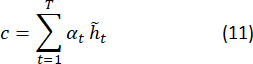
The attention mechanism aggregates temporal representations into a context vector. Detailed implementation parameters are provided in Supplementary File 3B.

Output Layer and Classification
The aggregated context vector is passed through a fully connected layer followed by a sigmoid activation to yield the final prediction (Equation 12):

Here, W_c and b_c are trainable parameters, and σ(·) is the sigmoid activation function mapping the output to the interval [0,1]. A threshold is applied to classify traffic as benign () or intrusive ().

Dropout regularization and the fixed classification threshold used during inference are described in Supplementary File 3B.

The Extended BiLSTM architecture is identical across the three datasets; only the input feature dimension differs, taking values of 14, 24, and 12 for UNSW-NB15, CICIDS2017, and Bot-IoT, respectively. Because the Conv1D layer maps any -dimensional input to a fixed 64-channel representation, all subsequent layers are independent of the dataset, and only the input shape and the Conv1D parameter count vary with . The complete layer-by-layer architecture is summarized in Table 5, with parameter counts expressed in terms of d; the resulting totals are 184,641, 186,561, and 184,257 trainable parameters for d = 14, d = 24, and d = 12, respectively.

S. No.	Layer (Type)	Output Shape	Trainable Parameters	Activation Function
1	Input	(20, d)	0	—
2	Conv1D (64 filters, kernel size = 3, same padding)	(20, 64)	192d + 64	ReLU
3	Bidirectional LSTM Layer 1 (64 units per direction)	(20, 128)	66,048	tanh / sigmoid
4	Bidirectional LSTM Layer 2 (64 units per direction)	(20, 128)	98,816	tanh / sigmoid
5	Dense Residual Projection	(20, 128)	8,320	Linear
6	Residual Addition	(20, 128)	0	—
7	Layer Normalization (axis = −1, ε = 1 × 10⁻³)	(20, 128)	256	—
8	Temporal Attention (Wa ∈ ℝ¹²⁸×¹)	128	128	Softmax
9	Dense Hidden Layer	64	8,256	ReLU
10	Dropout (p = 0.3)	64	0	—
11	Dense Output Layer	1	65	Sigmoid

Table 5: Layer-by-layer architecture of the Extended Bidirectional Long Short-Term Memory model. This table summarizes the architecture of the proposed Extended Bidirectional Long Short-Term Memory (BiLSTM) model, including layer types, output dimensions, trainable parameter counts, and activation functions.

The software and computational environment used for all experiments is summarized in Table 6.

Component	Version / Specification
Operating System	Windows
Server Platform	Dell PowerEdge
CPU	64-core processor
RAM	128 GB
Storage	512 GB SSD
Python	3.12.7
NumPy	2.4.4
pandas	3.0.2
scikit-learn	1.8.0
TensorFlow / Keras	2.16.1
web3 (blockchain client)	6.15.1
eth-account	0.1
Solidity Compiler (solc)	0.8.19
go-ethereum (Geth)	1.13.15

Table 6: Software and computational environment used for implementation and evaluation of the proposed framework. This table summarizes the hardware specifications, software components, blockchain tools, and version numbers used for data preprocessing, feature selection, model training, blockchain deployment, and performance evaluation.

Intrusion Decision and Automated Response
Intrusion detection in healthcare environments is only effective if followed by rapid response and mitigation. The Intrusion Detection Layer converts the predicted probability into a decision. Formally, the intrusion decision at time step t is represented as follows (Equation 13):

Here,  is the predicted intrusion probability at time t and  is the classification threshold.

Once an intrusion is detected, the Intrusion Detection Layer interfaces directly with the blockchain module, which performs immutable logging, automated mitigation, and closed-loop security enforcement. Event details, including source information, destination information, and selected traffic features, are recorded in a new blockchain block. Smart contracts execute real-time mitigation actions such as node isolation and administrator alerts. This closed-loop architecture allows intrusion detection results to feed directly into prevention mechanisms, thereby minimizing mitigation latency. Thus, the Intrusion Detection Layer serves as the bridge between temporal detection using the Extended BiLSTM model and secure response using blockchain technology, completing the end-to-end functionality of the proposed framework.

Blockchain-Based Forensic Logging
While the Extended BiLSTM model enables real-time intrusion detection, secure storage and verifiable auditing of intrusion events are equally critical in IoMT healthcare environments. Traditional centralized logging mechanisms are vulnerable to tampering and compromise forensic traceability. To address this limitation, the proposed framework incorporates a lightweight blockchain module that ensures immutability, decentralization, and smart-contract-based automated response.

Each detected intrusion event generates a block that is added to the blockchain. A block B_i is defined as follows (Equation 14):

Here, H_i is the cryptographic hash of the event data, timestamp, and prediction result, T_i is the timestamp, D_i contains selected intrusion-event features, Si_gi is the digital signature, and PrevHash links the block to the previous block, ensuring immutability.

This design guarantees tamper resistance because any modification of D_i or T_i changes the block hash and breaks chain integrity. It also provides auditability because all detected anomalies are permanently stored and verifiable. Automated mitigation is supported through smart contracts that execute predefined actions such as node isolation and administrator alerts. Decentralization is achieved through multiple IoMT gateways maintaining the distributed ledger, thereby eliminating a single point of failure.

Block generation uses the Keccak-256 cryptographic hash function, the native hashing primitive of the Ethereum/Solidity environment (invoked through Solidity’s keccak256). For each intrusion block, the block hash is computed as follows:

Here, D_i is the event feature digest, T_i is the timestamp, and PrevHash is the hash of the preceding block. The fields are concatenated using Solidity's tightly packed encoding (abi.encodePacked) before hashing, producing a 256-bit digest.

The same Keccak-256 computation is used by the chain-verification routine, which recomputes each block hash from its stored fields and confirms that it matches the recorded value, thereby validating chain integrity. Keccak-256 was selected because it is the standard collision-resistant hashing algorithm used natively within Ethereum smart contracts. The smart contract was developed in Solidity and compiled using the Solidity compiler (solc) version 0.8.19. It was deployed on a private Ethereum Proof-of-Authority (PoA) network operated using Geth version 1.13.15. The blockchain network was configured with four validator nodes using the Clique Proof-of-Authority consensus protocol, a chain ID of 9848, a block period of 5 s, and a block gas limit of 30,000,000. Communication between the Extended BiLSTM intrusion detection engine and the blockchain layer was implemented using the Web3.py library version 6.15.1 through the HTTP JSON-RPC interface.

PoA Consensus Mechanism
Because healthcare IoMT systems are highly latency sensitive, the proposed framework employs a PoA consensus mechanism instead of computationally expensive Proof-of-Work (PoW)²³. In PoA, a fixed set of trusted validator nodes, such as hospital gateways, authorize transactions, providing both efficiency and resilience.

The time complexity of block validation under PoW can be expressed as follows (Equation 15):

Here, d represents mining difficulty.

In contrast, the time complexity of PoA consensus is given as follows (Equation 16):

because validation only requires digital-signature verification by authorized validator nodes.

As a result, PoA provides low-latency operation suitable for real-time medical alerts, energy efficiency by avoiding computationally intensive mining, and resilience against a limited number of malicious validators. The PoA network was configured with four validator nodes, and this configuration was kept fixed throughout all experiments to ensure consistent latency measurements, reproducible performance evaluation, and fair comparison across all benchmark datasets.

Blockchain Implementation and Smart-Contract Operation
The blockchain component was implemented on a permissioned Ethereum network operating under the PoA consensus model²⁴. The network was run using the go-ethereum (Geth) client with the Clique PoA consensus protocol²⁵, in which a set of authorized validator (sealer) nodes are responsible for producing and validating blocks. The intrusion-logging smart contract (IoMTIntrusionLedger) was written in Solidity and deployed to this network, following blockchain-based IoT security architectures for secure decentralized event management²⁶. Only gateway accounts authorized on-chain (via the contract’s access-control function) were permitted to submit intrusion records, consistent with permissioned blockchain smart-contract architectures for Internet of Things applications²⁷. The blockchain layer was implemented using the go-ethereum (Geth) client version 1.13.15 for operating the permissioned PoA network, the Solidity compiler (solc) version 0.8.19 for smart-contract compilation and deployment, and the Web3.py library version 6.15.1 for communication between the IDS and the blockchain network.

Detailed blockchain deployment and configuration parameters are provided in Supplementary File 3C.

Each intrusion record is digitally signed before being committed to the ledger, supporting blockchain-based healthcare auditability and secure forensic record keeping²⁸. Digital signature generation and verification procedures, including ECDSA over the secp256k1 curve^29,30, are described in Supplementary File 3D. Each gateway holds an Ethereum key pair consisting of a 256-bit (32-byte) private key and the corresponding public key, from which its account address is derived; key generation follows the standard Ethereum procedure, using a cryptographically secure random 256-bit private key with the public key obtained by secp256k1 scalar multiplication. To create a signature, the gateway client computes the event feature digest D_i and signs it with its private key using the EIP-191 message-signing format, producing a 65-byte signature consisting of the r, s, and v components. The signature is submitted together with the intrusion record. Verification is performed on-chain by the smart contract: using the EVM ecrecover precompile, the contract recovers the signer's address from the signed digest and signature and requires it to equal the address of the authorized gateway submitting the transaction. If the recovered address does not match an authorized gateway, the transaction is rejected. This binds every ledger entry to a specific authorized gateway and prevents unauthorized or forged intrusion records.

Smart contracts are triggered automatically upon intrusion detection , ensuring real-time response without requiring manual intervention (Equation 17):

  (17)

The blockchain module operates in parallel with the Extended BiLSTM classifier. Once an anomaly is detected: (i) the event is labeled and classified by the BiLSTM, (ii) a block is generated, signed, and appended to the blockchain ledger, and (iii) smart contracts enforce automatic response policies.

The intrusion-logging smart contract (IoMTIntrusionLedger) maintains an append-only ledger of intrusion blocks and a registry of authorized gateway accounts, and it exposes the functions summarized in Table 7. The contract enforces two access roles through modifiers: onlyAdmin (the deploying administrator) and onlyGateway (accounts authorized to submit intrusion records). State consists of the gateway authorization mapping, the block ledger array, and the current chain head (the hash of the most recent block).

S. No.	Function / Component	Type	Access	Logic
1	constructor	Constructor	—	Sets the deployer as the administrator and authorizes it as the initial gateway.
2	setGateway(address, bool)	Function	onlyAdmin	Adds or removes an authorized gateway account; emits GatewayUpdated.
3	recordIntrusion(nodeId, patientId, attackClass, probabilityBp, dataDigest, signature, isolate)	Function	onlyGateway	Computes Hi = Keccak-256(Di ∥ Ti ∥ probability ∥ PrevHash); verifies the gateway's ECDSA signature on Di via ecrecover; appends the block to the ledger; advances the chain head; emits BlockCreated, optionally NodeIsolated, and AdminAlert. Returns Hi.
4	verifyChain()	View Function	Public	Recomputes every block's hash from its stored fields and checks the PrevHash linkage; returns true only if the entire chain is consistent (tamper detection).
5	ledgerLength()	View Function	Public	Returns the number of blocks in the ledger.
6	_recoverSigner(hash, sig)	Internal Function	—	Splits the 65-byte signature into (r, s, v) and recovers the signing address via the ecrecover precompile.
7	BlockCreated / NodeIsolated / AdminAlert / GatewayUpdated	Events	—	Emitted for off-chain listeners to drive logging, node isolation, administrator alerts, and gateway-registry updates.
8	onlyAdmin / onlyGateway	Modifiers	—	Restrict functions to the administrator and to authorized gateways, respectively.

Table 7: Functions, events, and access-control components of the IoMTIntrusionLedger smart contract. This table summarizes the principal functions, events, and access-control modifiers implemented within the permissioned blockchain smart contract. These components support gateway authorization, intrusion logging, blockchain verification, event generation, and automated mitigation.

The immutability property of the blockchain directly follows from Equation 14, where any modification to event data or timestamps invalidates the hash chain. Blockchain thus provides data integrity, traceability, and auditability for healthcare systems through immutable forensic records. Patient and device intrusion records remain unchanged once stored, each block securely links to the previous block enabling chronological event reconstruction, and healthcare administrators or regulators can verify intrusion incidents without risk of falsification.

Loss Function and Model Optimization
The proposed Extended BiLSTM model addresses the binary classification problem of distinguishing between normal traffic and intrusion events in IoMT networks. To guide the training process, a binary cross-entropy (BCE) loss is adopted, which is well suited for probabilistic outputs from the sigmoid activation layer. For a dataset with N samples, the loss is defined as follows (Equation 18):

  (18)

Here,  is the ground-truth label of the i^th input sequence (0 = benign, 1 = intrusion), and  is the predicted probability of intrusion.

The framework operates as a two-stage classification pipeline. The first stage performs binary intrusion detection: the Extended BiLSTM produces a sigmoid output  and applies the threshold τ = 0.5 to classify each window as benign or intrusive (Equations 12,13), trained with weighted binary cross-entropy loss. A second stage can perform attack categorization, in which windows identified as intrusions are passed to a multiclass classifier that assigns the specific attack category using a softmax output layer trained with categorical cross-entropy. The present study focuses on and evaluates the binary detection stage. The two stages share the same Extended BiLSTM feature-extraction backbone (Conv1D, BiLSTM, residual, normalization, and attention layers); they differ only in their output layer (sigmoid for detection and softmax for categorization) and corresponding loss function. The binary detection stage and the multiclass categorization stage were trained and evaluated under the same data partitions, random seed, and training conditions described above.

While IoMT traffic is often imbalanced, a weighted binary cross-entropy loss is used to penalize misclassification of the minority class. Class weights are computed using the number of intrusion samples N_p, the number of benign samples N_n, and the total number of samples N (Equations 19,20):

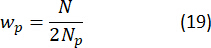
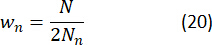
The weighting ensures that the model is not biased toward the dominant benign traffic class and remains sensitive to rare but critical intrusion events.

The weighted binary cross-entropy loss is given as follows (Equation 21):

  (21)

Training was performed using mini-batches of size 64. At the start of every epoch, the training samples were randomly shuffled before being partitioned into batches so that batch composition varied across epochs and the model did not see examples in a fixed order. Batches were not explicitly balanced or stratified by class; instead, each batch reflected the natural class distribution of the training set, and class imbalance was addressed through the class-weighted binary cross-entropy loss (Equations 19–21). The validation subset reserved from the training partition remained fixed across epochs and was not shuffled into the training batches.

The class weights in the weighted binary cross-entropy loss were not set manually but were computed automatically for each dataset from its training-set class counts according to Equations 19 and 20. For the UNSW-NB15 dataset, the resulting class weights were  for the normal class and  for the intrusion class. For the CICIDS2017 dataset, the resulting class weights were  for the normal class and  for the intrusion class. For the Bot-IoT dataset (5% subset), the resulting class weights were  for the normal class and  for the intrusion class.

Training Strategy and Optimization
The Extended BiLSTM model was trained using mini-batches of size B = 64 with weighted binary cross-entropy loss, the Adam optimizer, and early stopping based on validation loss. Training was capped at 50 epochs, and early stopping was applied with patience K = 5. If validation loss did not improve for five consecutive epochs, training was halted and the model weights were restored to those from the epoch with the lowest validation loss. Thus, 50 epochs represented the maximum training budget rather than a fixed training duration. A dropout probability of 0.3 was applied for regularization. The architectural settings included 64 Conv1D filters, 64 LSTM units per direction, a window length of T = 20, and a stride of s = 1. The adopted training strategy is summarized in Algorithm 3 (Supplementary File 1). The Adam update equations used for optimization are provided in Supplementary File 3A.

The Adam optimizer was configured with a learning rate of , a first-moment decay rate (β₁) of 0.9, a second-moment decay rate (β₂) of 0.999, and a numerical-stability constant () of 1 × 10^-7. No additional optimizer options were used, and no weight decay or gradient clipping was applied.

Alert Generation and Automated Mitigation
Detection alone is insufficient in latency-sensitive IoMT networks, where rapid response is critical to ensure patient safety. The Alert Generation and Mitigation Layer operationalizes the intrusion decision made by the Extended BiLSTM model and the blockchain logging mechanism. If δ_t = 1, the blockchain module appends a new block containing the intrusion details . Simultaneously, a smart contract is executed to trigger mitigation actions (Equation 22):

  (12)

Here, BlockCreation ensures immutable forensic logging of the event, NodeIsolation (n_j) quarantines the compromised IoMT node to prevent further damage, and AdminAlert delivers real-time notification to system administrators. To operate this dual-layer response pipeline, the pseudocode is presented in Algorithm 4 (Supplementary File 1).

Smart-contract event processing and off-chain response mechanisms are described in Supplementary File 3E.

Each entry committed to the blockchain ledger is stored as an IntrusionBlock record, whose fields and data formats are listed in Table 8. The ledger is an append-only array of these records, and the current chain head stores the hash of the most recently added block.

S. No.	Field	Data Type	Size	Description
1	hashId	bytes32	32 bytes	Block hash Hi = Keccak-256(Di ∥ Ti ∥ probability ∥ PrevHash)
2	timestamp	uint256	32 bytes	Block creation time Ti (Unix epoch seconds, from the block timestamp)
3	nodeId	bytes32	32 bytes	Identifier of the IoMT node nj
4	patientId	bytes32	32 bytes	Patient/device identifier (forensic metadata)
5	attackClass	uint16	2 bytes	Attack-category code (0 = Normal, 1 = DDoS, 2 = Spoofing, ...)
6	probabilityBp	uint16	2 bytes	Predicted intrusion probability ŷ in basis points (0–10000, i.e. 0.00–100.00%)
7	dataDigest	bytes32	32 bytes	Digest Di of the selected event features
8	signature	bytes	Variable (65 bytes)	ECDSA signature Sigi of the event digest by the gateway (r, s, v)
9	prevHash	bytes32	32 bytes	Hash of the previous block (PrevHash), linking the chain
10	isolated	bool	1 byte	Whether node isolation was triggered for this record

Table 8: Structure of the IntrusionBlock record stored in the blockchain ledger. This table describes the fields, data types, storage sizes, and purposes of the blockchain ledger records used to store intrusion events. The structure supports cryptographic integrity verification, forensic traceability, and automated response mechanisms.

The overall mitigation latency can be expressed as the sum of the detection delay (T_d) from the Extended BiLSTM model and the blockchain execution delay (T_b) (Equation 23):

   (23)

Computational Complexity Analysis
The efficiency of the proposed Extended BiLSTM–Blockchain framework is determined by both the computational cost of the BiLSTM model and the overhead introduced by the blockchain module. The proposed framework integrates Extended BiLSTM detection with blockchain logging to satisfy the core security requirements of the Confidentiality, Integrity, and Availability (CIA) triad.

Let the preprocessed input sequence length be T, the feature dimension be d, and the hidden dimension of the BiLSTM be h.

For each time step, a BiLSTM processes input of dimension d with hidden size h. Since it is bidirectional (forward + backward) (Equation 24):

) (24)

Here, T is sequence length (time steps), d is input feature dimension, h is hidden state dimension

The attention layer computes importance weights and aggregates hidden states with complexity (Equation 25).

  (25)

which is linear in both the sequence length T and hidden dimension h.

The overall detection complexity per sequence is therefore given as follows (Equation 26):

  (26)

demonstrating that temporal modeling dominates the computational cost, while the attention mechanism introduces only a lightweight overhead.

For each detected intrusion event, blockchain logging performs hashing, signing, and block-appending operations (Equation 27):

   (27)

For N intrusion-detection events, the combined complexity becomes as follows (Equation 28):

 (28)

which can be simplified as follows (Equation 29):

  (29)

because the blockchain overhead grows linearly with the number of events and remains negligible compared with sequence-processing computations.

Computational complexity is summarized in Equations 24–29. Detailed interpretation is provided in Supplementary File 3F.

Results

The results are organized to mirror the methodological steps of the Protocol, with each subsection reporting the observations produced by the corresponding step.

Dataset handling and experimental setup
The three benchmark datasets were analyzed independently rather than merged. Because UNSW-NB15, CICIDS2017, and Bot-IoT use different feature schemas and labeling conventions, each dataset was preprocessed, windowed, and evaluated separately using its own 80:20 train/test split. The Extended BiLSTM model was trained and tested on each dataset independently, and the performance metrics (accuracy, precision, recall, and F1-score) are reported separately for each dataset. This independent evaluation protocol avoids feature-space inconsistencies that would arise from combining heterogeneous datasets and enables the robustness of the proposed framework to be assessed across three distinct network environments.

The proposed Extended BiLSTM-BC model was trained and evaluated using preprocessed normal and malicious traffic extracted from the CICIDS2017, UNSW-NB15, and Bot-IoT datasets. The data were partitioned using a single stratified hold-out split. The UNSW-NB15 dataset provides predefined training and testing partitions, which were used directly in this study. For the remaining two datasets (CICIDS2017 and Bot-IoT), the preprocessed windowed samples were divided into training and test sets using an 80:20 split with stratified random sampling (scikit-learn train_test_split, stratified by class label), thereby preserving the benign-to-intrusion class ratio across the partitions. Within the training set, an additional 20% was reserved for validation (Keras validation_split), resulting in an effective 64% training, 16% validation, and 20% test partition. The validation set was used for early stopping. A fixed random seed of 42 was applied to scikit-learn, NumPy, and TensorFlow to support reproducibility. The Extended BiLSTM network was optimized using the Adam optimizer with a learning rate of 0.001, a batch size of 64, and a maximum of 50 training epochs.

Feature selection results
Prior to model training, feature selection was performed independently for each dataset using AQU-IMF-RFE, an Aquila Optimizer (AO)-guided Recursive Feature Elimination procedure in which candidate features were ranked according to their mutual information (MI) with the class label and iteratively eliminated while the Aquila Optimizer searched for the optimal feature subset. Identifier fields (e.g., flow IDs, IP addresses, and port numbers) and textual attack-category fields were excluded before feature selection to prevent information leakage. This procedure retained 14 features for UNSW-NB15, 24 features for CICIDS2017, and 12 features for Bot-IoT. The complete list of selected input variables, their data types, and their source datasets is provided in Table 4, and an expanded description of each feature is included in Supplementary File 2.

Training and convergence
During training, the model demonstrated stable convergence, with both training and validation performance improving as the network parameters approached their optimal values. The layer-by-layer architecture of the proposed Extended BiLSTM model is summarized in Table 5, while the software and computational environment used for implementation and evaluation are presented in Table 6. The blockchain smart-contract functions supporting intrusion logging and automated mitigation are summarized in Table 7, and the structure of the blockchain intrusion record is presented in Table 8. The complete set of training hyperparameters used in this study is summarized in Table 9, supporting the reproducibility of the proposed framework.

Training Hyperparameter	Value
Learning Rate	0.001
Optimizer	Adam
Batch Size	64
Maximum Epochs	50
Output Activation Function	Sigmoid
Train-test split	80:20, stratified
Validation split	20% of the training partition
Random seed	42
Input window length	20 time steps
Sliding-window stride	1
Conv1D filters	64
Conv1D kernel size	3
Conv1D padding	Same
Conv1D activation	ReLU
BiLSTM layers	2
BiLSTM units	64 units per direction
BiLSTM output dimension	128
LSTM activation	Tanh
Residual projection dimension	128
Early-stopping patience	5 epochs
Dense hidden-layer units	64
Dense hidden-layer activation	ReLU
Dropout rate	0.3
Output units	1
Classification threshold	0.5
Loss Function	Weighted Binary Cross-Entropy (WBCE)

Table 9: Hyperparameter configuration used for training the Extended Bidirectional Long Short-Term Memory model. This table lists the principal training hyperparameters used during development of the Extended Bidirectional Long Short-Term Memory (BiLSTM) intrusion detection model, including optimization settings, activation function, batch size, training duration, and loss function.

Table 10 presents the training and validation accuracies of the proposed model over 50 epochs, recorded at 5-epoch intervals. The model showed rapid improvement during the first 10 epochs, achieving training and validation accuracies of 96.0% and 95.5%, respectively. Beyond epoch 20, the accuracy gains became incremental, and both curves converged closely. By epoch 50, the model stabilized at 99.1% training accuracy and 98.5% validation accuracy, indicating minimal overfitting and strong generalization performance. The corresponding learning curve is shown in Figure 3, illustrating the progression of training and validation accuracy throughout the optimization process.

Epoch	Training Accuracy (%)	Validation Accuracy (%)
1	72.1	70
5	90	89
10	96	95.5
15	97.1	96.5
20	97.8	97.2
25	98.2	97.5
30	98.5	97.8
35	98.7	98
40	98.9	98.2
45	99	98.4
50	99.1	98.5

Table 10: Training and validation accuracy during Extended Bidirectional Long Short-Term Memory model training. This table reports training and validation accuracy measured at selected training epochs during optimization of the Proposed Extended Bidirectional Long Short-Term Memory (BiLSTM) model. These values were used to generate the accuracy convergence curve shown in Figure 3.

Figure 3. Training and validation accuracy of the Extended BiLSTM model. Line plot showing classification accuracy during model training. The x-axis represents training epochs (1–50), and the y-axis represents classification accuracy (%). Blue circles indicate training accuracy, and orange squares indicate validation accuracy. Please click here to view a larger version of this figure.

Table 11 presents the training and validation loss values recorded at the same 5-epoch intervals. During the initial training phase, the training loss decreased from 0.64 to 0.28, while the validation loss decreased from 0.67 to 0.31 by epoch 5. After epoch 20, the rate of loss reduction became more gradual, and both curves converged steadily. By epoch 50, the training loss stabilized at 0.08, whereas the validation loss remained close at 0.12, indicating only a small difference between the two curves. This convergence reflects effective optimization, limited overfitting, and good generalization to previously unseen data. The corresponding training and validation loss curves are presented in Figure 4. The computational efficiency of the evaluated models, including inference latency and throughput, is summarized in Table 12. Detailed analysis of these measurements is presented later in the Computational efficiency subsection.

Epoch	Training Loss	Validation Loss
1	0.64	0.67
5	0.28	0.31
10	0.13	0.17
15	0.11	0.15
20	0.1	0.14
25	0.095	0.13
30	0.09	0.125
35	0.085	0.122
40	0.083	0.12
45	0.082	0.118
50	0.08	0.12

Table 11: Training and validation loss during Extended Bidirectional Long Short-Term Memory model training. This table reports training and validat  ion weighted binary cross-entropy loss values measured at selected training epochs during optimization of the Proposed Extended Bidirectional Long Short-Term Memory (BiLSTM) model. These values were used to generate the loss convergence curve shown in Figure 4.

Figure 4. Training and validation loss of the Extended BiLSTM model. Line plot showing weighted binary cross-entropy loss during model training. The x-axis represents training epochs (1–50), and the y-axis represents loss values. Blue circles indicate training loss, and orange squares indicate validation loss. Please click here to view a larger version of this figure.

Model	Latency (Averaged ms/event)	Throughput (Averaged events/s)
Decision Tree	40	845
Support Vector Machine	75	670
LSTM	110	559
Proposed Extended BiLSTM–Blockchain Framework	135	320

Table 12: Latency and throughput comparison of intrusion detection models. This table compares inference latency and processing throughput among representative machine-learning and deep-learning intrusion detection models. Latency is reported as milliseconds per event and throughput is reported as processed events per second.

Detection performance
Table 13 presents the comparative evaluation of the proposed framework against conventional ML and DL baseline models across the three benchmark datasets. The proposed model achieved accuracies of 98.9% on CICIDS2017, 95.9% on UNSW-NB15, and 98.8% on Bot-IoT, together with high sensitivities of 96.9%, 97.6%, and 98.8%, respectively. On CICIDS2017 and UNSW-NB15, the proposed model attained the highest accuracy among all evaluated models, whereas on Bot-IoT it achieved the highest accuracy (98.8%), matched by the Decision Tree (DT) baseline. On Bot-IoT, the proposed model slightly outperformed the LSTM baseline (98.3%) and performed comparably to the Support Vector Machine (SVM) baseline (98.7%); the smaller performance margins on this dataset reflect its extreme class imbalance, in which benign traffic constitutes only a very small fraction of the test set. Overall, the proposed model maintained a strong balance between sensitivity and precision, demonstrating robust intrusion-detection performance across all datasets while providing the most reliable assessment on the more balanced benchmark datasets (CICIDS2017 and UNSW-NB15). The corresponding comparisons of accuracy, precision, and recall across datasets and baseline models are presented in Figures 5–7.

Dataset	Model	Sensitivity (%)	Specificity (%)	Accuracy (%)	Precision (%)	Recall (%)
CICIDS2017	Proposed Extended BiLSTM–Blockchain	96.9	99.4	98.9	97.5	96.9
	LSTM	93.3	98.5	97.5	93.9	93.3
	SVM	94.8	98.8	98.1	95.1	94.8
	DT	93.1	98.7	97.5	94.6	93.1
UNSW-NB15	Proposed Extended BiLSTM–Blockchain	97.6	93.9	95.9	95.1	97.6
	LSTM	95.2	88.5	92.2	91.1	95.2
	SVM	96.5	91.1	94.1	93.1	96.5
	DT	96.9	92.2	94.8	93.8	96.9
Bot-IoT	Proposed Extended BiLSTM–Blockchain	98.8	90.5	98.8	99.3	98.8
	LSTM	98.3	89.4	98.3	99.2	98.3
	SVM	98.7	88.4	98.7	99.3	98.7
	DT	98.8	93.6	98.8	99.3	98.8

Table 13: Performance comparison of intrusion detection models across benchmark datasets. This table compares the proposed framework and baseline intrusion detection models on the CICIDS2017, UNSW-NB15, and Bot-IoT datasets using sensitivity, specificity, accuracy, precision, and recall performance metrics.

Figure 5. Accuracy comparison across datasets and machine learning/deep learning models. Grouped bar chart comparing classification accuracy (%) obtained by different models across the CICIDS2017, UNSW-NB15, and Bot-IoT datasets. Bars represent the proposed model, Long Short-Term Memory (LSTM), Support Vector Machine (SVM), and Decision Tree (DT). The x-axis represents datasets, and the y-axis represents classification accuracy (%). Please click here to view a larger version of this figure.

Figure 6. Precision comparison of classification models across intrusion detection datasets. Grouped bar chart showing precision (%) obtained by different models on the CICIDS2017, UNSW-NB15, and Bot-IoT datasets. The x-axis represents classification models, and the y-axis represents precision (%). LSTM, Long Short-Term Memory; SVM, Support Vector Machine; DT, Decision Tree. Please click here to view a larger version of this figure.

Figure 7. Recall comparison of classification models across intrusion detection datasets. Grouped bar chart showing recall (%) obtained by different models on the CICIDS2017, UNSW-NB15, and Bot-IoT datasets. The x-axis represents classification models, and the y-axis represents recall (%). LSTM, Long Short-Term Memory; SVM, Support Vector Machine; DT, Decision Tree. Please click here to view a larger version of this figure.

To better understand the contribution of each architectural component, an ablation study was performed. The results, summarized in Table 14, show that the attention mechanism improved temporal prioritization, the residual and convolutional layers enhanced feature extraction and stabilized learning, and blockchain integration provided tamper-proof forensic logging together with automated mitigation. Each architectural enhancement contributed incrementally to improved detection accuracy while reducing false-positive predictions.

Model Variant	Accuracy (%)	Precision (%)	Recall (%)	F1-Score (%)	False Positive Rate (%)	Notes
Plain BiLSTM	97.5	93.9	93.3	93.67	1.47	Baseline sequential intrusion-detection model
BiLSTM + Attention	98.04	95.18	94.85	95.01	1.18	Attention mechanism prioritizes informative temporal features
Extended BiLSTM (Residual + Conv1D)	97.5	94.6	93.06	93.82	1.3	Residual connections and convolutional layers improve temporal feature extraction and training stability
Extended BiLSTM + Blockchain	98.9	97.5	96.9	97.3	0.59	Complete framework with intrusion detection, immutable logging, and automated mitigation

Table 14: Ablation study of architectural components in the proposed intrusion detection framework. This table summarizes the contribution of individual architectural components, including attention mechanisms, residual learning, convolutional feature extraction, and blockchain integration, to the overall performance of the proposed framework.

For each ablation variant, a single component of the proposed framework was removed while all remaining conditions were held constant. The same dataset, preprocessed windowed inputs, identical 80:20 stratified train/test split with validation partitioning, fixed random seed (42), optimizer (Adam), learning rate (0.001), batch size (64), maximum of 50 training epochs, early-stopping criterion (patience = 5), dropout rate (0.3), and network architecture were maintained across all experiments. Only the component under evaluation was modified, thereby ensuring that the observed performance differences were attributable solely to the removed component.

The proposed framework maintained a favorable balance between precision and recall compared with the baseline models (LSTM, SVM, and DT), demonstrating improved discrimination of subtle attack patterns without substantially increasing false-positive predictions. This balanced performance is reflected in the consistently small difference between precision and recall values, indicating a high F1-score and robust generalization across heterogeneous network traffic. Precision and recall comparisons are presented in Figures 6 and 7.

Compared with representative IDS baselines, including SVM, DT, and LSTM, the proposed framework demonstrated a consistent performance advantage on the benchmark datasets with sufficient benign traffic. On CICIDS2017, the proposed Extended BiLSTM–Blockchain model achieved 98.9% accuracy, exceeding the LSTM (97.5%), DT (97.5%), and SVM (98.1%) baselines. On UNSW-NB15, it achieved 95.9% accuracy, again the highest among the evaluated models (LSTM 92.2%, SVM 94.1%, DT 94.8%). On Bot-IoT, which is characterized by extreme class imbalance with a very small benign class, the proposed model achieved 98.8% accuracy, matching the DT baseline and marginally exceeding the LSTM (98.3%) and SVM (98.7%) baselines. Traditional machine-learning models exhibited comparatively limited capability for modeling long-range temporal dependencies, whereas the LSTM improved temporal feature learning; however, none of these baseline models provided tamper-resistant forensic logging or automated blockchain-based event traceability. By integrating residual learning, an attention mechanism, and blockchain-based immutable logging with the Extended BiLSTM architecture, the proposed framework combined competitive intrusion-detection performance with verifiable forensic accountability beyond that provided by the baseline methods. The blockchain component records each detected intrusion as an immutable ledger entry containing the block identifier, timestamp, encrypted event data, cryptographic hash, and digital signature. An example of the blockchain record structure is shown in Figure 8. Comparative accuracy and error rate across the evaluated models are presented in Figures 9 and 10, respectively, whereas Figure 11 compares the training times of the evaluated models. The overall performance metrics of the proposed framework, including accuracy, precision, recall, F1-score, and false-positive rate, are summarized in Figure 12, and the combined comparison of accuracy and F1-score is presented in Figure 13.

Figure 8. Example blockchain intrusion record generated after intrusion detection. Illustrative example of a blockchain record created following intrusion detection. The record contains a block identifier, patient/device identifier, timestamp, encrypted event data, previous-block hash, current-block hash, and digital signature. The record structure corresponds to the blockchain representation defined in Equation 14. Please click here to view a larger version of this figure.

Figure 9. Accuracy comparison between the proposed framework and benchmark intrusion detection models. Bar chart comparing the classification accuracy of the proposed Extended BiLSTM–Blockchain framework with benchmark intrusion detection models. The x-axis represents classification models, and the y-axis represents classification accuracy (%). LSTM, Long Short-Term Memory; SVM, Support Vector Machine; DT, Decision Tree. Please click here to view a larger version of this figure.

Figure 10. Error-rate comparison between the proposed framework and benchmark intrusion detection models. Bar chart showing the final error rates obtained by the proposed Extended BiLSTM–Blockchain framework and benchmark intrusion detection models. The x-axis represents classification models, and the y-axis represents error rate (%). Please click here to view a larger version of this figure.

Figure 11. Training-time comparison of intrusion detection models. Bar chart showing the wall-clock training duration of each evaluated model. The x-axis represents classification models, and the y-axis represents training time (seconds). Training times were measured using the experimental computing environment described in the protocol. Please click here to view a larger version of this figure.

Figure 12. Performance metrics of the proposed Extended BiLSTM–Blockchain framework. Bar chart summarizing the performance of the proposed framework. Metrics include accuracy, precision, recall (detection rate), and F1-score. The false-positive rate (FPR = 0.59%) is additionally reported as an annotation within the figure. The y-axis represents performance values (%). FPR, False Positive Rate. Please click here to view a larger version of this figure.

Figure 13. Accuracy and F1-score comparison among intrusion detection models. Grouped bar chart comparing classification accuracy and F1-score across the evaluated intrusion detection models. Purple bars represent accuracy, and green bars represent F1-score. The x-axis represents classification models, and the y-axis represents performance (%). LSTM, Long Short-Term Memory; SVM, Support Vector Machine; DT, Decision Tree. Please click here to view a larger version of this figure.

The confusion matrix obtained from the binary classification stage is presented in Table 15 and visualized in Figure 14. Pooled across the three benchmark test sets, the model correctly classified 486,798 normal instances, with 4,916 normal samples misclassified as intrusions. For the intrusion class, 877,494 intrusion instances were correctly identified, whereas 12,978 intrusion samples were incorrectly classified as normal. These results demonstrate high discriminative capability with relatively few classification errors, indicating reliable performance for binary intrusion detection in IoMT environments. The reported accuracy, F1-score, latency, and throughput correspond exclusively to the binary intrusion detection stage evaluated in this study.

Model	Dataset	Test-set Size	True Class	Predicted Normal	Predicted Intrusion	Total (True)
Proposed Extended BiLSTM - Blockchain	CICIDS 2017	566149	Normal	451946	2673	454619
			Intrusion	3426	108104	111530
			Total (Predicted)	455372	110777	566149
	UNSW-NB 15	82332	Normal	34764	2236	37000
			Intrusion	1087	44245	45332
			Total (Predicted)	35851	46481	82332
	Bot-IoT	733705	Normal	88	7	95
			Intrusion	8465	725145	733610
			Total (Predicted)	8553	725152	733705
LSTM	CICIDS 2017	566149	Normal	447946	6673	454619
			Intrusion	7396	104134	111530
			Total (Predicted)	455342	110807	566149
	UNSW-NB 15	82332	Normal	32765	4235	37000
			Intrusion	2153	43179	45332
			Total (Predicted)	34918	47414	82332
	Bot-IoT	733705	Normal	85	10	95
			Intrusion	12465	721145	733610
			Total (Predicted)	12550	721155	733705
SVM	CICIDS 2017	566149	Normal	449257	5362	454619
			Intrusion	5743	105787	111530
			Total (Predicted)	455000	111149	566149
	UNSW-NB 15	82332	Normal	33729	3271	37000
			Intrusion	1568	43764	45332
			Total (Predicted)	35297	47035	82332
	Bot-IoT	733705	Normal	84	11	95
			Intrusion	9465	724145	733610
			Total (Predicted)	9549	724156	733705
DT	CICIDS 2017	566149	Normal	448697	5922	454619
			Intrusion	7743	103787	111530
			Total (Predicted)	456440	109709	566149
	UNSW-NB 15	82332	Normal	34129	2871	37000
			Intrusion	1397	43935	45332
			Total (Predicted)	35526	46806	82332
	Bot-IoT	733705	Normal	89	6	95
			Intrusion	8465	725145	733610
			Total (Predicted)	8554	725151	733705

Table 15: Confusion matrix of the proposed intrusion detection model. This table presents the confusion matrix obtained from test-set evaluation of the proposed model. Rows correspond to true class labels and columns correspond to predicted class labels for normal and intrusion traffic classes.

Figure 14. Confusion matrices of the proposed Extended BiLSTM–Blockchain intrusion detection system across the benchmark datasets. Confusion matrices showing classification outcomes for the CICIDS2017, UNSW-NB15, and Bot-IoT datasets. Rows correspond to true labels and columns correspond to predicted labels. Cell values indicate the number of instances assigned to each classification outcome. IDS, Intrusion Detection System. Please click here to view a larger version of this figure.

Class-wise precision, recall, and F1-score values derived from the confusion matrix are summarized in Table 16. High precision indicates that the proposed framework rarely misclassified benign traffic as malicious, thereby reducing unnecessary alerts in healthcare environments. Similarly, the high recall values demonstrate effective detection of intrusion events while minimizing missed attacks. The consistently strong F1-scores across both classes confirm that the proposed framework achieved a balanced trade-off between detection sensitivity and classification accuracy, supporting its suitability for real-time IoMT intrusion detection.

Class	Precision (%)	Recall (%)	F1-Score (%)
Normal	97.4	99	98.2
Intrusion	99.44	98.54	98.99
Average	98.42	98.77	98.59

Table 16: Class-wise performance metrics of the proposed intrusion detection model. This table reports precision, recall, and F1-score values for normal and intrusion classes, together with the overall average performance obtained during test-set evaluation.

Computational efficiency
Real-time performance was assessed using offline timing measurements on the preprocessed test windows rather than a live streaming environment. For each dataset, the preprocessed windowed test samples were processed through the complete detection-and-blockchain logging pipeline, and the wall-clock execution time was recorded. The timing boundaries were defined as follows. Detection latency (T_d) was measured from the instant immediately before the model inference call until the predicted probabilities were returned. End-to-end mitigation latency (T_mitigation = T_d + T_b) was measured from the same starting point until completion of the final blockchain block-creation transaction, with the blockchain-write component (T_b) calculated as the difference between the two measurements. Ledger verification was performed after the mitigation-latency timer had stopped and was therefore excluded from the reported latency.

Throughput was calculated as the total number of windows processed divided by the elapsed wall-clock time required for a complete pass through each dataset's test partition. Per-event latency was obtained by dividing the corresponding elapsed time by the total number of processed windows. The workload consisted of the windowed test partitions of the three benchmark datasets while preserving their benign-to-intrusion class distributions. Windows classified as malicious incurred the additional blockchain-logging overhead, including digest computation, digital signing, and smart-contract transaction execution, whereas benign windows incurred only the detection cost.

The latency and throughput comparison among the representative intrusion detection models is presented in Table 12. Conventional machine-learning models, including DT and SVM, demonstrated lower inference latency and higher throughput than the proposed deep-learning framework. The LSTM baseline achieved intermediate performance. The proposed Extended BiLSTM–Blockchain framework operated at a detection latency of approximately 135 ms per event and a throughput of approximately 320 events/s on the single-node Clique PoA deployment described in the Experimental Setup. These measurements characterize the performance of the single-validator prototype rather than a multinode scalability evaluation.

In addition to inference performance, the training time of each evaluated model was compared to assess computational efficiency. Training time is an important consideration for real-time IoMT applications, where rapid model deployment is desirable. As shown in Figure 11, the DT achieved the lowest per-event latency (approximately 40 ms) and the highest throughput (approximately 845 events/s), followed by the SVM (approximately 75 ms, 670 events/s) and the LSTM (approximately 110 ms, 559 events/s). The proposed Extended BiLSTM–Blockchain framework exhibited the highest latency (approximately 135 ms) and the lowest throughput (approximately 320 events/s) among the evaluated models. This additional computational cost arises from the bidirectional architecture, the temporal attention mechanism, and blockchain-based immutable logging, which together provide enhanced temporal feature learning and tamper-proof forensic traceability. Although these components increase per-event latency, the achieved throughput remains sufficient for near-real-time intrusion monitoring in IoMT environments.

A comprehensive scalability assessment involving multiple validator nodes and varying transaction loads was beyond the scope of the present single-node prototype. Evaluating throughput and latency as functions of validator count and transaction load under controlled conditions represents an important direction for future work to characterize the framework's scalability in larger distributed hospital environments.

Blockchain logging and mitigation
Figure 8 illustrates an example blockchain intrusion record. Each block securely stores an intrusion or medical data transaction within the blockchain ledger by recording a unique block identifier (Block_ID), patient or device identifier (Patient_ID), timestamp, encrypted intrusion data, the previous block hash, the current block hash, and a digital signature. Collectively, these fields provide confidentiality, integrity, immutability, authentication, and forensic traceability within the proposed Extended BiLSTM–Blockchain intrusion detection framework.

Overall, the results support the central hypothesis that integrating an attention-enhanced Extended BiLSTM intrusion detector with a blockchain-based logging layer provides accurate, efficient, and tamper-evident intrusion detection for IoMT networks. The proposed framework achieved an overall accuracy of 98.71% and an F1-score of 98.99%, consistently outperforming the evaluated machine learning and deep learning baseline models while maintaining stable convergence and minimal evidence of overfitting. The ablation study demonstrated that each architectural component, including the convolutional and residual layers, attention mechanism, and blockchain integration, contributed incrementally to overall detection performance and forensic capability. On the single-node prototype, the framework sustained an average latency of approximately 135 ms per event and a throughput of approximately 320 events per second while providing immutable and verifiable intrusion logging. Collectively, these findings support the suitability of the proposed integrated detection-and-blockchain framework for real-time intrusion detection and secure forensic logging in IoMT environments.

Data Availability:
The benchmark datasets used in this study are publicly available. The UNSW-NB15 dataset is available from the UNSW Canberra repository (https://research.unsw.edu.au/projects/unsw-nb15-dataset), the CICIDS2017 dataset is available from the Canadian Institute for Cybersecurity (https://www.unb.ca/cic/datasets/ids-2017.html), and the Bot-IoT dataset is available from the UNSW Canberra repository (https://research.unsw.edu.au/projects/bot-iot-dataset).

The complete materials required to reproduce the study are provided as supplementary files. Supplementary File 1 contains the complete pseudocode for the preprocessing, feature-selection, model-training, intrusion-detection, blockchain, and smart-contract algorithms described in the Protocol. Supplementary File 2 contains the complete implementation of the data-preprocessing pipeline, Extended BiLSTM model, training and evaluation scripts, blockchain client, figure-generation scripts, and end-to-end execution pipeline. The accompanying README provides step-by-step instructions for reproducing the workflow, including dataset preparation, model training, evaluation, figure generation, and optional blockchain deployment. The accompanying requirements.txt file specifies the Python package dependencies required to recreate the computational environment.

Figure	Figure Type	Generated From
1	Conceptual architecture diagram	Vector-drawing software
2	Implementation-level data-flow diagram	Vector-drawing software
3	Accuracy convergence curve	Training history (training and validation accuracy per epoch)
4	Loss convergence curve	Training history (training and validation loss per epoch)
5	Accuracy comparison bar chart	Per-model accuracy values
6	Precision comparison bar chart	Per-model precision values
7	Recall comparison bar chart	Per-model recall values
8	Blockchain block structure diagram	Conceptual blockchain record structure
9	Accuracy comparison chart	Per-method accuracy values
10	Error Rate comparison chart	Per-method Error rate values
11	Training-time comparison chart	Measured training durations
12	Performance summary chart	Proposed-model precision, recall, accuracy, F1-score, and false-positive-rate values
13	Accuracy and F1-score comparison chart	Per-method accuracy and F1-score values
14	Confusion matrix	Confusion-matrix counts

Table 17: Data sources used to generate figures included in the study. This table summarizes the data sources and computational outputs used to generate each figure presented in the manuscript. Quantitative figures were generated programmatically from model-training histories, evaluation metrics, confusion-matrix outputs, and performance measurements, whereas conceptual diagrams were created using vector-drawing software.

Supplementary File 1. Algorithms and pseudocode for the proposed Extended BiLSTM–Blockchain intrusion detection framework. This supplementary file contains the complete pseudocode for the preprocessing pipeline (Algorithm 1), Extended BiLSTM intrusion detection (Algorithm 2), model training with early stopping (Algorithm 3), blockchain-based intrusion detection and mitigation (Algorithm 4), AQU-IMF-RFE feature selection (Algorithm 5), and the smart-contract intrusion-recording procedure (Algorithm 6). Please click here to download this file.

Supplementary File 2. Source code for the proposed Extended BiLSTM–Blockchain intrusion detection framework. This supplementary file contains the complete implementation of the preprocessing pipeline, Extended BiLSTM model, model training and evaluation, end-to-end execution pipeline, blockchain client, and figure-generation scripts required to reproduce the reported results. Please click here to download this file.

Supplementary File 3. Detailed implementation and optimization procedures for the proposed Extended BiLSTM–Blockchain intrusion detection framework. This supplementary file provides implementation details omitted from the main Protocol for brevity, including (A) Extended BiLSTM training optimization and mathematical formulation (training objective, Adam optimization, early stopping, and hyperparameter configuration); (B) detailed neural-network implementation (Conv1D, stacked BiLSTM, residual projection, attention mechanism, weight initialization, dropout, and classification settings); (C) blockchain deployment and smart-contract implementation; (D) digital signature generation and verification procedures; (E) smart-contract event processing and automated response workflow; and (F) interpretation of the computational complexity analysis. These details support full reproducibility of the proposed framework while maintaining readability of the main Protocol.Please click here to download this file.

README.
Instructions for reproducing the proposed workflow. This file provides software installation instructions, dataset preparation, execution of the complete processing pipeline, model training, evaluation, figure generation, blockchain deployment, and reproducibility guidance for the proposed framework.

requirements.txt
Software dependencies for reproducing the computational environment. This file lists the Python package dependencies and compatible version requirements needed to execute the preprocessing, model training, evaluation, blockchain, and visualization components of the proposed framework.

Discussion

The present study proposes an integrated Extended BiLSTM–Blockchain framework for intrusion detection and prevention in IoMT environments. The results demonstrate that the framework effectively identifies intrusion patterns in heterogeneous IoMT network traffic by combining bidirectional temporal learning with blockchain-based forensic logging. The bidirectional architecture enables the model to capture both forward and backward temporal dependencies within network traffic, resulting in high precision (99.44%), a recall of 98.54%, and an F1-score of 98.99% for the intrusion class, while maintaining a low false-positive rate (approximately 1.0%) compared with the evaluated baseline intrusion detection models. Unlike conventional unidirectional LSTM or baseline architectures, which may fail to capture long-range temporal dependencies, the proposed model more effectively recognizes sequential traffic patterns, improving discrimination between benign and malicious network traffic. These findings support the study hypothesis that integrating an attention-enhanced Extended BiLSTM detector with a blockchain logging layer improves both intrusion detection performance and forensic accountability.

The proposed framework can be positioned within several established research directions. One line of research focuses on feature-selection-enhanced intrusion detection for IoMT systems, including tree-based and filter-based approaches⁸, ensemble-learning detectors⁹, and our previously reported AQU-IMF-RFE feature-selection framework¹⁸. These approaches improve detection accuracy through dimensionality reduction but generally rely on classifiers that do not explicitly model bidirectional temporal dependencies in network traffic. The proposed framework complements rather than replaces these methods by using AQU-IMF-RFE¹⁸ to construct an optimized feature space, upon which the Extended BiLSTM performs temporal intrusion detection while the blockchain layer provides immutable forensic logging. A second line of research employs sequence-learning models for intrusion detection, including attention-enhanced BiLSTM architectures⁷, BiLSTM-based network IDSs³¹, and recurrent neural network approaches^32,33. Consistent with these studies, the present findings confirm the value of bidirectional temporal modeling, with the attention-augmented Extended BiLSTM achieving higher F1-scores than the LSTM and CNN baselines evaluated in this study. Unlike these detection-focused models, however, the proposed framework additionally incorporates tamper-evident blockchain logging. A third research direction explores blockchain-based security for healthcare and IoT systems, including blockchain-enabled healthcare architectures and forensic integrity^28,34,35, permissioned blockchain access control^36,37, and blockchain-driven federated intrusion detection for IoMT³⁸. Although these studies establish the value of immutability and auditability, they generally treat intrusion detection and forensic logging as separate processes or employ more computationally intensive consensus mechanisms. In contrast, the proposed framework integrates a lightweight permissioned PoA blockchain directly with the intrusion detector to provide immutable logging and event-driven mitigation while maintaining low computational overhead. Relative to recent IoMT deep-learning approaches, including feature-engineering-based intrusion detection³⁹ and federated learning for medical IoT⁴⁰, the principal contribution of the present study is the integration of bidirectional temporal detection with blockchain-based forensic traceability within a unified framework rather than improvements in detection accuracy alone.

Blockchain integration adds important trust, accountability, and forensic capabilities to the proposed framework. Immutable blockchain records ensure that intrusion events cannot be modified after recording, thereby supporting regulatory compliance and forensic auditing within healthcare environments. Each recorded event stores device identifiers, timestamps, cryptographic hashes, and digital signatures that facilitate transparent verification and traceability. Furthermore, the smart-contract layer enables automated event-driven mitigation by generating node-isolation flags and administrator alerts that are processed by an off-chain listener, thereby reducing response time while preserving an auditable record of every security event. Collectively, these capabilities extend the framework beyond conventional intrusion detection by integrating detection, secure logging, and automated response within a single architecture.

Several limitations of the present study should be acknowledged. Methodologically, model evaluation was performed using a single stratified hold-out split with a fixed random seed (42) rather than repeated cross-validation or multiple random initializations. Hyperparameters were selected from established default values rather than through an exhaustive optimization procedure. The experimental evaluation relied on three publicly available benchmark datasets (UNSW-NB15, CICIDS2017, and Bot-IoT)^41,42,43, which, although widely accepted, represent static traffic captures rather than continuously evolving network traffic. Their inherent class imbalance may also influence model performance despite the application of class-weighted training. In addition, the Extended BiLSTM architecture contains more trainable parameters and requires longer training times than conventional machine-learning baselines because of its bidirectional recurrent structure and attention mechanism. Although the measured inference latency supports real-time deployment on the evaluation workstation, the computational and memory requirements may exceed the capabilities of resource-constrained IoMT edge devices, making gateway-level or server-based deployment more practical. The framework further assumes that intrusion detection and blockchain logging occur at trusted gateway nodes and that the permissioned PoA validator nodes behave honestly. Blockchain logging introduces an average confirmation latency of approximately 2 s, and long-term ledger growth may become a scalability concern in large-scale deployments. The trusted-validator assumption is an inherent characteristic of permissioned PoA blockchains^24,25, whereas broader blockchain security challenges have been reviewed elsewhere²⁴. Consequently, mitigating validator collusion across multi-institution deployments remains an important topic for future investigation. Finally, although preprocessing statistics were derived exclusively from the training partition to avoid information leakage, the use of preprocessed offline benchmark datasets instead of live network traffic may overestimate practical throughput, and known labeling and sampling artifacts within benchmark datasets may introduce dataset-specific bias. Although the attention mechanism provides a degree of interpretability, the framework remains largely a deep-learning black box, potentially limiting transparency for clinicians and security analysts who require more interpretable alerts. This limitation is consistent with observations reported in previous deep-learning intrusion detection surveys^6,11,44.

Several opportunities exist to further extend the proposed framework. Validation on live IoMT testbeds or operational hospital networks would provide additional evidence of real-world performance beyond offline benchmark datasets. The blockchain implementation could be expanded from the current single-node prototype to a distributed multivalidator deployment to enable comprehensive scalability evaluation. Model compression, pruning, or quantization techniques may facilitate deployment on resource-constrained edge devices. Additional research could also incorporate online learning to address concept drift and zero-day attacks⁴⁵, federated learning to enable collaborative model training across healthcare institutions without sharing sensitive patient data⁴⁰, and explainable AI methods to provide more transparent intrusion alerts for clinicians and cybersecurity personnel.

Overall, the proposed Extended BiLSTM–Blockchain framework demonstrates strong adaptability, forensic accountability, and robust intrusion detection performance. By integrating attention-enhanced temporal learning with immutable blockchain logging and automated mitigation, the framework combines high detection accuracy with secure forensic traceability and low false-positive rates. These findings demonstrate the potential of the proposed approach as a practical method for securing real-time IoMT environments while supporting trustworthy auditing and timely security response in healthcare systems.

Materials

List of materials used in this article

Name	Company	Catalog Number	Comments
AQU-IMF-RFE Feature Selection Module	Self-developed	N/A	Hybrid feature-selection method integrating Mutual Information, Aquila Optimizer, and Recursive Feature Elimination
Attention Layer	Self-developed (Keras-based)	N/A	Temporal attention mechanism used for feature weighting in the Extended BiLSTM model
Bot-IoT Dataset	UNSW Canberra Cyber	N/A	Public benchmark dataset used for intrusion-detection evaluation
CICIDS2017 Dataset	Canadian Institute for Cybersecurity	N/A	Public benchmark intrusion-detection dataset
Ethereum Client (Geth)	Ethereum Foundation	1.13.15	Blockchain client used to deploy and operate the Proof-of-Authority network
Extended BiLSTM Model	Self-developed	N/A	Deep-learning intrusion detection model integrating Conv1D, BiLSTM, residual learning, and temporal attention
Jupyter Notebook	Project Jupyter	7.x	Interactive environment used for implementation, experimentation, and result visualization
NumPy	NumPy Developers	2.4.4	Numerical-computing library used for preprocessing and model training
Pandas	Pandas Development Team	3.0.2	Data-processing library used for preprocessing and data analysis
Proof-of-Authority Blockchain Network	Self-developed	N/A	Permissioned blockchain network used for immutable intrusion logging and automated mitigation
Python	Python Software Foundation	3.12.7	Programming language used for data preprocessing, model development, blockchain integration, and evaluation
Random Forest Estimator	Scikit-learn Developers	N/A	Random Forest classifier used for Recursive Feature Elimination (RFE)
Scikit-learn	Scikit-learn Developers	1.8.0	Machine-learning library used for preprocessing, feature selection, and model evaluation
Solidity Compiler (solc)	Solidity Team	0.8.19	Compiler used for smart-contract compilation and deployment
Solid-State Drive (SSD)	Dell	512 GB	Storage used for datasets, trained models, and blockchain ledger
System Memory (RAM)	Dell	128 GB	Main memory used during preprocessing, model training, blockchain execution, and evaluation
TensorFlow	Google	2.16.1	Deep-learning framework used to implement and train the Extended BiLSTM model
UNSW-NB15 Dataset	UNSW Canberra Cyber	N/A	Public benchmark dataset used for training and evaluation
Web3.py	Web3.py Developers	6.15.1	Python interface used for communication between the intrusion detection system and the blockchain network
Windows Operating System	Microsoft	Windows 11	Operating system used for all experiments
Workstation / Server	Dell	PowerEdge R740	Computing platform used for model training, blockchain deployment, and evaluation