Measuring the Effects of Pharmacological Compounds on Mitochondrial Morphology in Mouse Aging Models

Summary

This protocol describes methods for measuring the effects of drugs administered via implantable osmotic minipumps on mitochondrial morphology in aging mouse models. Three-dimensional (3D) super-resolution confocal imaging of mouse livers is performed, and a pipeline for unbiased segmentation, classification, and quantitative analysis of mitochondrial structures is developed.

Abstract

Aging-related molecular damage accumulation can contribute to changes in mitochondrial morphology and metabolic dysfunction, particularly in tissues with high energy expenditures. Pharmacological compounds that ameliorate metabolic dysfunction and restore healthy, 'young' mitochondrial morphologies may thus represent effective modalities to extend healthspan (i.e., the portion of one's lifespan free from the burden of aging-related chronic disease) in mammals. Herein, methods for performing subcutaneous osmotic pump implantations in aged mice for the stable delivery of hydrophobic pharmacological compounds are described. Then, tissues are fixed, cryosectioned, stained, and imaged using super-resolution confocal light microscopy. Finally, an automated pipeline for the three-dimensional segmentation, classification, and quantitative measurement of mitochondrial structures is presented. Thus, these methods may be useful for quantitatively assessing changes in mitochondrial three-dimensional structure in different tissues across the mouse lifespan. Moreover, these techniques may aid in the reproducible identification of small-molecule drugs that mitigate aging-related metabolic dysfunction.

Introduction

Mitochondria are double membrane-bound organelles that are spatiotemporally organized to match the current metabolic demands of their host cell and tissue¹. Invaginations in the inner membrane, termed cristae, are formed and organized via a dynamic coordination between non-bilayer inner membrane phospholipids such as cardiolipin and phosphatidylethanolamine, rows of ATP synthase dimers at the cristae tips, cardiolipin-binding oligomers of the dynamin-like GTPase Optic Atrophy 1 (OPA1) at the top of cristae, and Mitochondrial Contact Site and Cristae Organizing System (MICOS) complexes at the cristae junctions¹. These inner membrane structures sub-compartmentalize mitochondria into individual functional units² and provide increased surface area on which the mitochondrial transmembrane potential-producing respiratory complexes may assemble¹. As dynamic organelles with secondary cellular functions related to apoptotic signaling³, Ca²⁺ and reactive oxygen species homeostasis³, and lipid biosynthesis⁴, mitochondrial morphological structures are highly sensitive to environmental changes such as decreased oxygen availability⁵ and increased Ca²⁺ release from the endoplasmic reticulum^6,7.

Molecular damage accumulation contributes to changes in mitochondrial structure and function during aging⁸. Pioneering cryo-electron tomography (cryo-ET) studies conducted by the Kühlbrandt group across several model organisms have demonstrated a clear correlation between cristae density and respiration capacity, as well as an age-dependent decrease in cristae density and associated loss of ATP synthase dimers^9,10. Moreover, changes in mitochondrial volume can result from impaired mitochondrial fission and fusion dynamics¹¹, increased lipid accumulation¹², and increased swelling¹³. In skeletal muscle, VO₂ max, which is a strong predictor of life expectancy^14,15, can be accurately predicted based on the degree of intermyofibrillar mitochondrial fragmentation and cristae density¹⁶.

Unsurprisingly, aging-related structural and functional changes in mitochondria can contribute to the pathogenesis of several chronic diseases^17,18,19,20. Increased mitochondrial fragmentation and alterations in mitochondrial biogenesis and morphology are associated with both Alzheimer's disease and Parkinson's disease²⁰. These changes result in disruptions to the oxidative phosphorylation complexes, impairing the generation of the proton motive force and leading to excessive production of reactive oxygen species^20,21,22. In aging-related cardiac dysfunction and heart failure, increased mitochondrial fragmentation, swelling, vacuolization, and loss of cristae density contribute to decreased ATP production^23,24. These structural alterations may be in part related to altered mitochondrial Ca²⁺ handling and increased activity of the mitochondrial permeability transition pore^6,7,13,25. As a putative regulator of mitophagy, excessive opening of the permeability transition pore during aging may instead be destructive and lead to uncontrolled cell death¹³. Finally, it is known that aging-related deficits in mitochondrial lipid metabolism and mitophagy can also contribute to the development of non-alcoholic fatty liver disease²⁶. In particular, hepatic steatosis has been shown to be accompanied by increased oxidative stress and increased formation of donut-like mitochondrial structures^3,27.

Consequently, there is considerable interest in developing therapeutics that target aging-related declines in mitochondrial function to improve the quality of life of individuals who suffer from certain chronic diseases. Forzinity (elamipretide), a lipid-interactive peptide that attenuates inner membrane surface potential²⁸ and increases mitochondrial ATP generation^29,30, recently became the first FDA-approved mitochondria-targeted drug for the treatment of Barth syndrome. Barth syndrome is an X-linked disorder in which defects in cardiolipin remodeling contribute to cardiomyopathy, skeletal muscle weakness, and premature mortality³¹. Although short-term treatment failed to produce detectable changes in muscle biological age in aged mice³², elamipretide treatment has shown repeated improvements in functional parameters of aging, such as cardiac ejection fraction and global longitudinal strain^32,33, muscle fatigue and force generation^33,34,35, and frailty³². Urolithin A, a gut-derived ellagitannin that induces mitophagy³⁶, has also shown clinical improvements on aerobic muscle endurance and strength^37,38, in addition to positive effects on cardiac dysfunction in aged mice and rat models of induced heart failure³⁹. Metformin, an anti-diabetic drug that has been established to interact with Complex I⁴⁰, has also been suggested to act as a partial mimetic of caloric restriction^41,42. However, while metformin treatment has been associated with reduced cancer risk and delayed cognitive decline in previous epidemiological data^43,44, its effects on healthspan and lifespan in non-diabetic patients is still an open question⁴⁵. Finally, treatment with nicotinamide riboside, an NAD+ precursor, can upregulate mitochondrial biogenesis and the mitochondrial unfolded protein response to improve energy generation^46,47,48,49, but its long-term treatment in UM-HET3 mice had no significant effect on mouse median or 90th percentile lifespan⁵⁰.

Herein, methods are described for preparing tissues from aged mice treated with pharmacological compounds for super-resolution confocal imaging of mitochondrial morphology. Successful implantation of osmotic minipumps for sustained drug delivery in mice is demonstrated, and livers are analyzed for the effects of the treatment on outer membrane structure. Finally, an analysis pipeline for unbiased, reproducible quantitative measurement of mitochondrial volume, surface area, and sphericity, as well as classification of mitochondria into different structures, is presented. Thus, these methods are applicable both to studying changes in mitochondrial morphology across the mammalian lifespan and to identifying pharmacological compounds that may mitigate aging-related declines in metabolic health.

Protocol

All procedures involving research animals were performed in accordance with institutional guidelines for the use of laboratory animals and were approved by the Brigham and Women's Hospital and Harvard Medical School Institutional Animal Care and Use Committees under Protocol no. 2016N000368. Researchers interested in applying this protocol in other countries should consult their local institutional and regulatory bodies to ensure compliance with applicable animal welfare regulations.

1. Subcutaneous osmotic pump implantation

NOTE: Animal surgeries should only be performed by experienced, trained personnel, and tremendous care should be taken to minimize animal stress and/or suffering. Perform procedures involving research animals only as exactly described in approved animal protocols. All research involving the use of animals should strictly adhere to the 3Rs – Replacement, Reduction, and Refinement. This protocol details subcutaneous osmotic pump implantation, which is classified as a minor surgical procedure. Intraperitoneal osmotic pump implantations can also be performed, but this is a more complicated procedure that is classified as a major surgical procedure. Therefore, it is recommended that the subcutaneous procedure be performed unless there is strong scientific justification favoring intraperitoneal implantation.

1. Filling of osmotic pumps
   NOTE: Preparation of drug solutions and filling of osmotic pumps should be performed in a biosafety cabinet using sterile technique. Pump models should be chosen based on the desired reservoir volume and length of treatment delivery. For this study, model 2004 was used (~200 µL reservoir volume, treatment delivery for 4 weeks).
   1. Prepare the drug solution in a solvent compatible with the osmotic pumps. Refer to https://alzet.com/formulating-the-solution/. Use the flow rate (µL/h) listed on the batch of the ordered osmotic pumps to determine the drug concentration needed to achieve the targeted daily dosage.
      NOTE: A solution of 50% v/v DMSO and 50% v/v PEG₃₀₀ stably solubilizes hydrophobic compounds and is compatible with the osmotic pumps. All compound(s) and solvent(s) should be of pharmaceutical grade when possible.
   2. Filter sterilize the drug solution through a 0.22 µm syringe filter and keep at room temperature.
   3. Place a flow moderator into a pump and push it down until it fits into a microfuge tube. Do not push the flow moderator all the way down.
   4. Tare an analytical balance on an empty microfuge tube, and then record the weight of the osmotic pump.
   5. Attach the filling tube to a 1 mL syringe and draw up at least 1.5 times the reservoir volume of the pump. Remove air bubbles by pulling the plunger down, flicking the syringe, and pushing it up until liquid forms at the top of the filling tube.
   6. Remove the flow moderator while holding the pump upright.
   7. Insert the filling tube through the opening at the top of the pump until it can go no further.
   8. Slowly push the plunger down while holding the pump upright. Keep filling until the solution appears at the outlet. Then, remove the filling tube and wipe away excess solution with a delicate task wipe.
   9. Insert the flow moderator until the cap is flush with the top of the pump.
   10. Place the filled pump back in a microfuge tube and weigh. Determine the weight of the solution and verify that the fill volume is at least 90% of the reservoir volume (weight difference in milligrams ≈ volume in microliters).
   11. Fill a 15 mL conical tube with 5 mL of sterile 1× phosphate-buffered saline (PBS) and add the pre-filled pump. Seal with paraffin film and prime the pump(s) by incubating at 37 °C for the time required by the model of osmotic pumps. For model 2004, this is 40 h.
2. Preparation of meloxicam
   NOTE: This should be performed in a biosafety cabinet using sterile technique. Meloxicam, a nonsteroidal anti-inflammatory drug (NSAID), is not a controlled substance but may require a controlled substance license to acquire.
   1. Using a 27-G needle and a 3 mL Luer-lok syringe, dilute the 5 mg/mL meloxicam stock to 1 mg/mL using sterile PBS in a 5 mL sterile glass vial. Prepare the day of and store at room temperature.
3. Surgery site preparation
   NOTE: It is not necessary to perform osmotic pump implantation inside a biosafety cabinet, nor is it possible to maintain sterility during surgical procedures. However, the surgery site should still adhere to strict cleanliness standards and aseptic practice. The surgery site should be clean, free from clutter, and experience little foot traffic. Ideally, there is both a prep site (i.e., for shaving and scrubbing) and a surgery site (i.e., for performing the pump implantation).
   1. Fully disinfect the surgery area with 70% ethanol and wipe dry with paper towels.
   2. Turn on the glass bead sterilizer and set it to 250 °C. Let it warm up for 15–30 min.
   3. Turn on the vaporizer and set the heating pad to 65%. Set the animal body weight and set the isoflurane percent to 3.2%.
   4. Tape one of the temperature probes to the surface of the heating pad. Let the heating pad warm to 35–37 °C.
   5. Remove the vaporizer syringe. Push the green tab all the way in and fill with isoflurane by connecting to a bottle of isoflurane and pulling back on the plunger.
   6. Re-attach the syringe to the vaporizer and prime the syringe.
   7. Place a second heating pad underneath a clean animal cage for recovery. Place the cage half-on, half-off the heating pad.
4. Pump implantation
   NOTE: All surgical tools should be cleaned and autoclaved in advance. For sterilizing surgical tools between animals, a glass bead sterilizer may be used. This can only be used for batches of up to 5 animals. Make sure to include an autoclave indicator strip to verify that sterilization parameters have been met. Proper personal protective equipment (PPE) includes a clean lab coat, surgical mask, sterile surgical gloves, and hair covering. Animals that undergo surgery should not be in the view of other animals.
   1. Grab the mouse by the base of the tail and place it in the anesthesia chamber. Unclip the tubes and turn on the isoflurane flow (3.2%) to the chamber. Place two sterilized drape sheets on top of the heating pad.
   2. Wait for the mouse to turn on its side and monitor its respiration. When respiration has slowed and becomes relaxed, stop the isoflurane flow to the chamber. Clip the tubes to the chamber and unclip the tubes from the nosecone to be used. Start the flow of isoflurane (2%) to the nosecone.
   3. Retrieve the mouse from the chamber and put its nose into the nosecone on the heating pad. Add ophthalmic ointment to both eyes.
   4. Weigh the mouse on a scale and then return to the nosecone. Determine the volume of 1 mg/mL meloxicam to be administered. For a dosage of 5 mg/kg, multiply the weight of the mouse in grams by 5 to get the microliters of meloxicam to be administered.
   5. Spray the cap of the vial of 1 mg/mL meloxicam with 70% ethanol, and wipe dry with a delicate task wipe. Then, using a 0.3 mL insulin syringe, draw up the correct volume of meloxicam. Remove all air bubbles from the syringe.
   6. Scruff/restrain the mouse with one hand, with the head tilted downward. Insert the needle at a 30°–45° angle in the lower right quadrant of the abdomen with the bevel facing up. Aspirate to confirm proper placement of the needle.
   7. If no aspirate is observed, smoothly depress the plunger and inject meloxicam intraperitoneally.
   8. Return the mouse to the nosecone and heating pad. Fully shave 150% of the area surrounding the implantation site (mid-to-upper back) with surgical clippers. Once done, gently vacuum/brush the hair off the animal and dispose of the first drape sheet.
      NOTE: A clean shave is necessary to perform aseptic surgery. At a minimum, any incision must be completely free from any animal hair.
   9. Position the mouse so its head faces the surgeon. Perform an alternating scrub with povidone-iodine and 70% ethanol, using cotton-tipped applicators, for a total of 3 applications. Make sure to start in the middle of the planned incision and spiral outwards with the cotton-tipped applicators.
   10. Drape the animal with sterile fenestrated surgical drapes and use proper aseptic technique to put on surgical gloves.
   11. Before making any incisions, make sure to thoroughly check pedal reflexes by firmly pinching both feet with tissue forceps. Do not proceed until after multiple presses, there is no movement. This confirms a surgical plane of anesthesia.
   12. Tent up the mid-scapular skin with tissue forceps and make a 1 cm incision perpendicular to the spine with small Iris surgical scissors. To make a straight cut, cut with the Iris surgical scissors at a 90° angle to the mouse.
   13. Use small hemostatic forceps within the incision to spread the subcutaneous tissue and create a pocket for the pump. Ensure the pocket for the pump is away from the front of the animal and placed slightly to one side of the animal. Use the hemostatic forceps to loosen the skin on all sides of the incision.
   14. Open the incision with the tissue forceps and insert the pump using the hemostatic forceps. Insert the pump with the flow moderator going in first.
       CAUTION: The pump should be inserted such that it is sufficiently away from the incision i.e., such that the skin surrounding the incision is not under tension. If not positioned properly, this can lead to wound dehiscence. The pump may also shift positions during the recovery of the animal.
   15. Using the tissue forceps, gently tent up the skin and pull both sides of the incision even with each other. Starting at one end of the incision, use the clip applier to place 7 mm wound clips along the entire incision (2–4 clips may be needed).
   16. For any gaps in the incision that are too small to be accommodated by another wound clip, apply a small amount of tissue adhesive using the sterile applicator. Pinch close with the tissue forceps.
   17. Gently pull and stretch the skin around the incision to confirm that the wound is closed. Then, shut off the isoflurane flow to the nosecone and clip the relevant tubes. Place the mice in the recovery cage on the heating pad.
   18. Fully monitor the mouse until it awakens and is ambulatory. Monitor the animals frequently for any signs of distress or pain, and keep them isolated from other mice until they have recovered.
   19. After 24 h, re-administer 5 mg/kg of meloxicam via intraperitoneal injection. (Optional) To aid in animal recovery, provide Electro-Gel supplements, and/or place the food on the floor of the cage.
   20. After 10–14 days, again anesthetize the animals with isoflurane, apply ophthalmic ointment, and remove the clips with the clip remover.
       NOTE: Clips need to be removed by this timeframe to avoid hair regrowth over the wound clips. Also, all osmotic pumps have a defined duration period. Make sure to either explant the pumps or euthanize the animals by the end of their duration period. For longer treatment periods, multiple pump implantations may be performed back-to-back on the same animal.

2. Fixation, embedding, and sectioning of tissues

1. Fixation of tissues
   NOTE: All animal procedures should be performed by experienced personnel to minimize animal stress and suffering. The euthanasia chamber should be cleaned and physically dumped out between every animal to remove any residual carbon dioxide. To minimize stress, animals should be euthanized in their home cages when possible. Lastly, animals should not be euthanized in spatial proximity to, or in view of, other mice. Clean surgical tools are required for non-survival procedures, but they do not need to be sterile (i.e., autoclaved).
   1. Place the mouse in the induction chamber and open the regulator until the flow meter reaches the intended flow rate (~40%–70% of the chamber volume per minute).
   2. Observe the mouse for the entirety of the procedure, ensuring that there are no signs of distress such as jumping. Monitor for cessation of respiratory activity, and maintain CO₂ flow for at least 2 min following cessation of respiratory activity. Ensure that the total time of exposure to CO₂ is at least 5 min.
   3. Retrieve the mouse and perform a secondary euthanasia method such as cervical dislocation.
   4. Pin the animal's limbs to a piece of polystyrene foam covered in aluminum foil using 23-G needles. Wet the fur by spraying with 70% ethanol.
   5. Make a small incision near the base of the abdomen and cut the skin up through to the neck. Follow that same incision to open up the body cavity and carefully cut through the rib cage.
   6. Make U-shaped incisions starting at the base of the abdomen and pin up the skin using 23-G needles.
   7. Dissect the relevant organ(s) and place in a 15 mL conical tube pre-filled with 5 mL of 4% paraformaldehyde (PFA). Fix for 24 h at 4 °C on a rotisserie.
      CAUTION: PFA solution is hazardous. Avoid contact with the skin. Proper PPE while handling includes a lab coat, nitrile gloves, and safety goggles.
      NOTE: If blood needs to be perfused from the tissues, and/or if perfusion fixation is desired, perform cardiac perfusion as previously described⁵¹. In immersion fixation, as performed here, it may take time for the fixative to diffuse through the tissue, especially in larger pieces of tissue. This may alter mitochondrial morphology; moreover, fixation with PFA can also cause tissues to shrink⁵².
   8. After 24 h, remove the paraformaldehyde solution and rinse the tissues in 10 mL of 1× PBS. Perform a total of 3 times for 10 min each at room temperature on a rotisserie.
   9. Remove the PBS and submerge tissues in 10 mL of 30% sucrose for 48 h at 4 °C on a rotisserie. Infiltration of sucrose is complete when the tissue(s) sink.
      NOTE: To verify that the solvent was delivered to the animal, measure the amount remaining in the pump.
2. Embedding of tissues
   NOTE: Make sure to keep track of tissue location and orientation in the molds.
   1. Fill a polystyrene foam container with dry ice and place a sheet of metal flat on top of it.
   2. Place the molds on top of the sheet of metal and fill 2/3–3/4 to the top with optimal cutting temperature (OCT) compound (tissue embedding medium). Bring any air bubbles either to the surface or to the corners with a pair of fine forceps. To quicken the freezing rate, place some dry ice pellets directly against the molds.
   3. Place some tissue embedding medium in a weigh boat and mix the tissues in it. Try to avoid carrying over any of the sucrose solution.
   4. Once the tissue embedding medium has fully frozen on the bottom of the mold (it should be fully opaque), submerge the tissue inside the mold such that it does not touch any sides of the mold or the surface. Place in desired location and orientation.
   5. Wait for the tissue embedding medium to fully freeze before transferring molds to a -80 °C freezer.
      NOTE: (Pause point) The embedded tissues can be stored for at least 3 months.
3. Sectioning of tissues
   NOTE: To reduce batch-to-batch variation in section thickness, all tissues to be analyzed together should be sectioned in one session.
   1. Retrieve embedded tissues from the -80 °C freezer and place in a polystyrene foam container filled with dry ice.
   2. Pre-cool the cryostat chamber temperature and specimen holder to -24 °C and -25 °C, respectively.
   3. Place a fresh microtome blade in the blade holder, and insert the anti-roll plate. For easier clean-up, line the cryostat chamber with paper towels.
   4. Remove the specimen chuck from the cryostat chamber and warm to room temperature.
   5. Use a razor blade to carefully slice each corner of the tissue mold. Gently pry it apart to remove the tissue embedding medium block.
   6. Firmly press the tissue block into the specimen chuck while twisting back and forth. Once firmly adhered, place the specimen chuck in the cryostat chamber for a few minutes to freeze.
      NOTE: Make sure to place the tissue block on the chuck in the proper orientation such that the tissue is sectioned in the desired orientation.
   7. Once the tissue block is fully frozen to the specimen chuck, place the chuck in the chuck holder and tighten it in place. Move the cryostat blade so that it is just in front of the tissue block without touching it.
   8. Set the trim setting to 50 µm and begin trimming the block until a full cross-section of the tissue is exposed.
   9. De-select the trim setting and set the section thickness to 20 µm. Cut a few slices at this thickness before lowering the anti-roll plate. Slowly and smoothly cut through ~80%–90% of the section before stopping.
   10. Lift up the anti-roll plate. Retrieve a charged glass slide and press the charged side onto the tissue section in the desired placement.
       NOTE: If the tissue section rolls up after lifting up the anti-roll plate, use the fine brushes to unroll it.
   11. Remove the chuck from the chuck holder. Remove the chuck from the cryostat and warm to room temperature. Pull the tissue block from the chuck and place it back into the mold.
   12. Wrap in tinfoil to prevent the tissue block from falling out of the mold, and return to the -80 °C freezer.
   13. Place the mounted tissue sections at -20 °C.
       NOTE: (Pause point) Tissue sections can be safely stored at -20 °C indefinitely.

3. Immunofluorescence staining

1. Retrieve the cryosections and allow them to dry for 10 min at 37 °C in an incubator.
2. Wash the slides to remove excess tissue embedding medium.
   1. Prepare 1 L of 1× PBS containing 0.1% v/v Triton X-100 (PBS-T)
   2. Fill 3 staining jars with PBS-T.
   3. Place slides in the slide rack. Submerge slides in staining jar for 10 min. Repeat for a total of 3 times.
3. Block the tissue for staining.
   1. Gently tap each slide on a delicate task wipe to dry. Lay slides down suspended in a slide box with the tissue facing up.
   2. Prepare a 20 mL blocking solution of 1× PBS, 0.3% v/v Triton X-100, and 5% w/v bovine serum albumin (BSA).
   3. Pipette 1 mL of blocking solution onto each slide, making sure that the tissues are fully covered.
   4. Incubate at room temperature for 1 h.
4. Incubate the tissues with the primary antibody.
   1. Gently tap each slide on a delicate task wipe to dry. Use another delicate task wipe to gently wick away remaining liquid between the tissue sections.
   2. Prepare a 1:200 dilution of Tom20 rabbit α-mouse antibody in blocking solution (200 µL per slide)
   3. At the bottom of the slide box, place paper towels and fully moisten them with water.
   4. Lay slides down suspended in the slide box with the tissue facing up. Pipette 200 µL of diluted primary antibody onto each slide, ensuring the tissues are fully covered.
   5. Cut pieces of paraffin film approximately the size of the cover slips to be used. Cut 1 piece of paraffin film for each slide.
   6. Place each piece of paraffin film onto each slide to spread out the antibody dilution across the tissue sections. Close the slide box and incubate at 4 °C overnight.
5. Wash the slides after incubation with the primary antibody.
   1. Fill 3 staining jars with PBS-T. Retrieve slides and remove pieces of paraffin film.
   2. Place slides in the slide rack. Submerge slides in staining jar for 10 min. Repeat for a total of 3 times.
6. Incubate the slides in the secondary antibody.
   NOTE: To confirm specific labeling of mitochondria, prepare at least one slide from each group stained with only the secondary antibody.
   1. Gently tap each slide on a delicate task wipe to dry. Use another delicate task wipe to gently wick away remaining liquid between the tissue sections.
   2. Prepare a 1:200 dilution of goat α-rabbit Alexa Fluor 568 antibody and 5 µg/mL 4′,6-diamidino-2-phenylindole (DAPI) in blocking solution (200 µL per slide).
   3. Lay slides down suspended in the slide box with the tissue facing up. Pipette 200 µL of diluted secondary antibody onto each slide, ensuring the tissues are fully covered.
   4. Cut pieces of paraffin film approximately the size of the cover slips to be used. Cut 1 piece of paraffin film for each slide.
   5. Place a piece of parafilm on each slide to spread the antibody dilution across the tissue sections. Close the slide box and incubate at room temperature for 4 h, or at 4 °C overnight.
7. Wash the coverslips.
   NOTE: Use plastic forceps to pick up and handle coverslips
   1. Place coverslips one at a time in a beaker filled with hot tap water and a detergent for glassware, such as Contrad 70. Cover with a piece of paraffin film.
   2. Sonicate for 30 min in a bath sonicator.
   3. Rinse several times in hot tap water. Then rinse several more times in double-distilled water. Sonicate for 15 min in the final double-distilled water rinse.
   4. Place coverslips in 70% ethanol and store. When ready to mount coverslips, remove them from the 70% ethanol and let them air dry in a fume hood.
8. Wash the slides after incubation with the secondary antibody.
   1. Fill 3 staining jars with PBS-T. Retrieve slides and remove pieces of paraffin film.
   2. Place slides in the slide rack. Submerge slides in staining jar for 10 min. Repeat for a total of 3 times.
   3. Gently tap each slide on a delicate task wipe to dry. Use another delicate task wipe to gently wick away remaining liquid between the tissue sections.
9. Mount the coverslips.
   1. Add 2–3 evenly dispersed drops of antifade mountant onto a slide.
   2. To avoid air bubbles, take a cleaned #1.5 coverslip and hold it at a 45° angle to the slide along the long axis. Gently and slowly tilt the coverslip onto the slide. Repeat for all slides.
   3. Let slides cure for 18–60 h at room temperature while protected from light.
   4. Store slides at 4 °C protected from light.
      NOTE: (Pause point) Slides can be imaged either immediately after the cure period, or up to 1 month when stored at 4 °C. There is no need to seal the edges. Make sure to use #1.5 or #1.5H coverslips, as other thicknesses will introduce spherical aberration and can reduce image quality. Do not use mounting media with DAPI, as DAPI has broad excitation and emission spectra. The cure time depends on sample thickness; here, 48 h.

4. Super-resolution imaging

NOTE: This protocol makes use of a ZEISS Airyscan2 point scanning LSM 980 confocal built around a ZEISS Axio Observer Z1 and equipped with two multi-alkali photomultiplier tubes (PMTs) and a GaASP 32 channel spectral detector, an environmental enclosure, and a Plan Apo 63×/1.4 oil differential interference contrast (DIC) III objective. 

1. Set up the acquisition.
   1. Add a single Airyscan SR track and select the appropriate fluorophore.
   2. Select the 10" plate and appropriate emission bandpass filters.
      NOTE: The 10" plate is specific to this microscope, as it is equipped with the infrared (IR) detectors as well.
   3. Select the appropriate laser(s). Set the Nyquist sampling criteria to 2 by clicking SR (pixel size should be adjusted to 0.05 µm).
   4. Click live and align the Airyscan detector (select the live alignment feature). Click stop once the intensity is localized in the center of the detector icon and once the detector is green.
      NOTE: If everything is set up correctly, a message on the left-hand side of the software that "Airyscan settings are successfully optimized" should appear.
   5. Go live again and adjust the laser intensity so that there is a decent signal but no saturated pixels (click the range indicator). Click stop once optimized.
      1. (Optional) To increase the signal without adjusting the laser power, increase the gain.
2. Perform data acquisition.
   1. Click z-stack and verify that the step size is set to 0.1 µm (adjust if it is not).
   2. Click live and set the lower and upper bounds of the z-stack.
   3. Click start experiment.
   4. Once the z-stack has been collected, go to the Airyscan tab underneath the image and click process 3D. Keep the denoising Weiner filter parameters used here consistent across different replicates and treatment groups.
   5. Save the processed Airyscan z-stack.
      NOTE: If two Airyscan SR tracks are being used, make sure to have the microscope switch tracks every frame.

5. Creation of an automated pipeline for quantifying mitochondrial morphology

NOTE: This protocol describes the development of an automated image analysis pipeline for 3D quantification of mitochondrial morphology using ZEISS arivis Pro Software 4.1.2.

1. Convert Airyscan-processed .czi files to .sis format using the arivis conversion tool.
   NOTE: If the full image is large and the processing time is too long during parameter optimization, crop a small, representative sub-region of the image to use as a working reference to optimize settings. This cropped image should include both well-isolated mitochondria and regions of higher density, so it accurately represents the complete image field. Once satisfactory segmentation is achieved on the cropped image, the optimized pipeline can then be applied to the complete image set. This approach will significantly save time, and it will make it easier to adjust all the parameters without compromising pipeline quality.
2. Set up and optimize the pipeline.
   1. Open a representative image (e.g., from the control group) in the software.
   2. Select the Tom20 immunofluorescence channel as the input for analysis.
   3. Apply a denoising step before segmentation. Here, the particle enhancement algorithm was used, with a diameter of 5.42 and a strength of 0.5.
      NOTE: The particle enhancement filter is a structure-preserving denoising algorithm designed to amplify compact, roughly spherical, or elongated objects while suppressing background noise. It works by enhancing local intensity at a specified spatial scale (diameter), making it particularly well-suited for mitochondria, which appear as bright, isolated particles or tubules against a dark background. If the diameter parameter value is set too small, it will enhance noise, while a value too large will blur adjacent objects together. The strength parameter controls the degree of enhancement, in which high values increase signal amplification but may introduce artifacts if set too high. Start with the default values and adjust while visually inspecting the output on a representative region of interest. Several denoising methods are available in arivis Pro. Gaussian smoothing is a simple, fast option that reduces high-frequency noise uniformly but can blur fine structural details. Median filtering is better at preserving sharp edges while removing salt-and-pepper noise. Particle enhancement (used here) is preferred when the goal is to detect discrete fluorescent objects, as it selectively amplifies signal from structures matching the specified size range. For images with low signal-to-noise ratio or significant background heterogeneity, a stronger denoising pass may be warranted. It is recommended to test two or three methods on the same representative image and compare downstream segmentation quality.
   4. Segment individual mitochondria using the Blob Finder algorithm, which detects objects in 3D space.
   5. Adjust segmentation parameters, including object size and sensitivity threshold, and visually inspect the overlap between detected objects and the denoised image to ensure accurate segmentation. Here, the following parameters were used: a diameter of 0.244 µm, a probability threshold of 25%, and a split sensitivity of 22.22%, with normalization set to the first start point.
      NOTE: Segmentation parameters depend on image resolution and voxel size. In this study, image dimensions were 1354 × 1354 pixels with an XY pixel size of 0.049 µm and a voxel size of 0.049 × 0.049 × 0.100 µm³.
3. Perform feature extraction and quality control.
   1. Extract morphological parameters for each detected object, including volume (µm³), surface area (µm²), and sphericity (surface area of a sphere with the same volume/surface area of the mitochondria).
   2. Export segmented objects as TIFF files for visual validation.
   3. Open exported files in FIJI or arivis and overlay them with the original image for visual inspection of segmentation accuracy.
   4. Export quantitative measurements as individual spreadsheet files for each sample.
4. Apply the pipeline.
   1. Save the optimized pipeline. An example pipeline can be found in Supplementary File 1.
   2. Apply the pipeline to additional images from all experimental groups from the study.
   3. Iteratively refine segmentation parameters if needed to ensure consistent performance across all experimental groups.
   4. Once finalized, apply the pipeline in batch mode to all images in the study.
5. Perform data analysis
   1. Import the exported data into RStudio (version 4.3.2) for statistical analysis.
   2. If not installed, install the packages: readxl, dplyr, tidyr, purrr, ggplot2, ggpubr, patchwork, scales, randomForest, caret, umap, factoextra, RColorBrewer, mclust, outliers, and tidyverse.
   3. Upload the script (Supplementary File 2) to merge all the datasets together, filter data (see below), plot the volume, surface area, and sphericity values, and analyze the segmented mitochondria for per-sample subtype proportions.
   4. (Optional) Filter segmented mitochondria based on volume to exclude segmentation artifacts and noise.
      1. To determine appropriate filters, visually inspect volume distributions.
         NOTE: All samples showed a pronounced spike at very small volumes (below 0.0003 µm³), consistent with segmentation noise rather than real mitochondria.
      2. To identify the lower bound, evaluate particle retention across candidate thresholds (0.0009, 0.003, 0.005, 0.007, and 0.01 µm³). The steepest drop in particle count occurred below 0.003 µm³, indicating that most noise particles fall in that range. Visual inspection confirmed that 0.003 µm³ corresponded to the right edge of the noise peak.
      3. For the upper bound, distributions tapered naturally well below 10 µm³; set this limit to exclude large artifactual objects such as over-segmented mitochondrial networks. Final filtering retained particles with volumes between 0.003 and 10 µm³.
         NOTE: This script calculates per-sample median values across all detected mitochondria and uses these as the unit of analysis. This approach accounts for the non-independence of individual mitochondria within the same biological sample.

Results

The protocol described above has been performed (Figure 1) on 20-month-old male UM-HET3 mice. The mice were administered either vehicle (Control) or a chemical reprogramming cocktail (Treated) using model 2004 osmotic minipumps⁵³. Livers were then sectioned and imaged on an Airyscan2 confocal microscope before processing the z-stacks using the analysis pipeline.

The 3D fluorescence images were processed and analyzed using ZEISS arivis Pro Software 4.1.2. Before segmentation of mitochondria, the particle enhancement algorithm was applied to denoise the images and remove background, out-of-focus light, autofluorescence, and/or fluorescence originating from non-specific binding. The particle enhancement selectively amplifies the signal from a given diameter. After denoising, individual mitochondria were segmented in 3D using the Blob Finder algorithm, which detects objects based on local intensity maxima within a defined size range. Finally, object segmentation reduces each 2D slice to a binary image.

To illustrate the segmentation workflow, Figure 2 presents representative optical slices at each stage of the processing pipeline for Control and Treated samples. The raw fluorescence image shows the unprocessed Tom20 signal, which contains a mixture of specific mitochondrial fluorescence and unwanted background, out-of-focus light, and autofluorescence. After applying particle enhancement denoising, the background signal was substantially reduced, and the remaining fluorescence is confined to discrete, well-defined structures (Figure 2). This results in a cleaner representation of mitochondrial boundaries that facilitates accurate segmentation.

The output of the Blob Finder segmentation is shown in green. To confirm that the z-stacks are accurately segmented, the denoised 2D slices with the associated segmented binary images were overlaid (Figure 2). If the segmentation process is sufficiently optimized, strong and consistent co-localization of mitochondrial fluorescence with the binary objects should be observed. If the segmentation process is over-segmenting (i.e., splitting individual mitochondria into multiple objects) or under-segmenting (i.e., combining multiple mitochondria into one), adjust the segmentation parameters. Visual inspection of the insets confirms high-quality segmentation: detected objects co-localize precisely with the denoised Tom20 fluorescence signal, with no evidence of over-segmentation, object oversizing, inappropriate merging of spatially adjacent mitochondria into single objects, or generation of spurious objects in regions without any Tom20 signal. This level of segmentation fidelity was consistently achieved across both Control and Treated samples, demonstrating that the pipeline parameters optimized in ZEISS arivis software are robust and generalizable across the experimental groups. Together, these results validate the segmentation approach and support the reliability of the morphological measurements derived from it.

The segmented objects can be measured for mitochondrial parameters such as volume, sphericity, and surface area (Figure 3). To account for the large number of mitochondria detected per biological sample and the non-independence of individual organelles within a cell, per-sample median values were calculated and used as the unit of statistical comparison. Group differences were assessed using the Wilcoxon test. Treated samples exhibited significantly higher mitochondrial volume and surface area compared to controls, indicating that chemical reprogramming induces substantial remodeling of mitochondrial morphology.

Lastly, the segmented mitochondria can be classified into different subtypes^54,55 (Figure 4). The elbow method⁵⁶ was used to determine the optimal number of clusters for k-means clustering^57,58 (Figure 4A). Then, using k = 4 clusters, random subsamples of mitochondria for Control and Treated groups were plotted via uniform manifold approximation and projection (UMAP) dimensionality reduction (Figure 4B), colored by both mitochondrial subtype (left) and treatment group (right). Finally, the proportions of each mitochondrial subtype (Figure 4C) for the Control and Treated groups were plotted. In the Treatment group, there were fewer fragmented mitochondria but no significant change in the proportion of networked or elongated mitochondria.

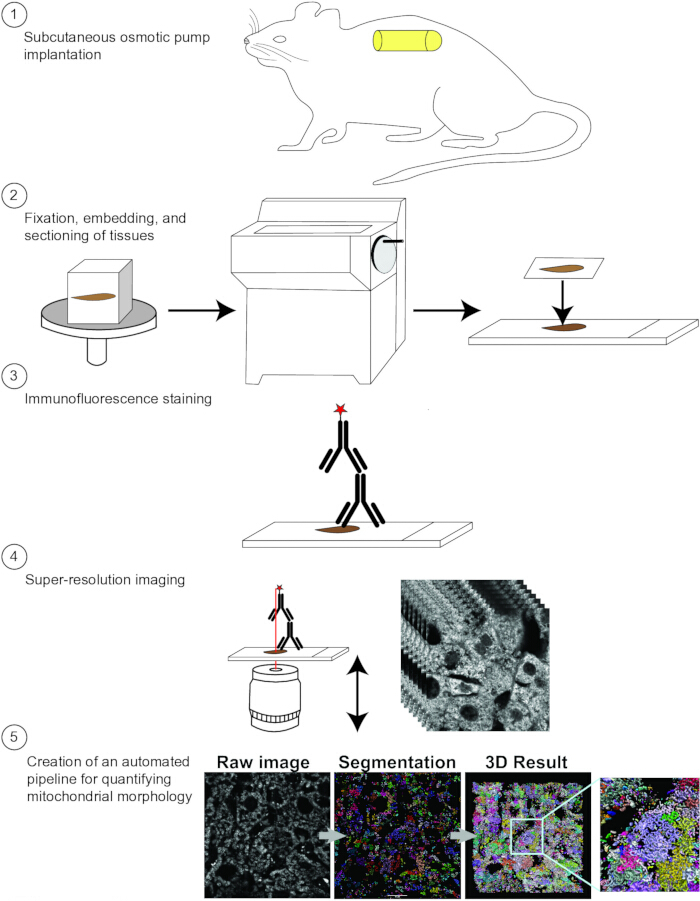
Figure 1: Overview of protocol. Mice are treated with drugs or a vehicle for up to 6 weeks using subcutaneous osmotic minipump implantation (1). Following treatment, the mouse tissues are fixed, infiltrated with sucrose, embedded in OCT Compound, and cryo-sectioned (2). The tissue sections are then stained with antibodies against Tom20 and secondary antibodies labeled with Alexa Fluor 568 (3). Super-resolution z-stacks are collected on an Airyscan2 point scanning confocal microscope (4), and the denoised processed z-stacks are segmented in arivis to quantify mitochondrial morphology (5). Please click here to view a larger version of this figure.

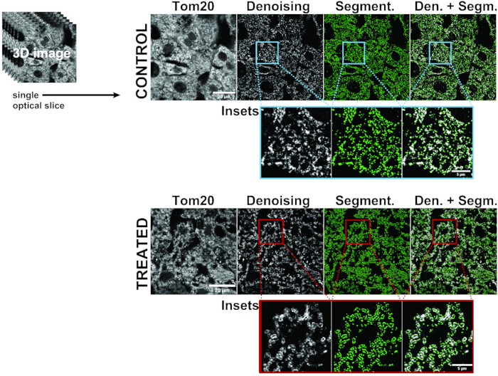
Figure 2: Automated pipeline for mitochondrial segmentation and morphology analysis.
Representative single optical slices from Control (upper panels) and Treated (lower panels) samples. The Tom20 immunofluorescence signal is shown in gray (left). The same image after denoising is displayed in gray, followed by the segmentation output highlighting detected mitochondrial objects in green. The merged image shows the overlap between the denoised signal and segmented objects. Insets show higher magnification views of the indicated regions, illustrating the effects of denoising and the accuracy of segmentation. Please click here to view a larger version of this figure.

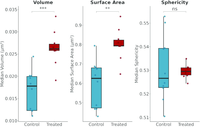
Figure 3: Mitochondrial morphology in the Control and Treated groups. Box plots show the median ± interquartile range of per-sample median values (n = 10 per group). Each dot represents one biological sample, summarized as the median across all mitochondria detected within that sample. Volume and surface area are displayed on a log₁₀ scale. Groups were compared using Wilcoxon rank-sum tests. Significance levels: ns p ≥ 0.05, **p < 0.01, ***p < 0.001. Please click here to view a larger version of this figure.

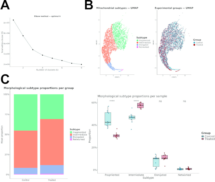
Figure 4: Unsupervised morphometric classification of mitochondrial subtypes. (A) Elbow plot showing the total within-cluster sum of squares (WSS) as a function of the number of clusters (k), calculated on a random subsample of 10,000 mitochondria. The inflection point at k = 4 was selected as the optimal number of clusters for downstream analysis. (B) (Left) UMAP dimensionality reduction of mitochondrial morphometric features (n = 20,000 randomly sampled mitochondria), colored by assigned subtype. Four morphologically distinct subtypes were identified: fragmented (small, high sphericity), elongated (long, low sphericity), networked (large, irregular), and intermediate. (Right) UMAP projection colored by experimental group (Control vs. Treated) showing the distribution of each group across the morphological space. (C) Per-sample proportions of each mitochondrial subtype in each experimental group. Each datapoint represents one biological sample (n = 10 per group). Box plots show the interquartile range and median, with whiskers extending to 1.5 times the interquartile range. Subtype proportions were compared between groups using the Wilcoxon rank-sum test, and p-values were corrected for multiple comparisons using the Benjamini-Hochberg method. ns p ≥ 0.05, ****p < 0.0001. Please click here to view a larger version of this figure.

Supplementary File 1: Example arivis pipeline. Please click here to download this file.

Supplementary File 2: R script for quantifying mitochondrial morphology and subtype populations.Please click here to download this file.

Discussion

The two most critical steps for successfully performing this protocol are (i) the closure of the incision during osmotic pump implantation, and (ii) accurate segmentation. For the former, take special care to create a subcutaneous pocket that is large enough for the pump, but not too large for the pump to slip down the flank of the animal. When the incision is closed, the pump should be placed sufficiently far away as not to induce any tension on the surrounding skin, which may lead to dehiscence. Make sure to tug on the skin surrounding the closed incision in all directions to verify that the wound is sufficiently closed before initiating animal recovery. Wound clips are advantageous as they are quick to apply and remove. However, if any issues arise from not being able to properly close the incisions, interrupted sutures may be used instead. For the latter, accurate segmentation requires you to constantly compare the segmentation results with the denoised images until there is sufficient image similarity. Z-stacks from Control and Treated animals must be collected using the same collection parameters and preferably during the same imaging session. Likewise, all processing steps must be applied to all images using the exact same parameters. The diameter segmentation parameter defines the expected size of the objects to be detected. A good starting point is the measured average mitochondrial width from a few manually inspected objects using one optical slice. The probability threshold controls the minimum detection confidence required for an object to be accepted. Lower values increase sensitivity and detect more objects, but some of these objects may be false. Conversely, higher values improve specificity but may cause objects with lower signal to be lost. A recommended starting range is 25%–30%. Finally, split sensitivity governs how aggressively touching or overlapping objects are separated into individual objects. A low split sensitivity will leave clustered mitochondria as single merged objects. On the other hand, a high split sensitivity can result in over-splitting of elongated or branched mitochondria into fragments. Values between 15%–30% are reasonable for typical mitochondrial morphological studies. If accurate segmentation still proves challenging, segmentation can be performed using Mitochondria Analyzer⁵⁹ in FIJI⁶⁰. A semi-automated pipeline for the quantification of mitochondrial morphologies in both cells and tissues using Huygens Professional software and a custom Python script has also been recently described⁶¹.

One limitation is the resolution limit of the Airyscan2 confocal microscope, which is ~150 nm in XY and ~350 nm in the Z-plane. This prevents high-resolution imaging of mitochondrial cristae, as distances between individual cristae are found to be ~40–120 nm^62,63,64. In contrast, stimulated emission depletion (STED) can reach resolution limits of ~20–50 nm laterally and can clearly distinguish individual mitochondrial cristae^62,63,64. Several STED dyes have recently been developed that allow for effective staining and imaging of the mitochondrial inner membrane in both live and fixed cells^63,64,65. Given that analysis of cristae morphologies may grant insights into mitochondrial bioenergetic health¹⁰, such data is therefore desired. However, mitochondrial morphology differs strongly between mammalian tissues and cell culture (discussed in-depth below), and there currently is no methodology to stain the inner membrane of tissues for STED imaging and analysis of cristae structures.

Quantifying mitochondrial morphology in intact tissue presents unique challenges compared to cell culture systems. In cultured cells, mitochondria are typically distributed throughout the cytoplasm in well-separated networks with minimal overlap between cells. In tissue sections or whole-mount preparations, however, cells are densely packed, and their boundaries are not well defined. If cell-level analysis is required, an additional fluorescent label targeting the plasma membrane or a cell-type-specific marker should be incorporated, along with a corresponding segmentation step in the image analysis pipeline to define individual cell boundaries before quantification of mitochondrial morphology. A second important difference is that in cultured cells, mitochondria often form continuous, interconnected reticular networks that are easy to visualize and interpret. In tissues, this pattern is rarely observed. For instance, mitochondria from liver sections demonstrate a punctate, rod and bundle pattern that occupies the entire cytosol⁶⁶. However, hepatocytes in culture show tubular morphologies with clear network formations⁶⁶. Similarly, when comparing mitochondria from smooth tissue with those from smooth muscle cells in culture, distinct differences are observed in their morphologies and network patterns⁶⁷. The three-dimensional architecture, combined with cell-type-specific differences in mitochondrial distribution, causes mitochondria in these tissues to appear as discrete, densely packed puncta or short fragments rather than elongated networks. Therefore, cautious interpretation of data is warranted when comparing morphological features between tissues and cell culture, as differences between the two may be partly attributable to imaging context rather than true biological variation.

A highlight of this protocol is the ability to quantitatively measure mitochondrial structures in tissues using light microscopy. While there exist other methods for quantifying mitochondrial morphology from super-resolution light microscopy images, many of them are suitable only for cells in culture. Moreover, in contrast to other analysis methods, the pipeline presented here is fully automated, quantifies both mitochondrial dimensions and subtype proportions, and requires little coding experience to successfully perform. Scanning/transmission electron microscopy (SEM/TEM) and cryo-ET have been previously used to image mitochondrial structures in tissues in 2D and 3D^10,68,69. However, for the former, there are concerns about the preservation of native structures following sample fixation, dehydration, and embedding^70,71. Moreover, manual measurement of mitochondrial parameters in FIJI⁶⁰ is sometimes the preferred analysis method for TEM images⁷², which requires significant work and may lead to sample bias. Deep-learning methods for automated quantification of mitochondrial morphologies from TEM images, however, have been recently described^73,74. An advantage of the presented approach is that once the analysis pipeline is established, it can batch-process images with little to no user input. For the latter, high-pressure freezing can preserve tissue structures in near-native conditions⁷⁵. However, cryo-ET sample freezing, sectioning, milling, data collection, and data processing all require extensive training and highly advanced equipment. In contrast, super-resolution confocal microscopy is relatively more accessible and requires less training and resources to successfully perform.

Osmotic pump implantations can safely be performed in aged mice to evaluate the effects of different pharmacological compounds on aging-related declines in physiological function. Additionally, the methods described herein are generalizable to many different organs. It is well-characterized that aging-related declines in metabolic function contribute to disease and arise from mitochondrial dysfunction, one of the colloquial hallmarks of aging⁷⁶. Furthermore, it is understood that mitochondrial structures inform mitochondrial bioenergetic capacity and metabolic status^77,78. Thus, quantitatively assessing compounds for their effects on mitochondrial structure during mouse aging, using the methods described herein, may aid in the identification of therapeutics that can prolong human healthspan.

Materials

List of materials used in this article

Name	Company	Catalog Number	Comments
Airyscan2 point scanning confocal microscope	ZEISS	LSM 980 with Airyscan2	ZEISS point scanning LSM 980 confocal built around a ZEISS Axio Observer Z1 and equipped with two multi-alkali PMTs and a GaASP 32 channel spectral detector, an environmental enclosure, and a Plan Apo 63×/1.4 Oil DIC III objective. The microscope used in this study is also equipped with two external NIR detectors, as well as the following laser lines: 405, 458, 488, 514, 561, 594, 639, and 730 nm.
Aluminum foil	Essendant	BWK7112
Analytical balance	Mettler Toledo	MR204
Anti-roll glass plate	Gel Company	LGI70
Arivis Pro Software	ZEISS	Version 4.1.2
Bath sonicator	Branson Ultrasonics	71020-MT
Bovine serum albumin	Research Products International	A30075
Centrifuge tubes, 15 mL	CELLTREAT	229411
Charged microscope slides	Globe Scientific	1358W
Clip remover	Alzet	0009976
CO2	Airgas	CD 50
Contrad 70	Decon Labs	1003
Cotton-tipped applicators	Puritan Medical	25-8061WC
Cryostat	Leica Biosystems	CM3050 S
Cryostat blades	Sakura Finetek USA Inc	4689
DAPI	Sigma-Aldrich	D9542	Prepare to 5 mg/mL in ddH2O, aliquot, and store at -20 °C protected from light
Dimethyl sulfoxide	Sigma-Aldrich	D2650
EasyDip slide staining system	Electron Microscopy Services	71388-01
Electro-Gel	Bio-Serv	EGS-1
Embedding molds, 22 mm ´ 22 mm ´ 20 mm	Polysciences	18646A-1
Ethanol, 200 proof	Decon Labs	V1001
Fenestrated sterile drape sheets	Dukal	20001
Fine forceps	Fine Science Tools	11445-12
Glass bead sterilizer	VWR	75999-324
Goat anti-rabbit Alexa Fluor 568	Invitrogen	A-11036
Heating pad	CVS	215313
Hemostatic forceps	World Precision Instruments	501705
Immersion oil Immersol 518 F	ZEISS	433802-9010-000
Induction chamber	World Precision Instruments	EZ178
Insulin syringes, 0.3 mL	BD	328431
Iris surgical scissors	Sklar Surgical Instruments	47-1135
Isoflurane	Patterson Veterinary	07-890-8115
Kimwipes	Kimberly-Clark	34120
Luer-Lok 1 mL syringes	BD	309628
Luer-Lok 3 mL syringes	BD	309657
Luer-Lok 50 mL syringes	BD	309653
Meloxivet (meloxicam)	Patterson Veterinary	07-894-8524
Microcentrifuge tubes, 1.5 mL	CELLTREAT	229443
Microscope slide box	Heathrow Scientific	15994E
Microscope slide cover glass, #1.5, 22 mm ´ 50 mm	Electron Microscopy Services	72204-04
Non-CO2 incubator	Benchmark Scientific	H2200-H
Non-fenestrated sterile drape sheets	Dukal	20-002
OCT Compound	Sakura Finetek USA Inc	4583
Opthalmic ointment	Patterson Veterinary	07-888-2572
Osmotic minipumps	Alzet	2004
Parafilm	Bemis	PM999
Paraformaldehyde, 4% w/v	Santa-Cruz Biotechnology	sc-281692
PBS, 1´	Thermo Scientific	10010023
PEG300	Sigma-Aldrich	90878
PES syringe filters, 0.22 µm	CELLTREAT	229747
Povidone iodine 10% USP swabsticks	Medline	MDS093901ZZ
ProLong Glass Antifade	Invitrogen	P36980
Rabbit anti-Tom20 antibody	Novus Biologicals	NBP2-67501
Razor blades, 0.22 mm	VWR	55411-050
Rotator/rotisserie	Labnet	H5500
RStudio	The R Project for Statistical Computing	version 4.3.2
Scale	Fisher Scientific	S72422
SomnoSuite low-flow anesthesia system	Kent Scientific	SS-01
Steam sterilization indicator strips	Crosstex	SIS-250
Sterile glass vials, 5 mL	Thermo Scientific	ST5
Sterile needles, 0.5", 23 G	BD	305145
Sterile needles, 0.5", 27 G	BD	305109
Sterilization pouches	Cardinal Health	92510
Sucrose	Sigma-Aldrich	S9378	Prepare a solution of 30% w/v in 1´ PBS
Surgical clippers	3M	9680
Surgical gloves	Cardinal Health	2D73DP75
Tissue forceps	Sklar Surgical Instruments	47-1447
Toploading balance	Cole-Parmer	EW-55000-14
Triton X-100	Sigma-Aldrich	T8787
Vetbond tissue adhesive	3M	1469SB
Weighing boats, 85 mL	Heathrow Scientific	1420B
Wound clip applier	Alzet	0009974
Wound clips, 7 mm	Alzet	0009971
Zen software	ZEISS	Zen Blue version 3.7.97.09000

References

- Iovine JC, Claypool SM, Alder NN. Mitochondrial compartmentalization: Emerging themes in structure and function. Trends Biochem Sci. 2021;46(11):902-917.
- Wolf DM, et al. Individual cristae within the same mitochondrion display different membrane potentials and are functionally independent. EMBO J. 2019;38(22):e101056.
- Jenkins BC, et al. Mitochondria in disease: Changes in shapes and dynamics. Trends Biochem Sci. 2024;49(4):346-360.
- Mesmin B. Mitochondrial lipid transport and biosynthesis: A complex balance. J Cell Biol. 2016;214(1):9-11.
- Fuhrmann DC, Brüne B. Mitochondrial composition and function under the control of hypoxia. Redox Biol. 2017;12:208-215.
- Strubbe-Rivera JO, et al. The mitochondrial permeability transition phenomenon elucidated by cryo-EM reveals the genuine impact of calcium overload on mitochondrial structure and function. Sci Rep. 2021;11(1):1037.
- Vercesi AE, et al. Mitochondrial calcium transport and the redox nature of the calcium-induced membrane permeability transition. Free Radic Biol Med. 2018;129:1-24.
- Chistiakov DA, et al. Mitochondrial aging and age-related dysfunction of mitochondria. Biomed Res Int. 2014;2014:238463.
- Daum B, Walter A, Horst A, Osiewacz HD, et al. Age-dependent dissociation of ATP synthase dimers and loss of inner-membrane cristae in mitochondria. Proc Natl Acad Sci U S A. 2013;110(38):15301-15306.
- Brandt T, et al. Changes of mitochondrial ultrastructure and function during ageing in mice and Drosophila. eLife. 2017;6:e24662.
- Liu YJ, McIntyre RL, Janssens GE, Houtkooper RH. Mitochondrial fission and fusion: A dynamic role in aging and potential target for age-related disease. Mech Ageing Dev. 2020;186:111212.
- Zhang X, et al. Mitochondrial dysfunction in the regulation of aging and aging-related diseases. Cell Commun Signal. 2025;23(1):290.
- Rottenberg H, Hoek JB. The mitochondrial permeability transition: Nexus of aging, disease and longevity. Cells. 2021;10(1):79.
- Ekblom-Bak E, et al. Sex- and age-specific associations between cardiorespiratory fitness, cardiovascular disease morbidity and all-cause mortality in 266,109 adults. Prev Med. 2019;127:105799.
- Harber MP, et al. Impact of cardiorespiratory fitness on all-cause and disease-specific mortality: Advances since 2009. Prog Cardiovasc Dis. 2017;60(1):11-20.
- Goulding RP, et al. Skeletal muscle mitochondrial fragmentation predicts age-associated decline in physical capacity. Aging Cell. 2025;24(2):e14386.
- Amorim JA, et al. Mitochondrial and metabolic dysfunction in ageing and age-related diseases. Nat Rev Endocrinol. 2022;18(4):243-258.
- Srivastava S. The mitochondrial basis of aging and age-related disorders. Genes (Basel). 2017;8(12):398.
- Toescu EC, Myronova N, Verkhratsky A. Age-related structural and functional changes of brain mitochondria. Cell Calcium. 2000;28(5-6):329-338.
- Reed AL, Mitchell W, Alexandrescu AT, Alder NN. Interactions of amyloidogenic proteins with mitochondrial protein import machinery in aging-related neurodegenerative diseases. Front Physiol. 2023;14:1263420.
- Reeve AK, et al. Mitochondrial dysfunction within the synapses of substantia nigra neurons in Parkinson's disease. NPJ Parkinsons Dis. 2018;4:9.
- Chen C, et al. Astrocytic changes in mitochondrial oxidative phosphorylation protein levels in Parkinson's disease. Mov Disord. 2022;37(2):302-314.
- Patyal P, et al. Mitochondrial dynamics in aging heart. Biomedicines. 2025;13(11):2603.
- Hinton A, et al. Mitochondrial structure and function in human heart failure. Circ Res. 2024;135(2):372-396.
- Bernardi P, et al. Identity, structure, and function of the mitochondrial permeability transition pore: Controversies, consensus, recent advances, and future directions. Cell Death Differ. 2023;30(8):1869-1885.
- Wang D, Ji DC, Yu CY, Wu DN, Qi L. Research progress on the mitochondrial mechanism of age-related non-alcoholic fatty liver. World J Gastroenterol. 2023;29(13):1982-1993.
- Lionetti L, et al. High-lard and high-fish-oil diets differ in their effects on function and dynamic behaviour of rat hepatic mitochondria. PLoS One. 2014;9(3):e92753.
- Mitchell W, et al. The mitochondria-targeted peptide SS-31 binds lipid bilayers and modulates surface electrostatics as a key component of its mechanism of action. J Biol Chem. 2020;295(21):7452-7469.
- Roshanravan B, et al. In vivo mitochondrial ATP production is improved in older adult skeletal muscle after a single dose of elamipretide in a randomized trial. PLoS One. 2021;16(7):e0253849.
- Sabbah HN, et al. Chronic therapy with elamipretide (MTP-131), a novel mitochondria-targeting peptide, improves left ventricular and mitochondrial function in dogs with advanced heart failure. Circ Heart Fail. 2016;9(2):e002206.
- Finsterer J. Barth syndrome: Mechanisms and management. Appl Clin Genet. 2019;12:95-106.
- Mitchell W, et al. The mitochondria-targeted peptide therapeutic elamipretide improves cardiac and skeletal muscle function during aging without detectable changes in tissue epigenetic or transcriptomic age. Aging Cell. 2025;24(6):e70026.
- Pharaoh G, et al. The mitochondrially targeted peptide elamipretide (SS-31) improves ADP sensitivity in aged mitochondria by increasing uptake through the adenine nucleotide translocator (ANT). GeroScience. 2023;45(6):3529-3548.
- Campbell MD, et al. Improving mitochondrial function with SS-31 reverses age-related redox stress and improves exercise tolerance in aged mice. Free Radic Biol Med. 2019;134:268-281.
- Campbell MD, et al. Intermittent treatment with elamipretide preserves exercise tolerance in aged female mice. GeroScience. 2023;45(4):2245-2255.
- Ryu D, et al. Urolithin A induces mitophagy and prolongs lifespan in C. elegans and increases muscle function in rodents. Nat Med. 2016;22(8):879-888.
- Liu S, et al. Effect of urolithin A supplementation on muscle endurance and mitochondrial health in older adults: A randomized clinical trial. JAMA Netw Open. 2022;5(1):e2144279.
- Singh A, et al. Urolithin A improves muscle strength, exercise performance, and biomarkers of mitochondrial health in a randomized trial in middle-aged adults. Cell Rep Med. 2022;3(5):100633.
- Liu S, et al. Urolithin A provides cardioprotection and mitochondrial quality enhancement preclinically and improves human cardiovascular health biomarkers. iScience. 2025;28(2):111814.
- Fontaine E. Metformin-induced mitochondrial complex I inhibition: Facts, uncertainties, and consequences. Front Endocrinol (Lausanne). 2018;9:753.
- Martin-Montalvo A, et al. Metformin improves healthspan and lifespan in mice. Nat Commun. 2013;4(1):2192.
- Lee SH, Min KJ. Caloric restriction and its mimetics. BMB Rep. 2013;46(4):181-187.
- Pal RS, et al. Metformin's anticancer odyssey: Revealing multifaceted mechanisms across diverse neoplastic terrains—a critical review. Biochimie. 2025;233:109-121.
- Zhang JH, et al. Metformin use is associated with a reduced risk of cognitive impairment in adults with diabetes mellitus: A systematic review and meta-analysis. Front Neurosci. 2022;16:984559.
- Keys MT, Hallas J, Miller RA, Suissa S, Christensen K. Emerging uncertainty on the anti-aging potential of metformin. Ageing Res Rev. 2025;111:102817.
- Khan NA, et al. Effective treatment of mitochondrial myopathy by nicotinamide riboside, a vitamin B3. EMBO Mol Med. 2014;6(6):721-731.
- Cantó C, et al. The NAD+ precursor nicotinamide riboside enhances oxidative metabolism and protects against high-fat diet-induced obesity. Cell Metab. 2012;15(6):838-847.
- Lapatto HAK, et al. Nicotinamide riboside improves muscle mitochondrial biogenesis, satellite cell differentiation, and gut microbiota in a twin study. Sci Adv. 2023;9(2):eadd5163.
- Zhou Q, et al. Nicotinamide riboside enhances mitochondrial proteostasis and adult neurogenesis through activation of mitochondrial unfolded protein response signaling in the brain of ALS SOD1(G93A) mice. Int J Biol Sci. 2020;16(2):284-297.
- Harrison DE, et al. 17-α-Estradiol late in life extends lifespan in aging UM-HET3 male mice; nicotinamide riboside and three other drugs do not affect lifespan in either sex. Aging Cell. 2021;20(5):e13328.
- Wu J, et al. Transcardiac perfusion of the mouse for brain tissue dissection and fixation. Bio Protoc. 2021;11(5):e3988.
- Wehrl HF, et al. Assessment of murine brain tissue shrinkage caused by different histological fixatives using magnetic resonance and computed tomography imaging. Histol Histopathol. 2015;30(5):601-613.
- Mitchell W, et al. In vivo chemical reprogramming is associated with a toxic accumulation of lipid droplets hindering rejuvenation. Aging Cell. 2026;25(2):e70390.
- Liaw A, Wiener MC. Classification and regression by randomForest. R News. 2002;2(3):18-22.
- Kuhn M. Building predictive models in R using the caret package. J Stat Softw. 2008;28(5):1-26.
- Thorndike RL. Who belongs in the family? Psychometrika. 1953;18(4):267-276.
- MacQueen J. Some methods for classification and analysis of multivariate observations. Proceedings of the 5th Berkeley Symposium on Mathematical Statistics and Probability Oakland, CA, USA. 1967:281-297.
- Hartigan JA, Wong MA. Algorithm AS 136: A K-means clustering algorithm. J R Stat Soc Ser C Appl Stat. 1979;28(1):100-108.
- Chaudhry A, Shi R, Luciani DS. A pipeline for multidimensional confocal analysis of mitochondrial morphology, function, and dynamics in pancreatic β-cells. Am J Physiol Endocrinol Metab. 2020;318(2):E87-E101.
- Schindelin J, et al. Fiji: An open-source platform for biological-image analysis. Nat Methods. 2012;9(7):676-682.
- Negri E, Fernández V, Borrell V. MitoLandscape, a semi-automated pipeline for subcellular localization and quantification of mitochondria. Front Cell Dev Biol. 2025;13:1668779.
- Ng EL, Reed AL, O'Connell CB, Alder NN. Using live-cell STED imaging to visualize mitochondrial inner membrane ultrastructure in neuronal cell models. J Vis Exp. 2023;196:e65561.
- Yang X, et al. Mitochondrial dynamics quantitatively revealed by STED nanoscopy with an enhanced squaraine variant probe. Nat Commun. 2020;11(1):3699.
- Liu T, et al. Multi-color live-cell STED nanoscopy of mitochondria with a gentle inner membrane stain. Proc Natl Acad Sci U S A. 2022;119(52):e2215799119.
- Chen J, et al. An aldehyde-crosslinking mitochondrial probe for STED imaging in fixed cells. Proc Natl Acad Sci U S A. 2024;121(19):e2317703121.
- Das S, et al. Mitochondrial morphology and dynamics in hepatocytes from normal and ethanol-fed rats. Pflugers Arch. 2012;464(1):101-109.
- McCarron JG, et al. From structure to function: Mitochondrial morphology, motion and shaping in vascular smooth muscle. J Vasc Res. 2013;50(5):357-371.
- Lea PJ, Hollenberg MJ. Mitochondrial structure revealed by high-resolution scanning electron microscopy. Am J Anat. 1989;184(3):245-257.
- McMillan JD, Eisenback MA. Transmission electron microscopy for analysis of mitochondria in mouse skeletal muscle. Bio Protoc. 2018;8(10):e2455.
- Teixeira P, Galland R, Chevrollier A. Super-resolution microscopies: Technological breakthrough to decipher mitochondrial structure and dynamic. Semin Cell Dev Biol. 2024;159-160:38-51.
- Neikirk K, et al. Systematic transmission electron microscopy-based identification and 3D reconstruction of cellular degradation machinery. Adv Biol (Weinh). 2023;7(6):2200221.
- Lam J, et al. A universal approach to analyzing transmission electron microscopy with ImageJ. Cells. 2021;10(9):2177.
- Jang C, Lee H, Yoo J, Yoon H. Deep learning-driven automated mitochondrial segmentation for analysis of complex transmission electron microscopy images. Sci Rep. 2025;15(1):19076.
- Conrad R, Narayan K. Instance segmentation of mitochondria in electron microscopy images with a generalist deep learning model trained on a diverse dataset. Cell Syst. 2023;14(1):58-71.e5.
- Garcia GC, et al. Mitochondrial morphology provides a mechanism for energy buffering at synapses. Sci Rep. 2019;9(1):18306.
- López-Otín C, Blasco MA, Partridge L, Serrano M, et al. Hallmarks of aging: An expanding universe. Cell. 2023;186(2):243-278.
- Mannella CA, Lederer WJ, Jafri MS. The connection between inner membrane topology and mitochondrial function. J Mol Cell Cardiol. 2013;62:51-57.
- Glancy B, Kim Y, Katti P, Willingham TB. The functional impact of mitochondrial structure across subcellular scales. Front Physiol. 2020;11:541040.
Reprints and Permissions
This article has been published
Video Coming Soon