This protocol describes a network pharmacology and molecular docking workflow for identifying potential targets, signaling pathways, and compound–target interactions of Sishen Decoction in gout.
A subscription to JoVE is required to view this content. Sign in or start your free trial.
Research Article
Integrated Network Pharmacology and Molecular Docking Analysis of Sishen Decoction Identifies Potential Targets and Pathways in Gout
In This Article
Summary
Abstract
Gout is a disease characterized by hyperuricemia and the deposition of urate crystals in joints and soft tissues, leading to recurrent acute arthritis. Its increasing prevalence imposes substantial clinical and socioeconomic burdens. Sishen Decoction (SSD) has been used in the treatment of gout, but its potential molecular mechanisms remain unclear. This study applied an integrated network pharmacology and molecular docking approach to identify potential targets and signaling pathways associated with SSD in gout. Active compounds and corresponding targets of SSD were retrieved from the Traditional Chinese Medicine Systems Pharmacology Database (TCMSP), while gout-related targets were collected from the GeneCards and Online Mendelian Inheritance in Man (OMIM) databases. Overlapping targets were identified and used to construct a drug–component–target–disease network. A protein–protein interaction (PPI) network was established using the Search Tool for the Retrieval of Interacting Genes/Proteins (STRING) database. Gene Ontology (GO) and Kyoto Encyclopedia of Genes and Genomes (KEGG) enrichment analyses were performed, followed by molecular docking using the docking server analysis module. A total of 37 bioactive compounds were associated with 116 overlapping gout-related targets. The top hub targets included TP53, IL6, IL1B, TNF, AKT1, EGFR, CASP3, JUN, BCL2, and MMP9. GO analysis suggested that these targets are involved in gene expression regulation and signal transduction. KEGG enrichment analysis indicated significant associations with the mitogen-activated protein kinase (MAPK), phosphoinositide 3-kinase/protein kinase B (PI3K-Akt), interleukin-17 (IL-17), and tumor necrosis factor (TNF) signaling pathways. Molecular docking predicted favorable interactions between key compounds and hub targets, with all binding energies of ≤−5 kcal/mol. These computational findings provide potential mechanistic hypotheses for the action of SSD in gout and may support future experimental validation.
Introduction
Gout is a disease characterized by hyperuricemia and the deposition of urate crystals in joints and soft tissues, leading to recurrent acute arthritis1. Its hallmark features include recurrent episodes of severe pain, redness, swelling, and impaired joint function2,3. Driven by major dietary risk factors such as high-purine and high-sugar intake, as well as excessive alcohol consumption, the prevalence of gout has risen significantly, making it a serious public health issue that not only impairs patients’ quality of life but also imposes substantial socioeconomic burdens4,5,6. Effective gout treatment aims to both resolve acute inflammatory flares and achieve long-term reduction of serum uric acid levels7,8. The use of nonsteroidal anti-inflammatory drugs, colchicine, or glucocorticoids to control acute gout inflammation is frequently accompanied by a range of adverse effects, most commonly gastrointestinal disturbances9,10. In addition, urate-lowering drugs such as benzbromarone, allopurinol, and febuxostat carry risks of hepatotoxicity and hypersensitivity, which restrict their broader clinical use11,12. Therefore, exploring novel therapeutic strategies that are safe, effective, and supported by clearly defined mechanisms remains of considerable clinical importance.
The clinical practice of Traditional Chinese Medicine (TCM) in the prevention and treatment of gout has a long history. Practitioners across successive dynasties have accumulated extensive experience in applying TCM to manage this condition, with well-documented therapeutic efficacy. Through holistic regulation and multi-pathway intervention of pathological processes, TCM demonstrates distinctive therapeutic advantages13. Sishen Decoction (SSD), derived from the Qing dynasty text Newly Compiled Proven Formulas, consists of five medicinal herbs: Astragalus membranaceus (Huangqi), Polygala tenuifolia (Yuanzhi), Achyranthes bidentata (Huainiuxi), Dendrobium nobile (Shihu), and Lonicera japonica (Jinyinhua). SSD has been reported to reduce uric acid levels and improve the quality of life of patients with gout by reinforcing vital qi, dispelling pathogenic factors, and unblocking collaterals to relieve pain14,15. These therapeutic effects are consistent with the holistic regulatory principles of TCM. Its potential activity may involve modulation of the complex immune–metabolic–neuroendocrine network, thereby influencing the pathological environment associated with gout16. However, the molecular basis underlying the therapeutic effects of SSD in gout remains unclear. Furthermore, despite previous investigations of SSD in other inflammatory disorders, its potential targets and pathways in gout have not been systematically explored using an integrated computational approach.
Network pharmacology, an emerging discipline that integrates systems biology and polypharmacology, adopts a holistic “disease–gene–target–drug” strategy that aligns naturally with the multicomponent and multi-target characteristics of TCM formulas17,18. Molecular docking complements this approach by predicting the binding modes and affinities between active compounds and target proteins at the molecular level, thereby providing supportive evidence for predicted interactions19. The combination of network pharmacology-based global screening and molecular docking-based target assessment can improve the reliability of target prediction and reduce the likelihood of false-positive findings associated with a single analytical method20. Importantly, the results generated by these computational approaches provide testable hypotheses that require subsequent experimental validation. Given that the molecular mechanisms of SSD in gout remain poorly understood, the present study employed an integrated network pharmacology and molecular docking strategy to identify potential targets, signaling pathways, and compound–target interactions associated with SSD in gout.
Access restricted. Please log in or start a trial to view this content.
Protocol
This database-based computational study does not involve human participants, animal experiments, or clinical samples. According to Article 32 of China’s Measures for Ethical Review of Life Sciences and Medical Research Involving Human Subjects, studies that use lawfully obtained publicly available data, do not cause harm to human subjects, involve no sensitive personal information, and have no commercial interests are eligible for exemption from ethical review. Therefore, ethical approval is not required for this study.
The experimental design and analytical pipeline of this study are illustrated in the flowchart (Figure 1).
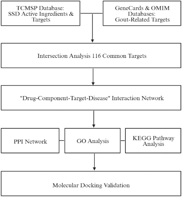
Figure 1: Overall Workflow of the Study. The flowchart illustrates the sequential workflow of the network pharmacology and molecular docking analyses, including the acquisition of active components and targets of Sishen Decoction (SSD), collection of gout-related targets, identification of overlapping targets, construction of the drug–component–target–disease network and protein–protein interaction (PPI) network, Gene Ontology (GO) and Kyoto Encyclopedia of Genes and Genomes (KEGG) enrichment analyses, and molecular docking simulations. Please click here to view a larger version of this figure.
Acquisition of Active Components and Target Proteins of SSD
On January 2, 2026, the active chemical components of the five herbs constituting SSD, namely Huangqi, Yuanzhi, Huainiuxi, Shihu, and Jinyinhua, were retrieved from the Traditional Chinese Medicine Systems Pharmacology (TCMSP) database21. Screening criteria based on pharmacokinetic properties were applied: oral bioavailability (OB) of ≥30% and drug-likeness (DL) of ≥0.1822. Components meeting these criteria were considered potential active ingredients. Corresponding targets for each component were then collected. Since TCMSP lacked complete data for Yuanzhi and Shihu, the chemical components of these two herbs were additionally retrieved from the Herb 2.0 database on the same day. After obtaining the component names, a reverse search was performed in TCMSP using the component names and corresponding CAS numbers as keywords to retrieve target information. For compounds obtained from the Herb database, only those successfully matched to entries in TCMSP by either component name or CAS number were retained. The matched compounds were then subjected to the same pharmacokinetic screening criteria (OB ≥ 30% and DL ≥ 0.18) using TCMSP data, and compounds lacking complete OB or DL information were excluded. All matched and filtered compounds were manually verified against the original Herb 2.0 records to prevent misidentification. Subsequently, the target information derived from the Herb database was merged with that of the remaining herbs to generate the complete set of active ingredient targets for SSD.
All retrieved target proteins were standardized to official gene symbols using the UniProt database. A one-to-one correspondence was established by retaining only human-reviewed (Swiss-Prot) entries and excluding unreviewed (TrEMBL) entries. When multiple isoforms corresponded to the same gene symbol, the canonical isoform was selected. The standardized target dataset was retained for subsequent intersecting gene analysis.
Collection of Gout-Related Targets
On January 2, 2026, systematic searches were conducted in the GeneCards database and the OMIM database using “gout” as the disease keyword to obtain gout-related disease targets. The targets obtained from the two databases were exported to WPS Spreadsheets (version 12.1.0). The Gene Symbol column from OMIM was positioned adjacent to the Gene Symbol column from GeneCards, and duplicate targets were removed using the “Remove Duplicates” function based on exact matches of official gene symbols in a case-insensitive manner. The targets from the two databases were then merged to construct a comprehensive set of gout-related disease targets.
Identification of Drug–Disease Overlapping Targets
The drug target set obtained from active component screening and the gout-related disease target set were placed in the same project folder (D:\Venn). R software (version 4.4.0) was launched, and the readxl package was used to import Excel (.xlsx) files containing the target lists. The dplyr package was used for data manipulation, including filtering and renaming columns prior to intersection analysis. The two target sets were then converted into character vectors, and overlapping targets were identified using the calculate.overlap() function from the VennDiagram package. The VennDiagram package was installed from CRAN using the command install.packages(“VennDiagram”) and stored in the default R library path. If a message indicating that the package had already been installed appeared, the installation was considered successful. The working directory was set using the command setwd(“D:\\Venn”), which designated the folder containing the input files and served as the output directory. The R script was then executed to calculate the intersection between the drug target set and the gout-related disease target set. The resulting overlapping targets were defined as potential therapeutic targets of SSD for the treatment of gout.
Construction of the “Drug-Component-Target-Disease” Network
The intersecting genes identified from the overlap between SSD targets and gout-related targets were saved as the overlapping_targets.txt file, and the active component information of SSD was saved as the drug_components.txt file. Both files were placed in the project folder (D:\Network), which served as the working directory for the analysis. To ensure reproducibility, this analysis was performed using R. Data reading, filtering, and merging operations were carried out using a combination of base R functions, including read.table(), write.table(), and merge(), together with the dplyr package for data-frame manipulation. The command setwd("D:\Network") was executed to explicitly define the working directory.
The graph_from_data_frame() function was used as the core integration function. Each row of drug_components.txt linked an active component to its corresponding target gene using official gene symbols. Only targets present in overlapping_targets.txt were retained, and no additional filtering was applied beyond the intersection requirement. The resulting network dataset was exported as network.txt in edge-list format. Each row contained two columns (node1 and node2), where node1 represented either the SSD formula or an active component, and node2 represented either an active component or a target gene. The disease node (“gout”) was connected to the SSD formula as a separate edge. Edge weights were not assigned, and all edges were treated equally (edge width = 0.8).
The network.txt file was imported into the Cytoscape (version 3.7.2) network visualization software. The built-in NetworkAnalyzer tool was accessed through Tools → Network Analysis → Analyze Network to obtain the basic network structure, and “Degree Distribution” was selected as the analytical framework. Node shapes and colors were assigned according to node types: blue diamonds represented the SSD formula, blue rectangles represented active components, orange ellipses represented disease target genes, and red octagons represented the gout disease entity. Node size was set to be proportional to node degree (node size = 30 + degree × 5, maximum size = 100).
Construction of the Protein–Protein Interaction (PPI) Network
The filtered set of intersecting target genes was imported into the STRING database (version 12.0) on January 2, 2026. The species was restricted to Homo sapiens, the minimum interaction confidence threshold was set to high confidence (0.700), disconnected proteins were hidden, interaction sources included all available evidence channels, and all other parameters were maintained at their default settings to obtain known and predicted protein–protein interactions. The resulting network data were exported in tab-separated values (TSV) format using the default export options.
The exported network was imported into the network visualization software for visualization and topological analysis. Network properties were calculated using the built-in NetworkAnalyzer tool (Tools → Network Analysis → Analyze Network). The calculated metrics included degree, betweenness centrality, and closeness centrality. Node sizes were mapped to degree values using a continuous mapping function (node size = 20 + degree × 3, maximum size = 80).
Hub targets were identified by ranking all nodes according to degree values in descending order. Nodes with higher degree values were considered more central within the network. Isolated nodes (degree = 0) were excluded from visualization. The network layout was arranged in concentric circles from the center outward according to node connectivity, and node colors were mapped using a blue-to-cyan gradient corresponding to increasing degree values. The resulting network was used to identify the core hub targets involved in the potential therapeutic effects of SSD against gout.
Gene Ontology (GO) Enrichment Analysis
Based on the identified overlapping target genes, GO functional enrichment analysis was performed using R. Required Bioconductor packages were installed in the default R library path and loaded into the analysis environment. The intersecting gene file was stored in the project directory (D:\GO), and the working directory was defined using the setwd() function.
Gene identifier conversion and annotation were performed using the Bioconductor package org.Hs.eg.db (version 3.20.0). Official gene symbols were converted to Entrez Gene IDs using the bitr() function in the clusterProfiler enrichment analysis package (version 4.21.0). Only genes showing unique one-to-one mappings were retained for downstream analyses, whereas ambiguous or unmapped entries were excluded.
GO enrichment analysis was conducted using the enrichment analysis package. The enrichGO() function was used with the ontology categories Biological Process (BP), Cellular Component (CC), and Molecular Function (MF). Statistical significance was determined using the Benjamini–Hochberg multiple-testing correction method, with an adjusted P-value < 0.05 considered significant.
For each ontology category, significantly enriched terms were ranked according to the enrichment factor:
EF = (gene count / total background genes) ÷ (term size / total genome genes)
The top 10 terms were selected for detailed analysis. When identical enrichment factors occurred, terms with lower adjusted P-values were ranked higher.
Enrichment results were visualized using ggplot2 (version 3.5.1) and enrichplot (version 1.24.0). Bubble plots and bar charts were generated using the dotplot() and barplot() functions. Bubble size represented the number of enriched genes, whereas color corresponded to enrichment significance expressed as −log10(adjusted P-value). Default plotting parameters were used throughout.
KEGG Pathway Enrichment Analysis
KEGG pathway enrichment analysis of the intersecting targets of SSD and gout was performed using R and the previously described enrichment analysis package. Gene symbols were converted into KEGG-compatible identifiers using the bitr() function provided by the enrichment analysis package, with KEGG serving as the annotation resource. Pathway enrichment analysis was conducted using the enrichKEGG() function based on the hypergeometric test. Statistical significance was determined using the Benjamini–Hochberg (BH) multiple-testing correction method, and pathways with an adjusted P-value < 0.05 were considered significantly enriched.
Enrichment results were exported to Microsoft Excel-compatible workbook files using the openxlsx package (version 4.2.8.1) and the write.xlsx() function for subsequent review and figure preparation.
A multilevel target–pathway interaction network was subsequently constructed using the network visualization software. Network data were imported using File → Import → Network from File. Nodes consisted of target gene nodes and significantly enriched KEGG pathway nodes (BH-adjusted P-value < 0.05), whereas edges represented documented associations between target genes and enriched pathways identified during enrichment analysis. Network visualization was performed using the Style panel of the network visualization software, with target genes displayed as grey ellipses and pathways displayed as cyan rectangles. No additional plugins were used. The network was manually generated from the enrichment output table to visualize the relationships between core targets and significantly enriched pathways.
Molecular Docking Validation
The 3D structure files (MOL2 format) of the top 10 active components ranked by target connectivity in the “drug–component–target–disease” network were downloaded from the TCMSP database. Target connectivity was defined as the node degree (i.e., the number of direct connections between an active component and target genes in the network). Active components were ranked in descending order according to degree values, and the top 10 components were selected for molecular docking analysis.
The crystal structures of the top 10 hub target proteins identified from the PPI network were obtained from the RCSB Protein Data Bank (PDB) on January 23, 2026. The species was restricted to Homo sapiens. For each target protein, the structure with the highest crystallographic resolution (lowest Å value), without mutations, and co-crystallized with a native ligand or inhibitor was preferentially selected. If multiple structures met these criteria, the structure with the highest resolution and most complete protein sequence coverage was selected. The following PDB structures were used: 1GKC (MMP9), 5WHH (BCL2), 2P33 (JUN), 1RHJ (CASP3), 1WT5 (EGFR), 7APJ (AKT1), 1DU3 (TNF), 1T4Q (IL1B), 4NI9 (IL6), and 9CKJ (TP53).
Molecular docking simulations were performed using the CB-Dock 2 online server (web version, accessed January 23, 2026), which employs AutoDock Vina as the docking engine. Protein structures were automatically preprocessed by the server, including removal of heteroatoms and preparation of receptor structures. Ligands were uploaded in MOL2 format. Template-independent cavity detection was used, with five potential binding cavities automatically identified for each protein structure. Docking calculations were performed using the docking engine default parameters: exhaustiveness = 8, energy range = 4, and maximum number of binding modes = 9.
For each target–compound pair, docking was performed independently within each of the five detected cavities. Docking poses were evaluated using the docking engine scoring function, and the pose with the lowest binding energy within each cavity was retained as the representative conformation for that cavity. Among the five representative conformations, the docking pose with the globally lowest binding energy was selected as the final docking result for that target–compound pair and used for subsequent analyses.
The lowest binding energy value obtained for each docking result was recorded in a spreadsheet and imported into the Weishengxin online plotting platform (accessed January 23, 2026) to generate a heatmap using default parameters. The heatmap employed a yellow-to-red color gradient, complete-linkage hierarchical clustering, and Euclidean distance as the clustering metric.
Hydrogen-bond interactions were automatically identified by the docking server analysis module based on geometric criteria. A hydrogen bond was defined as an interaction with a donor–acceptor distance ≤ 3.5 Å and a donor–hydrogen–acceptor angle ≥ 120°. Hydrogen bonds were displayed as dashed lines in both two-dimensional and three-dimensional interaction diagrams. The target protein–active component pair exhibiting the globally lowest binding energy among all docking combinations was selected for detailed interaction analysis. This selection was based on a single target–compound pair rather than an individual docking pose and was intended to identify the strongest predicted interaction within the network. The final representative docking pose corresponding to this target–compound pair was used for visualization and interaction analysis.
Three-dimensional and two-dimensional interaction diagrams were generated using ChimeraX version 1.5 and LigPlot+ version 2.2, respectively. In ChimeraX, proteins were displayed using the default cartoon representation, ligands were displayed in stick mode, hydrogen bonds were shown as dashed lines, and the default color scheme was applied. In LigPlot+, hydrogen-bond identification was performed using the HBPLUS algorithm with a donor–acceptor distance threshold of 3.9 Å and an angle threshold of 90°. All other visualization parameters were retained at their default settings.
Access restricted. Please log in or start a trial to view this content.
Results
Therapeutic Targets of SSD for Gout
A total of 62 active components of SSD meeting the screening criteria were retrieved from the TCMSP database, corresponding to 3,634 targets. Gout-related targets were obtained from GeneCards and OMIM, and after duplicate removal, a total of 3,691 targets were collected. The intersection between the targets associated with SSD active components and the gout-related disease targets yielded 116 common targets, which were considered potential therapeutic targets of SS...
Access restricted. Please log in or start a trial to view this content.
Discussion
Gouty arthritis is a crystal arthropathy caused by the deposition of urate crystals in the joints as a consequence of hyperuricemia. Monosodium urate (MSU) crystals within the joint cavity are recognized by pattern recognition receptors on the surface of macrophages and neutrophils, leading to activation of the NOD-like receptor family pyrin domain-containing 3 (NLRP3) inflammasome and subsequent release of IL-1β23. This process further triggers signaling pathways, including the MAPK, NF-_...
Access restricted. Please log in or start a trial to view this content.
Disclosures
The authors declare no conflicts of interest.
Acknowledgements
The authors declare that no financial support was received for this work or its publication.
Access restricted. Please log in or start a trial to view this content.
Materials
| Name | Company | Catalog Number | Comments |
|---|---|---|---|
| AutoDock Vina | The Scripps Research Institute | Version integrated within the CB-Dock 2 web server | Docking engine used for molecular docking calculations and binding energy scoring |
| CB-Dock 2 | Liu et al. (Nucleic Acids Research, 2022) | Web version (released May 2022); accessed on January 23, 2026; URL: https://cadd.labshare.cn/cb-dock2 | Used for molecular docking simulations between active compounds and target proteins |
| ChimeraX | UCSF Resource for Biocomputing, Visualization, and Informatics | Version 1.5 | Used for three-dimensional visualization of docking complexes |
| clusterProfiler | Bioconductor | Version 4.21.0 | Used for GO and KEGG enrichment analyses |
| Cytoscape | Cytoscape Consortium / Institute for Systems Biology | Version 3.7.2 | Used for network construction, visualization, and PPI analysis |
| dplyr | CRAN | Version 1.2.1 | Used for data manipulation and network dataset generation |
| enrichplot | Bioconductor | Version 1.24.0 | Used for visualization of GO and KEGG enrichment results |
| GeneCards | Crown Human Genome Center, Weizmann Institute of Science | Version 5.26; accessed on January 2, 2026; URL: https://www.genecards.org | Used for retrieval of gout-related disease targets |
| ggplot2 | CRAN | Version 3.5.1 | Used for visualization of GO enrichment results |
| Herb Database | Fang et al. (Nucleic Acids Research, 2024) | Version 2.0 (released March 15, 2023); accessed on January 2, 2026; URL: http://herb.ac.cn/v2 | Used for supplementing active compound information for Yuanzhi and Shihu |
| LigPlot+ | European Bioinformatics Institute (EMBL-EBI) | Version 2.2 | Used for generating two-dimensional protein–ligand interaction diagrams |
| OMIM (Online Mendelian Inheritance in Man) | McKusick-Nathans Institute of Genetic Medicine, Johns Hopkins University School of Medicine | Accessed on January 2, 2026; URL: https://omim.org | Used for retrieval of gout-related disease targets |
| openxlsx | CRAN | Version 4.2.8.1 | Used for spreadsheet export and processing |
| org.Hs.eg.db | Bioconductor | Version 3.20.0 | Human genome annotation package used for gene identifier conversion and annotation |
| Protein Data Bank (RCSB PDB) | RCSB PDB | Accessed on January 23, 2026; URL: https://www.rcsb.org | Used for obtaining protein crystal structures |
| R (The R Project for Statistical Computing) | R Foundation for Statistical Computing | Version 4.4.0 | Used for data processing, enrichment analysis, and network generation |
| readxl | CRAN | Version 1.5.0 | Used for spreadsheet import and data processing |
| STRING Database | EMBL / Szklarczyk et al. | Version 12.0 (accessed on January 2, 2026); URL: https://string-db.org | Used for construction of the PPI network |
| Traditional Chinese Medicine Systems Pharmacology Database and Analysis Platform (TCMSP) | Center for Bioinformatics, Northwest A&F University / Dalian University of Technology | Version 2.3 (accessed on January 2, 2026); URL: https://tcmsp-e.com | Used for retrieval of active compounds and corresponding targets |
| UniProt (Universal Protein Resource) | UniProt Consortium (EMBL-EBI / SIB / PIR) | Version 202504 (accessed on January 2, 2026); URL: https://www.uniprot.org | Used for target standardization and gene symbol annotation |
| VennDiagram | CRAN | Version 1.7.3 | Used for identification of overlapping drug and disease targets |
| Weishengxin Online Plotting Platform | Shanghai NewCore Biotechnology Co., Ltd. | Accessed on January 23, 2026; URL: https://www.bioinformatics.com.cn | Used to generate heatmaps and enrichment visualizations |
| WPS Spreadsheets | Kingsoft Office | Version 12.1.0 | Used for duplicate removal, spreadsheet management, and data processing |