Action Recognition in Sports Videos Using Multiscale Convolutional Networks with Long Short-Term Memory (LSTM)-Based Temporal Modeling

Summary

The proposed MSCNN-LSTM framework integrates multi-scale spatial feature extraction with temporal sequence modeling for sports video action recognition, capturing fine-grained spatial features and temporal motion patterns while achieving competitive classification performance on benchmark sports action datasets.

Abstract

Action recognition in sports videos remains challenging because of complex motion dynamics, occlusion, and high intra-class variability. Although existing deep learning approaches, including CNN-BiLSTM and transfer learning-based models, have demonstrated effectiveness in human activity recognition, their performance may be limited in sports scenarios with rapid, diverse movements. Many existing methods rely on single-scale convolutional filters, which may not effectively capture both fine-grained and coarse motion characteristics simultaneously. To address this limitation, this study proposes a Multi-Scale Convolutional Neural Network (MSCNN) integrated with a Long Short-Term Memory (LSTM) network for sports video action recognition. The MSCNN extracts spatial representations at multiple receptive fields through parallel convolutional kernels, enabling the learning of both detailed and contextual motion features. These features are subsequently processed by the LSTM to capture temporal dependencies and motion continuity across consecutive frames. Experimental evaluation was conducted on the UCF11, UCF Sports, and JHMDB benchmark datasets. The proposed MSCNN-LSTM model achieved classification accuracies of 98.3%, 95.4%, and 81.7%, respectively, outperforming the comparative approaches evaluated in this study. An ablation study further demonstrated the contribution of multi-scale feature extraction and temporal modeling to overall performance. These findings demonstrate the potential of the proposed framework to combine spatial and temporal information for sports video action recognition.

Introduction

Human activity recognition has extensive applications across various real-world domains, including intelligent surveillance, anomaly detection, action-based audiovisual retrieval, and healthcare patient monitoring^1,2. Action recognition, particularly in video streams from surveillance systems and social media platforms, has significant potential for anomaly detection and event understanding³. Human actions are identified in video analysis through the observation of different body parts, such as the hands and legs. Unlike static images, a single frame is often insufficient to represent an action⁴. For example, the initial pose of football and skipping-rope activities may appear similar in a single frame. The differences between these actions become evident when they are observed across a sequence of frames that capture movement patterns and interactions of the human body with its surroundings^5,6,7. The abbreviations used throughout this manuscript are summarized in Table 1 to improve readability and ensure consistency in terminology.

Abbreviation	Full Form
AI	Artificial Intelligence
AUC	Area Under the Curve
BiLSTM	Bidirectional Long Short-Term Memory
CNN	Convolutional Neural Network
CUDA	Compute Unified Device Architecture
F1-score	Harmonic Mean of Precision and Recall
GPU	Graphics Processing Unit
HAR	Human Activity Recognition
JHMDB	Joint Human Motion DataBase
LSTM	Long Short-Term Memory
mAP-T	Temporal Mean Average Precision
MCC	Matthews Correlation Coefficient
MSCNN	Multi-Scale Convolutional Neural Network
ROC	Receiver Operating Characteristic
TSI	Temporal Stability Index
UCF	University of Central Florida
VRAM	Video Random Access Memory

Table 1: List of abbreviations used in the manuscript. Common abbreviations and acronyms used throughout the study and their corresponding full forms.

Fast and accurate sports video classification is important for a wide range of applications^8,9,10, including sports analytics, event detection, content-based retrieval, and recommendation systems^11,12,13. With the rapid growth of sports-related video content, the limitations of earlier analytical frameworks have become increasingly apparent¹⁴. Consequently, there is a growing demand for robust approaches capable of addressing the complexity and dynamic nature of sports activities. Traditional sports video classification methods have largely relied on handcrafted descriptors, such as optical flow and Histogram of Oriented Gradients (HOG), to characterize motion patterns and activities in sports videos¹⁵.

ConvNets, which have achieved remarkable success in static image classification, have also been applied to video analysis. However, action recognition remains more challenging because videos contain dynamic spatiotemporal information. Current deep learning-based approaches can generally be categorized into three groups: two-stream networks¹⁶, 3D convolutional networks, and computationally efficient architectures. To learn temporal information from optical flow, two-stream networks employ an additional ConvNet^17,18, although this approach is computationally expensive. While 3D convolutional architectures such as C3D, I3D, and R3D can model temporal information directly, they substantially increase the number of parameters, making optimization more challenging. Computationally efficient methods attempt to reduce model complexity by exploring decomposed 3D operations.

Moreover, because CNNs can extract local spatial features and LSTMs can capture temporal context information, hybrid models can effectively learn spatiotemporal motion patterns from sensor inputs. Recent studies combining CNN and recurrent neural network architectures have produced encouraging results^18,19,20. However, because LSTMs compress information during sequence processing, noise introduced during feature extraction may affect recognition performance. To address this issue, several studies have incorporated attention mechanisms^21,22. Attention mechanisms enable the model to focus on features that are most relevant to the recognition task, thereby improving classification performance.

Although deep bidirectional LSTM models combined with CNN-based feature extraction have achieved promising results for human activity recognition, several challenges remain when extending these frameworks to sports video action recognition. First, existing CNN-LSTM architectures often employ single-scale convolutional feature extraction, which may limit their ability to capture actions occurring at multiple spatial and temporal resolutions, such as simultaneous player and object motion in sports scenes. Multi-scale convolutional networks, including 3D CNNs²³ and two-stream CNNs, have demonstrated the importance of capturing spatial and motion cues at different scales, although this concept remains less explored in LSTM-based hybrid systems. Second, most prior CNN-BiLSTM models²⁴ focus primarily on short-term temporal dependencies, whereas long-range motion continuity and inter-object interactions common in team sports may not be adequately represented. Many transfer learning-based approaches, such as MobileNetV2 and ResNet, rely on static frame features and do not fully exploit temporal attention mechanisms or adaptive multi-scale feature fusion²⁵. Furthermore, most existing models have been evaluated primarily on benchmark datasets such as UCF11 and JHMDB. More recent sports-specific datasets that capture complex camera motion and activity patterns, such as SoccerNet and FineGym, remain underexplored. These limitations highlight the need for a multi-scale convolutional feature extraction framework integrated with temporal memory modules, such as LSTM or BiLSTM networks, to better capture both fine-grained spatial representations and long-range temporal dependencies in sports video action recognition.

Additionally, CNNs can extract local spatial features, while LSTMs can model temporal context. Hybrid CNN-RNN architectures have therefore shown promising performance in human activity recognition^26,27. Recent studies have extended conventional CNN–LSTM frameworks by incorporating complementary learning strategies to improve human activity recognition. For example, attention mechanisms have been introduced to emphasize task-relevant features and suppress less informative representations, thereby improving recognition performance²⁸. Other approaches have adopted multi-task learning to jointly optimize action recognition and temporal segmentation tasks, enhancing learning efficiency and feature representation²⁹. Despite these advances, existing methods may still have a limited ability to distinguish visually similar actions because fine-grained spatial and temporal features are not always captured effectively. Table 2 summarizes the strengths and limitations of existing approaches³⁰.

Reference / Year	Method Used	Dataset(s)	Performance Metrics	Key Strengths	Limitations
Hassan et al. (2024)1	KFDI (Key Frame Dynamic Image)	UCF11	Accuracy: 85.3%	Efficient keyframe selection and improved dynamic image representation.	Sensitive to frame selection errors; limited temporal modeling.
Zhou et al. (2023)24	Dilated CNN + BiLSTM + Residual Block	UCF11, UCF Sports	Accuracy:UCF11: 89 and UCF Sports: 92.2%	Integrates spatial and temporal learning; captures multi-scale information.	Computationally intensive; risk of overfitting on small datasets.
Ullah et al. (2025)34	Local–Global Feature + QSVM	UCF11	Accuracy: 82.6%	Combines handcrafted and deep features for robust recognition.	Requires manual tuning; limited scalability.
Shin et al. (2025)25	ViT-ReT (Vision Transformer + Recurrent Transformer)	UCF11, UCF50, UCF101, and JHMDB	Accuracy: UCF11: 97.73%; UCF50: 98.81%; UCF101: 98.46%; JHMDB: 83.38%	Captures long-range spatial and temporal dependencies.	High computational cost and data requirements.
Su et al. (2024)23	3D-CNN	UCF11	Accuracy: 85.1%	End-to-end spatiotemporal feature learning.	High memory and GPU requirements.
Karuppannan et al. (2024)35	Deep Autoencoder + CNN	UCF11	Accuracy: 96.2%	Learns compact feature representations.	Limited long-term temporal modeling.
Sahoo et al. (2020)36	HAR-Depth	KTH, UCF sports, JHMDB, UCF101, and HMDB51	Accuracy: KTH: 97.67%; UCF Sports: 95.00%; JHMDB: 73.13%; UCF101: 92.97%; HMDB51: 69.74%	Effective depth-based temporal learning.	Requires accurate depth estimation and extensive preprocessing.

Table 2: Comparison of existing deep learning methods for sports video action recognition. Summary of representative deep learning approaches, including datasets, methodological characteristics, advantages, and limitations, highlighting the research gaps addressed by the proposed MSCNN-LSTM framework.

A framework for facial animation driven by audio synchronization has been proposed, combining a Facial Denoiser Model (FDM) with a Local-to-global Latent Diffusion Model (LG-LDM) to generate emotionally expressive facial animations. An Emotion-centric Vector Quantized Variational Autoencoder (EVQ-VAE) was employed to reconstruct detailed three-dimensional facial geometry and subtle expression variations³¹. An occlusion-aware robotic grasping framework using binocular stereo vision has also been developed to perform target segmentation, localization, occlusion inference, and multi-target grasp-pose estimation under occluded conditions³². In addition, a two-stage framework for ground extraction from point clouds has been introduced using grid projection and adaptive bin division, where elevation and curvature probabilities were used to refine ground–obstacle boundaries following coarse extraction through grid-based feature analysis³³.

Despite significant advances in deep learning-based action recognition, existing methods still struggle to handle the high variability and complexity of sports videos, including rapid motion, camera movement, and interactions among multiple players. Many traditional CNN- or LSTM-based models operate at a single spatial scale and may therefore struggle to capture both local and global motion patterns effectively. Furthermore, maintaining temporal coherence in long-duration sequences or overlapping actions remains challenging. Although transfer learning methods have improved feature extraction, their adaptation to sports-specific datasets remains relatively underexplored.

This study aims to develop and evaluate a Multi-Scale Convolutional Neural Network–Long Short-Term Memory (MSCNN-LSTM) framework for sports video action recognition by integrating multi-scale spatial feature extraction with LSTM-based temporal modeling to capture both fine-grained spatial features and long-term temporal dependencies. The proposed framework employs complementary convolutional kernels and multi-level feature fusion to improve the representation of complex sports actions under challenging conditions. Its performance was evaluated on the UCF11, UCF Sports, and JHMDB benchmark datasets using accuracy, precision, recall, F1-score, mean Average Precision over Time (mAP-T), Temporal Stability Index (TSI), Cohen's kappa coefficient (κ), Matthews Correlation Coefficient (MCC), and Area Under the ROC Curve (AUC). Experimental results demonstrated competitive performance compared with the methods evaluated in this study, highlighting the framework's potential for sports analytics, athlete-performance monitoring, automated event detection, and sports video understanding.

Protocol

This study employed a two-stage deep learning framework for sports video action recognition that integrates a Multi-Scale Convolutional Neural Network (MSCNN) with a Long Short-Term Memory (LSTM) network. Publicly available benchmark datasets, namely UCF11, UCF Sports, and JHMDB, were used for model development and evaluation. No new data were collected from human participants, and no personally identifiable information was accessed or processed. Because the study involved the secondary analysis of publicly available, anonymized datasets and did not involve direct human participation, institutional ethical approval and informed consent were not required.

The workflow consisted of frame sampling and temporal normalization, followed by feature extraction using the MSCNN module. The extracted features were subsequently processed using an LSTM network for temporal modeling and then passed to a multi-class classification layer. Finally, the model was trained and evaluated using the selected benchmark datasets. Figure 1 illustrates the overall architecture of the proposed framework.

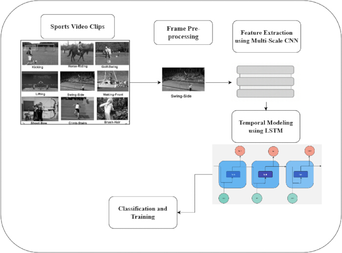
Figure 1: Proposed MSCNN-LSTM framework for sports video action recognition. Overall workflow illustrating video preprocessing, multi-scale spatial feature extraction, temporal sequence learning, and action classification. Please click here to view a larger version of this figure.

Figure 1 illustrates the workflow of the proposed sports video action-recognition framework based on a hybrid MSCNN-LSTM architecture. The process begins with sports video clips containing various athletic actions, including kicking, horse riding, and golf swinging. The raw videos were decomposed into individual frames during the preprocessing stage, where the frames are cropped, standardized, and prepared for model input. The preprocessed frames were then fed into the MSCNN module for feature extraction. The multi-scale convolutional architecture captures spatial features at different receptive fields, enabling the extraction of both local and contextual information from sports video frames. The extracted feature vectors were then processed by the LSTM network to model temporal dependencies and the evolution of motion across consecutive frames. Finally, the classification and training module used the learned spatiotemporal representations to predict the action category for each video clip. The proposed framework comprised four sequential steps, beginning with data collection and preprocessing using the UCF11 (YouTube Actions), UCF Sports, and JHMDB benchmark datasets. Each sports video was converted into a sequence of frames, which were resized, normalized, and augmented through rotation, flipping, and cropping to improve robustness to environmental variations. The preprocessed frames were then processed by the proposed Multi-Scale Convolutional Neural Network (MSCNN), where parallel convolutional branches with 3 × 3, 5 × 5, and 7 × 7 kernels extracted complementary local and contextual spatial features. These multi-scale features were concatenated and refined using batch normalization and max pooling to generate compact feature representations. The resulting frame-level features were subsequently provided to a Long Short-Term Memory (LSTM) network to model temporal dependencies across consecutive frames. The final LSTM outputs were flattened and passed through fully connected layers with ReLU activation, followed by a Softmax classifier to predict the action category. The network was trained using the Adam optimizer with a cross-entropy loss function and dropout regularization to reduce overfitting. Model performance was finally evaluated on the UCF11, UCF Sports, and JHMDB benchmark datasets using accuracy, precision, recall, and F1-score.

1. Data collection and pre-processing

Three publicly available benchmark datasets for sports and human action were used in this study. These datasets contain real-world sports footage with varying camera motion, viewpoints, and background complexity. Specifically, the study utilized UCF11 (YouTube Actions) (https://www.crcv.ucf.edu/data/UCF_YouTube_Action.php), which contains 11 action categories collected from 1,168 YouTube videos recorded from approximately 25 individuals, with multiple samples per action. The Joint-Annotated Human Motion Database (JHMDB)^34,35 contains 21 action classes and 928 annotated videos. The UCF Sports dataset comprises 10 action classes and 150 video sequences captured from broadcast sources with a resolution of 720 × 480 pixels (https://www.crcv.ucf.edu/data/UCF_Sports_Action.php).

Collectively, these datasets cover both individual and team sports and provide variation in temporal duration and visual scale for evaluating the proposed MSCNN-LSTM action-recognition framework. As part of the data-quality screening process, the UCF11, UCF Sports, and JHMDB datasets were examined for corrupted videos, duplicate files, and clips with incomplete annotations. No samples meeting these exclusion criteria were identified; therefore, all available videos were retained for subsequent analysis. The datasets were then partitioned into training (70%), validation (15%), and testing (15%) subsets using a consistent random-splitting strategy. Figure 2 presents representative images used for training and evaluation.

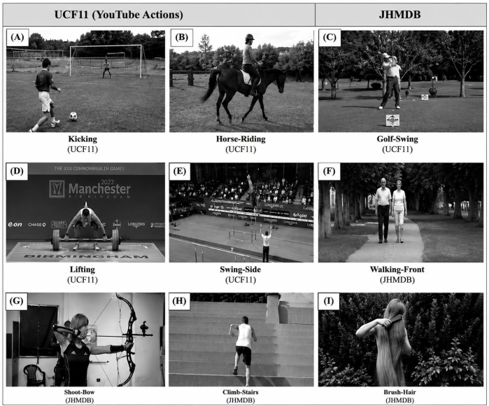
Figure 2: Representative frames from the benchmark sports action recognition datasets. Panels (A–D) show examples from the UCF11 (YouTube Actions) dataset, panels (E–H) from the UCF Sports dataset, and panels (I–L) from the JHMDB dataset. The frames illustrate variations in action classes, viewpoints, backgrounds, illumination conditions, and motion complexity. Please click here to view a larger version of this figure.

The proposed action-recognition model was evaluated on the UCF11, UCF Sports, and JHMDB benchmark datasets, as summarized in Table 3. These datasets represent diverse motion patterns and challenging environmental conditions. The UCF11 (YouTube Actions) dataset contains sports actions from 11 classes acquired under varying illumination, viewpoint, and background conditions. The UCF Sports dataset comprises 150 field-sports videos from professional broadcasts, featuring realistic motion sequences. The JHMDB dataset provides detailed human-motion annotations for 21 fine-grained action categories and serves as a benchmark dataset for spatiotemporal action recognition. Together, these datasets were used to evaluate model performance across sports and human-action scenarios. The network was trained using the Adam optimizer for 100 epochs with a batch size of 32, an initial learning rate of 0.001, and a cross-entropy loss function. The model with the lowest validation loss was selected for final evaluation. All experiments used a fixed random seed of 42. Early stopping and learning-rate reduction on plateau were applied to improve convergence, and gradient clipping with a threshold of 5.0 was used during LSTM training to prevent exploding gradients. The proposed MSCNN-LSTM model contained approximately 15 million trainable parameters. The hardware and software configuration used for implementation is summarized in Table 4. Because the class distributions were sufficiently balanced, no additional class-weighting or resampling procedures were applied. Comparator models were implemented using the hyperparameters reported in their original studies, with training settings harmonized where feasible. Performance values were reported as the mean ± standard deviation from five independent runs with different random initializations. Differences between the proposed model and the comparator models were evaluated using paired t-tests at a significance threshold of p < 0.05.

Dataset	No. of Classes	No. of Videos	Resolution (px)	Source	Description
UCF11 (YouTube Actions)	11	1168	Variable (≈ 320×240)	University of Central Florida	Includes 11 human actions from sports (e.g., basketball shooting, diving, golf swing, soccer juggling). Videos are collected from YouTube with high variation in illumination, viewpoint, and background.
UCF Sports	10	150	720×480	UCF Sports Action Dataset	Contains sports activities like diving, horse riding, golf swing, running, and weightlifting recorded from real broadcast TV footage (BBC, ESPN).
JHMDB	21	928	320×240	Max Planck Institute for Intelligent Systems	Includes daily and sports activities such as catching, jumping, brushing hair, shooting, and running with joint annotations for motion and pose analysis.

Table 3: Characteristics of the benchmark datasets used for training and evaluation. Overview of the UCF11, UCF Sports, and JHMDB datasets, including the number of action classes, video samples, dataset characteristics, and their roles in model training, validation, and testing.

Parameters Used	Description
Programming Language	Python 3.8.18 [4]
Deep Learning Framework	TensorFlow 2.15.0 [1]
GPU Accelerator	NVIDIA GeForce RTX 3090 (24 GB VRAM) [1]
CPU	Intel Core i9 @ 3.5 GHz × 16 Cores
Operating System	Windows 11
Memory (RAM)	64 GB DDR4
Optimizer	Adam (learning rate = 0.001)
Batch Size	32
Number of Epochs	100
Activation Functions	ReLU (CNN layers), Softmax (output layer)
Dropout Rate	0.5

Table 4: Simulation environment and hyperparameter configuration of the proposed MSCNN-LSTM model. Hardware specifications, software environment, optimizer settings, learning rate, batch size, number of epochs, input dimensions, and other hyperparameters used during model training and evaluation.

2. Pre-processing

Before training, each raw video was converted into a time-ordered sequence of frames and then normalized, temporally sampled, and augmented. Each input video V was first converted into a sequence of frames and represented as a 4D tensor V ∈ R^T×H×W×C, where T is the number of frames, H × W i denotes frame index, and C denotes the number of color channels (3 for RGB). The preprocessing pipeline consisted of frame extraction, spatial resizing followed by center or random cropping to a fixed resolution (H′, W′), per-pixel intensity normalization, and optional data augmentation, including random flipping, scaling, and color jittering, before feature extraction. Concretely, intensity normalization was implemented as either standard score normalization as in Eq. (1).

    (1)

where μ, σ are channel means and standard deviations computed over the training set, or as min–max scaling as in Eq. 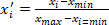(2).

    (2)

After normalization, each frame was represented as F̃_t ∈ R^{H′×W′×C′} and the resulting video tensor was represented as V′ ∈ R^{T×H′×W′×C}. In a multi-scale convolutional frontend, multiple receptive field spatial feature maps are obtained by applying several 2-D (or 3-D for early spatiotemporal convs) convolutions with different kernel sizes; a temporal feature representation was then generated for each frame or short video clip and forwarded to the LSTM module. The original paper applies the MobileNetV2 and then Deep BiLSTM for temporal modeling; the very same preprocessing pipeline above is fully compatible with a multi-scale conv + LSTM replacement.

3. Sampling and temporal normalization

Since video lengths T vary between and within datasets, we uniformly sample or temporally resample frames to give the multi-scale convolution + LSTM a fixed input length N in terms of frames or short snippets. Uniform frame indices can be computed as in Eq. (3),

(3)

so, the sampled frame sequence is V_s = {F̃_t0, …, F̃_tN−1}. When finer temporal fidelity is required, we perform linear temporal interpolation: for any resampled fractional time τ ∈ [0, T−1] computed as in Eq. (4).

(4)

so that the resampled sequence V_s has exactly N frames and preserves smooth motion. Alternatively, sampling by short contiguous clips (temporal window length w with stride s) yields a set of clip tensors where each clip C_j ∈ R^{T×H′×W′×C} and j = 0, …, ⌊(T − w)/s⌋. For temporal normalization inside the network, a simple temporal pooling at multiple scales is effective: given a temporal feature sequence X = {x₁, …, x_N} generated by multi-scale convs, apply pooled features as in Eq. (5).

(5)

where S_k is the temporal support for scale k (e.g., S_k may be non-overlapping blocks or dilated indices) and m_k = |S_k|.

Prior to feature extraction, all videos were scaled to 224 × 224 pixels and sampled at 25 frames per second. Every experiment employed a constant sequence length of 32 frames. Random cropping (scale = 0.8–1.0), random rotation (±15°), random horizontal flipping (probability = 0.5), and brightness modification (±20%) were among the data augmentation techniques. ImageNet mean values [0.485, 0.456, 0.406] and standard deviations [0.229, 0.224, 0.225] were used to standardize pixel values. For every video sequence, uniform frame selection was used for temporal sampling. Longer movies were uniformly trimmed or sampled to preserve a consistent sequence length, whereas videos with fewer than 32 frames were zero-padded. Throughout training and assessment, these settings were constantly used.

4. Feature extraction using MSCNN

A Multi-Scale Convolutional Neural Network (MSCNN) was employed to enhance the spatial representation of actions in sports videos. Conventional convolutional neural networks that rely on a single kernel size may have limited capability in capturing features at multiple spatial scales. Because some sports actions exhibit similar visual characteristics, it may be difficult for a single-scale convolutional architecture to simultaneously capture both local and global features. To address this limitation, the proposed framework utilizes convolutional kernels of different sizes to perform multi-scale feature extraction and feature fusion.

In the proposed network architecture, 1 × 1 convolution kernels were used to organize information across channels and to reduce the dimensionality of the input feature maps. In addition, these layers increase the expressive capability of the network by introducing additional feature transformations and nonlinear representations. Convolution kernels of different sizes enable the extraction of spatial information at multiple scales. Sequential normalization is performed following weighted multi-scale feature fusion to improve training stability. In order to mitigate gradient vanishing and gradient explosion problems during deep network training, the suggested architecture uses residual connections and LSTM-based temporal modeling.

The multi-scale design enhances the network's ability to capture features at different spatial resolutions and improves feature representation capability. Furthermore, the conventional N × N convolution kernel is decomposed into N × 1 and 1 × N convolution operations. The N × 1 and 1 × N convolutions employed in the MSCNN module are designed to capture complementary directional and multi-scale spatial features from individual video frames. These convolutional operations enhance spatial feature representation by extracting patterns at different receptive-field scales. Temporal relationships between consecutive frames are subsequently modeled by the LSTM module, which processes the sequence of MSCNN-extracted features to learn long-term temporal dependencies for action recognition.

Each sports video V = {F₁, F₂, …, F_T} is decomposed into T frames. To encode spatial variations, for example, player pose, motion blur, ball trajectory, convolutional branches at three different scales operate s ∈ {1, 2, 3}, corresponding to kernel sizes 3 × 3, 5 × 5 and 7 × 7. Each branch extracts feature maps as in Eq. (6):

    (6)

Where W_s and b_s are convolutional weights and biases at scale s, and σ is the ReLU activation. The multi-scale fusion layer aggregates features as in Eq. (7):

    (7)

This fused feature tensor embeds both fine-grained motion cues and large-area contextual information, such as group activities. Figure 3 illustrates only the MSCNN feature-extraction module. The LSTM layer (256 hidden units), dense layer (128 neurons), and dropout layer (0.5) used for temporal modeling and classification are presented separately in Figure 4.

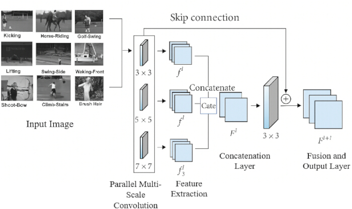
Figure 3: Proposed Multi-Scale Convolutional Neural Network (MSCNN) feature extraction module. Three parallel convolutional branches with kernel sizes of 3 × 3, 5 × 5, and 7 × 7 extract complementary multi-scale spatial features, which are fused before temporal modeling by the LSTM network. Please click here to view a larger version of this figure.

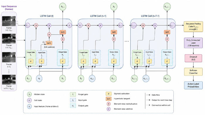
Figure 4: Proposed LSTM architecture for sports video action recognition. The LSTM module models temporal dependencies through input, forget, and output gate operations across consecutive video frames. Please click here to view a larger version of this figure.

Figure 3 illustrates the proposed Multi-Scale Convolutional Neural Network (MSCNN) feature extraction module for sports video action recognition. Input video frames were processed in parallel through three convolutional branches with kernel sizes of 3 × 3, 5 × 5, and 7 × 7, each containing 64 filters to capture complementary fine- and coarse-grained spatial features. The outputs were refined using Batch Normalization, ReLU activation, and 2 × 2 max pooling, then concatenated and fused by a 1 × 1 convolution with 128 filters. A residual skip connection preserved low-level spatial information and improved gradient flow. The fused feature maps were flattened and passed to an LSTM layer with 256 hidden units for temporal modeling, followed by a fully connected layer with 128 neurons, ReLU activation, and a dropout rate of 0.5 before final classification using a Softmax layer. The multi-scale feature maps (f₁^l, f₂^l, and f₃^l) were concatenated to form the fused representation (F^l), which was further refined by a 3 × 3 convolution to generate the output feature map for the subsequent layer. This hierarchical architecture enabled the learning of complementary spatial features at multiple receptive fields, improving sports action recognition performance.

5. Temporal modeling using LSTM

In order to model the time-based evolution across the video edges, the aggregated feature sequence was provided to the LSTM system to capture dynamic dependencies and continuity of motion. For each input video, we first extracted multiscale CNN features per frame. Let the video frames be I₁, …, I_T. For each frame t and each scale s the multi-scale convolutional encoder produces a feature vector f_t^(s) ∈ R^d. Then fuse scales into a single frame descriptor by either projection + concat or weighted sum as in Eq. (8):

     (8)

Then feed the sequence {x_t}_t^T=1 into an LSTM to model the temporal dynamics. In standard LSTM notation, at time t the gates and states are in Eq. (9) to (13):

(9)

(10)

(11)

(12)

(13)

Here σ is the sigmoid activation, ⊙ is element-wise multiplication.) Although bidirectional LSTM architectures can be used to capture both past and future temporal context, the proposed framework employs a standard LSTM to model temporal dependencies across sequential video frames. This design choice is consistent with the MSCNN-LSTM architecture presented in this study. After processing the clip, a clip representation was obtained (e.g., last hidden state or temporal pooling): z = Pool_t(v_t).

Figure 4 illustrates the workflow of the proposed LSTM architecture for sports action recognition. The network received a sequence of video frames or CNN-extracted features and processed them across successive time steps (t−2, t−1, and t). Each LSTM cell comprised an input gate, a forget gate, and an output gate, which regulated information flow through the network. The input gate incorporated new information into the cell state, the forget gate discarded irrelevant temporal information, and the output gate generated the hidden state propagated to the subsequent time step. The cell state preserved long-term temporal dependencies, whereas the hidden state captured short-term temporal information. After sequential processing, the LSTM outputs were pooled to generate a temporal feature representation, which was passed to a fully connected layer and a Softmax classifier to predict the corresponding sports action. The network was trained using the Adam optimizer for 100 epochs with a batch size of 32, an initial learning rate of 0.001, and a cross-entropy loss function. The model with the lowest validation loss was selected for final evaluation. To ensure reproducibility, all experiments were conducted using a fixed random seed of 42. Early stopping and learning-rate reduction on plateau were employed to improve convergence, and gradient clipping with a threshold of 5.0 was applied during LSTM training to prevent exploding gradients. The proposed MSCNN-LSTM model contained approximately 15 million trainable parameters.

The final class scores and probability uses a linear layer + softmax as in Eq. (14):

(14)

Train by minimizing the cross-entropy loss over the labeled clips as in Eq. (15):

(15)

where Nb is the size of the batch, C number of classes, and y⁽ⁿ⁾ is the one-hot ground truth. Regularization (dropout on x_t/LSTM outputs, weight decay) Gradient clipping is applied to help stability for long sports sequences.

Results

The proposed MSCNN-LSTM model was trained and evaluated on the UCF11 (YouTube Actions), UCF Sports, and JHMDB datasets, which included diverse sports actions, viewpoints, and motion patterns. Because the class distributions were sufficiently balanced, no additional class-weighting or resampling procedures were applied. Comparator models were implemented using the hyperparameters reported in their original studies, with training settings harmonized where feasible. Results were reported as the mean ± standard deviation from five independent runs with different random initializations. Differences between the proposed model and the comparator models were evaluated using paired t-tests at a significance threshold of p < 0.05.

Figure 5 compares classification accuracy across the three datasets. The MSCNN-LSTM model achieved the highest accuracy, reaching 98.3% on UCF11, 95.4% on UCF Sports, and 81.7% on JHMDB. These values exceeded those obtained by the Dilated CNN–BiLSTM, Two-Stream LSTM, and ViT-ReT models. The lower accuracy on JHMDB reflected the greater difficulty of recognizing fine-grained actions in lower-resolution videos.

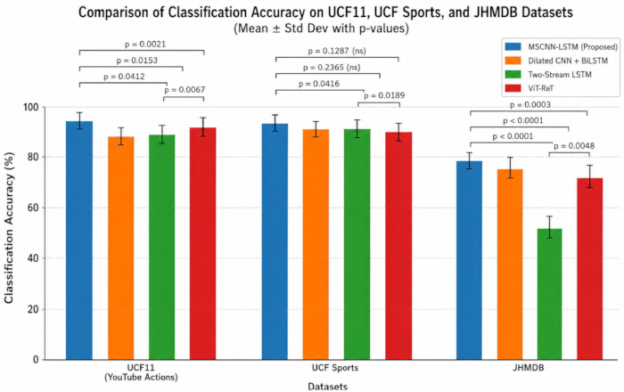
Figure 5: Comparison of classification accuracy (%) of different deep learning models on sports video datasets. Classification accuracy of MSCNN-LSTM, ViT-ReT, Two-Stream LSTM, and Dilated CNN + BiLSTM on the UCF11, UCF Sports, and JHMDB datasets. Results are reported as mean ± SD from five independent runs (n = 5). Error bars represent one standard deviation. Statistical significance was assessed using two-tailed paired t-tests (p < 0.05). Please click here to view a larger version of this figure.

The proposed model also achieved the highest precision across all datasets, with values of approximately 96% on UCF11, 93% on UCF Sports, and 78% on JHMDB (Figure 6). Recall values were approximately 95%, 94%, and 77%, respectively (Figure 7), while the corresponding F1-scores were approximately 95.5%, 93.5%, and 77.5% (Figure 8). These findings indicated that the model maintained a favorable balance between correctly identifying action classes and limiting false-positive predictions.

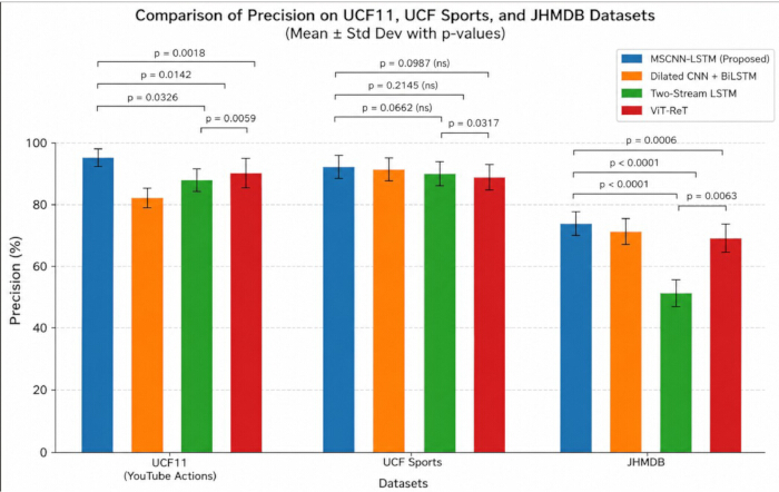
Figure 6: Comparison of precision (%) of different deep learning models on sports video datasets. Precision values are reported as mean ± SD from five independent runs (n = 5). Error bars represent one standard deviation. Statistical significance was assessed using two-tailed paired t-tests (p < 0.05). Please click here to view a larger version of this figure.

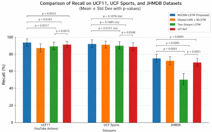
Figure 7: Comparison of recall (%) of different deep learning models on sports video datasets. Recall values are reported as mean ± SD from five independent runs (n = 5). Error bars represent one standard deviation. Statistical significance was assessed using two-tailed paired t-tests (p < 0.05). Please click here to view a larger version of this figure.

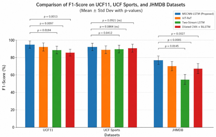
Figure 8: Comparison of F1-score (%) of different deep learning models on sports video datasets. F1-scores are reported as mean ± SD from five independent runs (n = 5). Error bars represent one standard deviation. Statistical significance was assessed using two-tailed paired t-tests (p < 0.05). Please click here to view a larger version of this figure.

Table 5 presents Cohen’s kappa and Matthews correlation coefficient results. On UCF11, the proposed model achieved κ = 0.96 and MCC = 0.96, compared with κ/MCC values of 0.92/0.92 for ViT-ReT, 0.90/0.90 for Two-Stream LSTM, and 0.87/0.87 for Dilated CNN–BiLSTM. On UCF Sports, the MSCNN-LSTM achieved κ = 0.95 and MCC = 0.94, exceeding the corresponding values obtained by ViT-ReT (0.90/0.90), Two-Stream LSTM (0.88/0.89), and Dilated CNN–BiLSTM (0.84/0.85). On JHMDB, the proposed model achieved κ = 0.83 and MCC = 0.84, compared with 0.74/0.75 for ViT-ReT, 0.70/0.71 for Two-Stream LSTM, and 0.71/0.72 for Dilated CNN–BiLSTM. These results showed stronger agreement between predicted and ground-truth labels for the proposed model.

Model	Dataset	Cohen’s Kappa (κ)	Matthews Correlation Coefficient (MCC)
Dilated CNN + BiLSTM [4]	UCF11 (YouTube Actions)	0.87 ± 0.01	0.88 ± 0.01
	UCF Sports	0.84 ± 0.02	0.85 ± 0.02
	JHMDB	0.71 ± 0.03	0.72 ± 0.03
Two-Stream LSTM [38]	UCF11 (YouTube Actions)	0.90 ± 0.01	0.91 ± 0.01
	UCF Sports	0.88 ± 0.02	0.89 ± 0.02
	JHMDB	0.70 ± 0.03	0.71 ± 0.03
ViT-ReT (Vision Transformer + Recurrent Transformer) [6]	UCF11 (YouTube Actions)	0.92 ± 0.01	0.92 ± 0.01
	UCF Sports	0.90 ± 0.01	0.90 ± 0.01
	JHMDB	0.74 ± 0.02	0.75 ± 0.02
Proposed MSCNN–LSTM	UCF11 (YouTube Actions)	0.96 ± 0.01	0.96 ± 0.01
	UCF Sports	0.95 ± 0.01	0.94 ± 0.01
	JHMDB	0.83 ± 0.02	0.84 ± 0.02

Table 5: Comparison of Cohen's kappa (κ) and Matthews correlation coefficient (MCC) across different deep learning models. Performance comparison of MSCNN-LSTM, ViT-ReT, Two-Stream LSTM, and Dilated CNN + BiLSTM on the UCF11, UCF Sports, and JHMDB datasets. Higher values indicate stronger agreement between predicted and true labels and greater classification reliability. Values are reported as mean ± SD from five independent runs (n = 5).

Figure 9 presents the receiver operating characteristic curves. The proposed MSCNN-LSTM achieved AUC values of 0.975 on UCF11, 0.961 on UCF Sports, and 0.937 on JHMDB. The consistently high AUC values indicated strong discrimination between action classes across datasets of differing complexity.

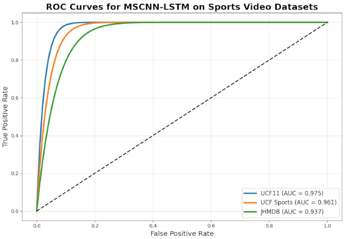
Figure 9: Receiver operating characteristic (ROC) curves of the proposed MSCNN-LSTM model. ROC curves for the UCF11, UCF Sports, and JHMDB datasets illustrating the trade-off between the true positive rate and false positive rate. The area under the curve (AUC) summarizes the discriminative performance of the model across classification thresholds. Please click here to view a larger version of this figure.

Temporal performance results are summarized in Table 6. On UCF11, the proposed model achieved an mAP-T of 98.3%, frame-level accuracy of 96.5%, and TSI of 0.95. On UCF Sports, the corresponding values were 95.4%, 94.0%, and 0.93. On JHMDB, the model achieved an mAP-T of 81.7%, frame-level accuracy of 78.9%, and TSI of 0.88 (Table 7). These values were higher than those obtained by the comparator models and indicated improved temporal coherence and prediction stability across both short- and long-duration action sequences.

Method	Dataset	mAP-T (%)	Frame-Level Accuracy (%)	Temporal Stability Index (TSI)
Dilated CNN + BiLSTM4	UCF11 (YouTube Actions)	93.6 ± 0.8	91.8 ± 0.9	0.87 ± 0.01
	UCF Sports	90.2 ± 1.0	89.1 ± 1.1	0.83 ± 0.02
	JHMDB	72.4 ± 1.5	70.3 ± 1.7	0.78 ± 0.03
Two-Stream LSTM38	UCF11 (YouTube Actions)	94.8 ± 0.7	92.6 ± 0.8	0.89 ± 0.01
	UCF Sports	91.3 ± 0.9	90.0 ± 1.0	0.85 ± 0.02
	JHMDB	73.8 ± 1.4	71.5 ± 1.6	0.79 ± 0.03
ViT-ReT (Vision Transformer + Recurrent Transformer)6	UCF11 (YouTube Actions)	95.5 ± 0.6	93.4 ± 0.7	0.90 ± 0.01
	UCF Sports	92.4 ± 0.8	91.2 ± 0.9	0.87 ± 0.01
	JHMDB	74.6 ± 1.3	72.8 ± 1.4	0.81 ± 0.02
.	UCF11 (YouTube Actions)	98.3 ± 0.5	96.5 ± 0.6	0.95 ± 0.01
	UCF Sports	95.4 ± 0.7	94.0 ± 0.8	0.93 ± 0.01
	JHMDB	81.7 ± 1.1	78.9 ± 1.3	0.88 ± 0.02

Table 6: Comparison of temporal performance metrics for sports video action recognition. Experimental results of mean Average Precision over Temporal Segments (mAP-T), frame-level accuracy, and Temporal Stability Index (TSI) for different deep learning models across the benchmark datasets. Values are reported as mean ± SD from five independent runs (n = 5).

Configuration	Multi-Scale CNN (MSCNN)	LSTM	Accuracy (%)	F1-Score (%)	mAP-T (%)
CNN-Only Baseline	✗	✗	90.4 ± 1.2	89.8 ± 1.3	88.9 ± 1.4
CNN + LSTM	✗	✓	93.1 ± 0.9	92.4 ± 1.0	91.7 ± 1.1
MSCNN Only	✓	✗	94.2 ± 0.8	93.6 ± 0.9	92.8 ± 1.0
Proposed MSCNN-LSTM	✓	✓	98.3 ± 0.5	97.8 ± 0.6	97.1 ± 0.6

Table 7: Ablation study of the proposed MSCNN-LSTM framework. Performance contribution of the MSCNN and LSTM components under identical training and evaluation settings. Values are reported as mean ± SD from five independent runs (n = 5).

Figure 10, Figure 11, Figure 12 present the row-normalized confusion matrices for UCF11, UCF Sports, and JHMDB, respectively. All three matrices showed clear diagonal dominance, indicating that most action classes were correctly identified. Limited off-diagonal errors occurred primarily between actions with similar visual or motion characteristics. The JHMDB matrix exhibited comparatively greater class confusion, consistent with the lower quantitative performance observed on this more challenging dataset.

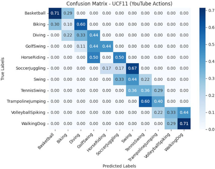
Figure 10: Row-normalized confusion matrix of the proposed MSCNN-LSTM model on the UCF11 dataset. Each row is normalized to unity, and diagonal entries represent class-wise recall rather than overall classification accuracy, which is reported separately. Please click here to view a larger version of this figure.

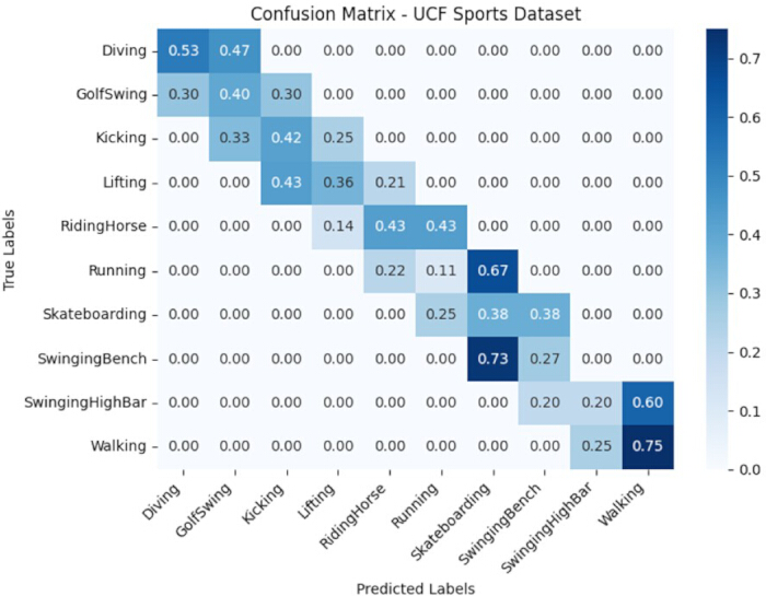
Figure 11: Row-normalized confusion matrix of the proposed MSCNN-LSTM model on the UCF Sports dataset. Each row is normalized to unity, and diagonal entries represent class-wise recall rather than overall classification accuracy, which is reported separately. Please click here to view a larger version of this figure.

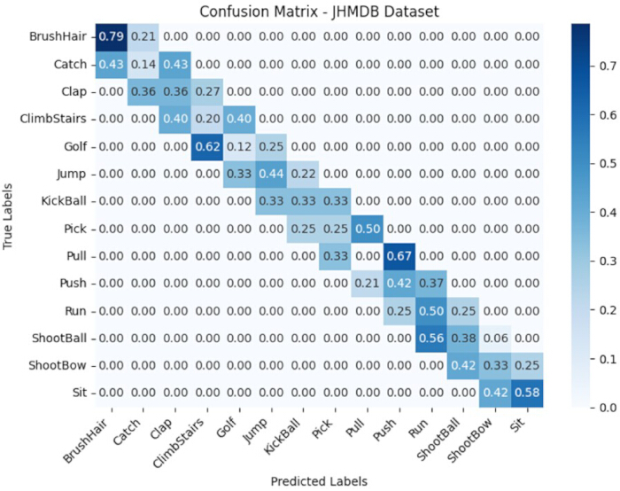
Figure 12: Row-normalized confusion matrix of the proposed MSCNN-LSTM model on the JHMDB dataset. Each row is normalized to unity, and diagonal entries represent class-wise recall rather than overall classification accuracy, which is reported separately. Please click here to view a larger version of this figure.

Overall, the proposed MSCNN-LSTM framework consistently outperformed the evaluated comparator models across classification, agreement, discrimination, and temporal-stability measures. The findings supported the hypothesis that combining multi-scale spatial feature extraction with LSTM-based temporal modeling improved sports action recognition across datasets with varying motion complexity, image quality, and viewpoint conditions.

DATA AVAILABILITY:

The datasets analysed during the current study are publicly available from the following sources: the UCF11 (YouTube Actions) dataset (https://www.crcv.ucf.edu/data/UCF_YouTube_Action.php) and the UCF Sports dataset (https://www.crcv.ucf.edu/data/UCF_Sports_Action.php). To support the reproducibility of this study, the preprocessing pipeline, dataset partitioning (train/validation/test split generation), implementation files, configuration files, and supporting documentation used in the experiments have been deposited in the Zenodo repository and are publicly available at https://doi.org/10.5281/zenodo.21020947.

Discussion

The proposed MSCNN-LSTM framework consistently outperformed the evaluated approaches across the UCF11, UCF Sports, and JHMDB benchmark datasets. Previous methods based on Dilated CNN–BiLSTM, Vision Transformer architectures, and 3D CNNs have demonstrated effective spatiotemporal feature learning but may be limited by high computational complexity, substantial training requirements, or insufficient representation of fine-grained motion patterns^23,24,25. In contrast, the proposed framework integrated multi-scale spatial feature extraction with LSTM-based temporal modeling, enabling the capture of both local motion details and long-range temporal dependencies. This integration improved the recognition of complex sports actions, reduced inter-class confusion, and enhanced temporal consistency, particularly on the more challenging JHMDB dataset. These findings indicate that the proposed framework provided a balanced representation of spatial and temporal information compared with the evaluated CNN-, recurrent-, and transformer-based approaches.

From a theoretical perspective, the MSCNN-LSTM framework provided a unified approach to multi-scale feature fusion and sequential temporal learning^36,37. The use of hierarchical receptive fields enabled the extraction of spatial information at different scales, while the LSTM modeled dependencies across consecutive video frames. This design extended the conventional CNN-LSTM pipeline by preserving local and contextual spatial information before temporal modeling. The consistent performance across datasets containing varied action classes, motion patterns, and camera viewpoints further supported the robustness of the proposed architecture.

From a practical perspective, the framework showed potential for automated sports analytics, athlete-performance assessment, event detection, and sports video understanding. However, further validation under real-world operating conditions is required before deployment. Although the architecture achieved strong recognition performance, its suitability for resource-constrained devices or cloud-based analytics platforms should be confirmed through additional evaluation of computational cost, inference time, memory requirements, and energy consumption.

The ablation study demonstrated the complementary contributions of the MSCNN and LSTM components. The MSCNN improved spatial feature extraction by learning representations at multiple receptive-field scales, whereas the LSTM enhanced temporal modeling by capturing motion dependencies across consecutive frames. The complete MSCNN-LSTM configuration achieved the best performance, indicating that multi-scale spatial feature extraction and temporal sequence modeling contributed jointly to the observed improvement in action recognition.

Overall, the proposed MSCNN-LSTM framework effectively combined spatial and temporal representation learning for sports video action recognition. Evaluation on the UCF11, UCF Sports, and JHMDB datasets showed improved performance compared with the evaluated deep learning approaches. These results supported the hypothesis that integrating multi-scale convolutional features with LSTM-based temporal modeling improves the recognition of complex sports actions. Nevertheless, validation on larger, more diverse, and cross-domain datasets is required to establish generalizability and real-world applicability.

Several limitations should be considered. First, the evaluation was restricted to publicly available benchmark datasets and may not fully represent the diversity and complexity of real-world sports environments. Second, although fixed training, validation, and test partitions were used, dataset bias and unintended data leakage could not be completely excluded. Third, reported performance may vary according to dataset composition, model initialization, preprocessing procedures, and training settings. In addition, the multi-scale convolutional and temporal modeling components increased computational requirements, which may affect deployment on devices with limited resources. The framework was also not evaluated using external datasets or real-time production scenarios.

Transformer-based video models have shown strong performance on large-scale action-recognition datasets but often require substantial computational resources and extensive training data. The proposed MSCNN-LSTM framework offers an alternative approach by combining multi-scale spatial feature extraction with recurrent temporal modeling. Future work should investigate cross-dataset validation, real-time inference, computational optimization, uncertainty estimation, and hybrid architectures that integrate transformer-based attention mechanisms with the proposed multi-scale CNN-LSTM framework³⁸.

Materials

List of materials used in this article

Name	Company	Catalog Number	Comments
GeForce RTX 3090 GPU	NVIDIA Corporation	RTX 3090, 24 GB VRAM	Used for deep learning model training and inference
Intel Core i9 Processor	Intel Corporation	16-Core, 3.5 GHz	Used for data preprocessing and computation
System Memory	Generic	64 GB DDR4 RAM	Supports large-scale video processing
Python Programming Language	Python Software Foundation	Version 3.8.18	Primary programming language for implementation
TensorFlow	Google	Version 2.15	Deep learning framework used for model development
Operating System	Microsoft Corporation	Windows 11	Model development and experimentation
CUDA Toolkit	NVIDIA Corporation	CUDA 11.8	GPU acceleration for model training
cuDNN	NVIDIA Corporation	cuDNN 8.9.7	Deep neural network acceleration library
OpenCV	Open Source	Version 4.8.1	Video frame extraction and preprocessing
NumPy	Open Source	Version 1.24.4	Numerical computation and array processing
Scikit-learn	Open Source	Version 1.3.2	Performance evaluation and statistical analysis
Matplotlib	Open Source	Version3.7.5	Visualization of experimental results
UCF11 Dataset	University of Central Florida	Public Dataset	Sports action recognition benchmark dataset
UCF Sports Dataset	University of Central Florida	Public Dataset	Sports action recognition benchmark dataset
JHMDB Dataset	Max Planck Institute for Informatics	Public Dataset	Human motion and action recognition benchmark dataset

References

- Hassan N, Miah ASM, Shin J. A deep bidirectional LSTM model enhanced by transfer-learning-based feature extraction for dynamic human activity recognition. Appl Sci. 2024;14:603. https://doi.org/10.3390/app14020603
- Egawa R, et al. Dynamic fall detection using graph-based spatial temporal convolution and attention network. Electronics. 2023;12:3234. https://doi.org/10.3390/electronics12153234
- Riahi M, Eslami M, Safavi SH, Torkamani Azar F. Human activity recognition using improved dynamic image. IET Image Process. 2020;14:3223–3231. https://doi.org/10.1049/iet-ipr.2020.0372
- Muhammad K, et al. Human action recognition using attention-based LSTM network with dilated CNN features. Future Gener Comput Syst. 2021;125:820–830. https://doi.org/10.1016/j.future.2021.06.017
- Al-Obaidi S, Al-Khafaji H, Abhayaratne C. Making sense of neuromorphic event data for human action recognition. IEEE Access. 2021;9:82686–82700. https://doi.org/10.1109/ACCESS.2021.3085769
- Wensel J, Ullah H, Munir A. ViT-ReT: Vision and recurrent transformer neural networks for human activity recognition in videos. IEEE Access. 2023;11:72227–72249. https://doi.org/10.1109/ACCESS.2023.3293445
- Vrskova R, Hudec R, Kamencay P, Sykora P. Human activity classification using the 3DCNN architecture. Appl Sci. 2022;12:931. https://doi.org/10.3390/app12020931
- Ullah A, et al. Action recognition using optimized deep autoencoder and CNN for surveillance data streams of non-stationary environments. Future Gener Comput Syst. 2019;96:386–397. https://doi.org/10.1016/j.future.2019.01.041
- Jaouedi N, Boujnah N, Bouhlel MS. A new hybrid deep learning model for human action recognition. J King Saud Univ Comput Inf Sci. 2020;32:447–453. https://doi.org/10.1016/j.jksuci.2018.08.001
- Zebhi S, Al-Modarresi SMT, Abootalebi V. Converting video classification problem to image classification with global descriptors and pre-trained network. IET Comput Vis. 2020;14:614–624. https://doi.org/10.1049/iet-cvi.2020.0023
- Cust E, Sweeting AJ, Ball K, Robertson S. Machine and deep learning for sport-specific movement recognition: A systematic review. J Sports Sci. 2019;37:568–600. https://doi.org/10.1080/02640414.2018.1504613
- Cao S, Wang B, Zhang W, Ma L. Visual consensus modeling for video-text retrieval. In Proc AAAI Conf Artif Intell. 2022:167–175. https://doi.org/10.1609/aaai.v36i1.19890
- Yu H, et al. Fine-grained video captioning for sports narrative. In Proc IEEE Conf Comput Vis Pattern Recognit (CVPR). 2018:6006–6015. https://doi.org/10.1109/CVPR.2018.00628
- Browne P, Sweeting AJ, Woods CT, Robertson S. Methodological considerations for furthering the understanding of constraints in applied sports. Sports Med Open. 2021;7:22. https://doi.org/10.1186/s40798-021-00307-9
- Gao T, et al. Sports video classification method based on improved deep learning. Appl Sci. 2024;14:948. https://doi.org/10.3390/app14020948
- Dong Z, Xie M, Li X. Multi-scale receptive fields convolutional network for action recognition. Appl Sci. 2023;13:3403. https://doi.org/10.3390/app13063403
- Liu S, et al. Human memory update strategy: A multi-layer template update mechanism for remote visual monitoring. IEEE Trans Multimed. 2021;23:2188–2198. https://doi.org/10.1109/TMM.2020.3009234
- Liu S, Liu D, Muhammad K, Ding W. Effective template update mechanism in visual tracking with background clutter. Neurocomputing. 2021;458:615–625. https://doi.org/10.1016/j.neucom.2021.05.032
- Haque MN, et al. GRU-based attention mechanism for human activity recognition. In Proc ICASERT. 2019:1–6. https://doi.org/10.1109/ICASERT.2019.8934521
- Al-qaness MA, Dahou A, AbdElaziz M, Helmi A. Multi-ResAtt: Multilevel residual network with attention for human activity recognition using wearable sensors. IEEE Trans Ind Inform. 2022;19:144–152. https://doi.org/10.1109/TII.2022.3147850
- Duan F, et al. A multi-task deep learning approach for sensor-based human activity recognition and segmentation. IEEE Trans Instrum Meas. 2023;72:2514012. https://doi.org/10.1109/TIM.2023.3264512
- Gomes E, et al. Machine learning algorithms for activity-intensity recognition using accelerometer data. Sensors. 2021;21:1214. https://doi.org/10.3390/s21041214
- Su C, et al. A novel model for fall detection and action recognition combining lightweight 3D-CNN and ConvLSTM networks. Pattern Anal Appl. 2024;27:3. https://doi.org/10.1007/s10044-023-01234-5
- Zhou T, et al. Behavior recognition based on improved density clustering and context-guided Bi-LSTM model. Multimed Tools Appl. 2023;82:45471–45488. https://doi.org/10.1007/s11042-023-14678-9
- Shin J, et al. Video-based human activity recognition using hybrid deep learning model. Comput Model Eng Sci. 2025;143:3615. https://doi.org/10.32604/cmes.2025.058341
- Vrskova R, Hudec R, Kamencay P, Sykora P. A new approach for abnormal human activities recognition based on ConvLSTM architecture. Sensors. 2022;22:2946. https://doi.org/10.3390/s22082946
- Vijeikis R, Raudonis V, Dervinis G. Efficient violence detection in surveillance. Sensors. 2022;22:2216. https://doi.org/10.3390/s22062216
- Rendón-Segador F, et al. ViolenceNet: Dense multi-head self-attention with bidirectional ConvLSTM for detecting violence. Electronics. 2021;10:1601. https://doi.org/10.3390/electronics10131601
- Kalfaoglu E, Kalkan S, Alatan A. Late temporal modeling in 3D CNN architectures with BERT for action recognition. In Proc ECCV Workshops. 2020. https://doi.org/10.1007/978-3-030-66823-5_43
- Moaaz M, Mohamed E. Violence detection in surveillance videos using deep learning. Inf Bull Fac Comput Artif Intell. 2020;2:6.
- Song W, et al. Expressive 3D facial animation generation based on local-to-global latent diffusion. IEEE Trans Vis Comput Graph. 2024;30:7397–7407. https://doi.org/10.1109/TVCG.2024.3456213
- Li L, Cherouat A, Snoussi H, Wang T. Grasping with occlusion-aware ally method in complex scenes. IEEE Trans Autom Sci Eng. 2025;22:5944–5954. https://doi.org/10.1109/TASE.2024.3434610
- Li R, et al. UE-Extractor: A grid-to-point ground extraction framework for unstructured environments. IEEE Robot Autom Lett. 2025;10:5991–5998. https://doi.org/10.1109/LRA.2025.3563127
- Jhuang, H., Gall, J., Zuffi, S., Schmid, C., Black, M. J. Towards understanding action recognition. Proceedings of the IEEE International Conference on Computer Vision. 3192–3199, doi:10.1109/ICCV.2013.396 (2013).
- OpenMMLab. MMAction2: JHMDB dataset preparation. GitHub. https://github.com/open-mmlab/mmaction2/tree/main/tools/data/jhmdb (2026).
- Ullah W, Khalid YN, Khan SH. A novel deep hybrid framework with ensemble-based feature optimization for HAR. arXiv preprint arXiv:2508.18695. 2025. https://arxiv.org/abs/2508.18695
- Karuppannan K, Darmanayagam SE, Cyril SR. Human action recognition using fusion-based discriminative features and LSTM classification. Concurr Comput Pract Exp. 2022;34:e7250. https://doi.org/10.1002/cpe.7250
- Sahoo SP, et al. HAR-depth: A novel framework for human action recognition using sequential learning and depth estimated history images. IEEE Trans Emerg Top Comput Intell. 2020;5:813–825. https://doi.org/10.1109/TETCI.2020.3006543