A Semantic Parsing Method for Indoor Scene Images Based on Prior Knowledge of Building Structure

Summary

This study proposes an algorithm that tightly couples the hierarchical visual features captured by a shifted-window hierarchical transformer encoder with the prior depth of the Manhattan 3D bounding box generated by line-segment detection, thereby achieving high-precision semantic reconstruction of complex indoor scenes.

Abstract

To address semantic prediction discontinuities and physical boundary distortions caused by furniture occlusion in complex indoor scenes, this paper proposes a semantic parsing method that leverages building-structure priors. The scheme uses a shifted-window hierarchical transformer encoder to extract multi-scale visual features and combines a gradient-direction-consistency line segment detection algorithm to construct a Manhattan 3D bounding box. This bounding box is transformed into a signed distance field (SDF) prior to encoding discrete geometric contours into a continuous physical potential field. A structure-guided cross-attention mechanism forces the visual signals to align with real 3D orthogonal geometric boundaries, restoring feature continuity in occluded areas. A spatial adjacency graph constructed from superpixel nodes drives a Graph Convolutional Network (GCN) to aggregate features, ensuring macroscopic semantic consistency within the physical load-bearing plane. A combination of pixel-level cross-entropy loss and a custom-designed structural consistency loss strengthens the constraints, penalizing out-of-bounds predictions. Experiments across multiple independent runs show that the mean intersection over union (mIoU) reaches 68.7% with a standard deviation of 0.2%, and the structural boundary F1 score reaches 76.4% with a standard deviation of 0.3%, confirming the robust performance of the proposed modules. With a single image node size of 256, the average inference time remained at 61 ms.

Introduction

Indoor scene image semantic analysis occupies a core position in three-dimensional spatial cognition and intelligent spatial reasoning tasks^1,2. Visual feature extraction in real physical environments is often severely hindered by complex spatial layouts³. Solving the semantic discontinuity and physical boundary distortion of the building foundation structure building foundation structure caused by large-scale furniture occlusion is important for spatial cognition research^4,5. Accurately removing interference from cluttered objects and restoring the physical continuity of the same wall and floor will directly determine the accuracy of three-dimensional scene reconstruction and global spatial logic analysis⁶. The semantic discontinuity caused by large-scale furniture occlusion and the structural repair effect of the proposed building-prior guidance are illustrated in Figure 1, where the occluded red green blue (RGB) input in Table 1A, baseline mask distortion in Figure 1B, and structure-prior repair result in Figure 1C are compared under the same indoor scene condition.

To meet the accuracy requirements of spatial logical reasoning, current mainstream pixel-driven visual networks face multiple obstacles when dealing with complex indoor environments^7,8. Indoor spaces are often filled with dense furniture and cluttered furnishings, resulting in a significant loss of low-level visual boundary signals in the images⁹. Conventional feature extraction mechanisms rely excessively on local two-dimensional color and texture responses, lacking a macroscopic understanding of the rigid orthogonal laws of three-dimensional man-made structures¹⁰. This limitation of the local receptive field makes feature propagation easily interrupted, making it difficult to extend the global topology across occlusions¹¹. Currently, there is an urgent need to solve the core problem of semantic prediction discontinuities and severe distortions of physical boundaries caused by occlusion and interference¹².

To address structural faults in building foundations caused by occlusion and interference, the academic community has developed a variety of targeted intervention measures¹³. Cross-modal feature aggregation networks effectively compensate for the inherent deficiencies of a single visual modality in spatial perception by introducing depth maps or text priors to assist with red-green-blue (RGB) images^14,15. Boundary perception and adaptive context selection frameworks inject physical contour enhancement strategies into the feature decoding stage, which greatly improves the edge fit of prediction results in complex scenes^16,17. Inference models based on GCNs and feature interaction mechanisms significantly improve feature smoothness and macro-semantic consistency in homogeneous regions by constructing node-level connections^18,19. Integrating explicit Manhattan structural priors into the visual feature extraction pipeline enforces geometric consistency boundaries, which addresses the feature discontinuity challenges caused by extensive foreground object occlusion²⁰.

To address the core challenge of semantic prediction faults and severe distortions of physical boundaries associated with building infrastructure, a semantic parsing framework is proposed based on a closed-loop coupling mechanism incorporating architectural priors. This framework transcends naive engineering pipelines by establishing a bidirectional mapping alignment between continuous geometric potential fields and discrete visual feature manifolds, forming a non-trivial synergy that rectifies occlusion errors through structural laws. This scheme relies on a multi-scale visual backbone network and a line-segment detection algorithm based on vanishing-point estimation to acquire local appearance features and orthogonal edge priors that represent the Manhattan 3D bounding box in parallel, and then transform them into an SDF. The algorithm employs a structure-guided cross-attention mechanism, using visual features as query vectors and treating SDF features as keys and values for dot-product calculations, thereby forcing the visual signal to align with the real 3D geometric boundary in the feature space. A spatial adjacency graph constructed from superpixel nodes and spatial coplanarity edge features is fed into a GCN to perform cross-node feature aggregation and message passing. The end-to-end parameter optimization process jointly employs pixel-level cross-entropy and a custom structural consistency loss function, which strictly constrains and penalizes predicted pixels that cross the building-prior boundary. The complete semantic parsing pipeline is summarized in Figure 2, which links RGB image input, geometric prior extraction, cross-attention alignment, superpixel graph reasoning, and semantic mask decoding within a unified architecture.

Early scene parsing networks relied on convolutional operations to capture local appearance textures, but due to limitations in local receptive fields, they exhibited insufficient semantic coherence of large-scale targets^21,22. Previous studies have applied the self-attention module of the visual Transformer architecture to extract global contextual information and construct long-distance pixel association features^23,24. Cross-modal multi-view feature aggregation strategies extract the three-dimensional geometric spatial features of the scene by fusing depth-map point clouds and text command inputs^25,26. Hybrid attention mechanisms for feature fusion targeting specific domains have gradually matured. By constructing feature interaction bridges, they have significantly reduced energy loss and feature sparsity in multi-scale transmission of visual signals and improved the robustness of complex-structure parsing. Cutting-edge encoder designs jointly integrate and infer high-frequency domain spatial details alongside global and local features, strengthening the network's ability to distinguish fine-grained semantic categories with high similarity and improving indoor parsing accuracy^27,28. Recent advancements in semantic segmentation architectures provide valuable references for optimizing computational efficiency and spatial perception. Models designed for dense prediction and multi-scale contextual aggregation extract fine-grained geometric features from complex backgrounds. Feature decoupling and synergistic fusion strategies address the semantic ambiguity in boundary regions. Lightweight attention mechanisms and gated aggregation modules optimize the parameter distribution, thereby accelerating inference while preserving local structural details. Implementing these efficient architectural designs offers theoretical guidance for reducing the computational overhead of non-Euclidean topological inference operations in indoor scene parsing.

Building structure priors and 3D layout estimation are used to correct local visual parsing errors²⁹. Previous studies have extracted orthogonal and parallel geometric features of indoor buildings as inference constraints to reduce network prediction bias caused by cluttered indoor backgrounds^30,31. Existing schemes use line segment detection algorithms and image ablation point analysis techniques to generate Manhattan 3D bounding boxes to map the physical boundaries of rooms and assist in the localization of underlying visual features³². The joint architecture of the boundary awareness module and the multi-scale context implicitly embeds prior structural information into the high-dimensional feature decoding process, forcing the network to output semantic masks that closely match the real physical contours, effectively improving the jaggedness and blurring of object edges³³. Semi-supervised or weakly supervised loss function designs with boundary enhancement properties have been widely explored. Relying on rigorous mathematical formulas to punish independent pixel classification behavior that violates spatial topological rules, the geometric smoothness and structural integrity of the final segmentation result are guaranteed from the source of gradient optimization³⁴.

Some studies have used graph neural networks to perform cross-domain aggregation of visual features and reasoning about topological relationships in high-dimensional space³⁵. The superpixel segmentation algorithm pre-aggregates adjacent pixel blocks with similar color response and texture features into independent connected nodes. The superpixel segmentation algorithm compresses the computational redundancy of the graph structure at the image level and preserves the basic geometric topology of the image³⁶. The GCN built on the high-dimensional node feature vector, and the adjacency matrix representing spatial proximity drives the efficient directional transmission and interactive fusion of multi-scale visual information along the physical connected graph in the spatial domain^37,38. The application of the temporal information enhancement module and the hybrid multi-scale skip connection mechanism suppresses the excessive smoothing and homogenization of node features generated in the process of multi-layer deep message passing³⁹. The multi-scale graph wavelet transform technology, and the pseudo-label element learning optimization strategy optimize the anti-background noise mechanism of the node feature update formula, so that features with the same semantic attributes maintain a cooperative response mode in complex network topology⁴⁰. The graph-based reasoning mechanism maps regular pixel grids to non-Euclidean topological spaces to perform feature aggregation calculations of irregular building structures and interior components⁴¹.

Protocol

Indoor RGB scene datasets and their semantic annotations were prepared prior to network training. The large-scale indoor 3D dataset and RGB-D indoor scene dataset (see the Table of Materials) were obtained from their official repositories. Indoor acquisition scenes containing furniture occlusion, illumination variation, wall boundary interruption, and complex spatial layouts were retained to match the target parsing scenario. Semantic labels were converted into indexed single-channel PNG annotation masks, and all RGB images and semantic masks were resized to 512 × 512 pixels. Online data augmentation was applied during training, with random horizontal flipping at a probability of 0.5, random brightness scaling between 0.8 and 1.2, and random rotation between −10° and +10° to broaden the structural layout distribution. RGB channels were normalized with mean values of 0.485, 0.456, and 0.406 and standard deviation values of 0.229, 0.224, and 0.225. The large-scale indoor 3D benchmark followed the official release split used in this study, with 1201 training scenes and 312 validation scenes for model development and validation. The RGB-D indoor scene benchmark followed the official evaluation protocol, with 795 training images and 654 testing images. No additional percentage-based split was applied to these two public benchmarks.

A shifted-window hierarchical transformer visual backbone network (see the Table of Materials) was initialized as the moving-window transformer encoder backbone. The patch embedding size was configured as 4 x 4 pixels. The embedding dimensions of the four hierarchical stages were set to 128, 256, 512, and 1024, and the number of transformer blocks in the four stages was set to 2, 2, 18, and 2. The local attention window size was set to 7 x 7, and the number of attention heads was set to 4, 8, 16, and 32 for the four hierarchical stages. Nonlinear continuous activation functions were used inside all multilayer perceptron layers. Spatial downsampling was performed through patch-merging operations with a stride of 2 after each hierarchical stage. The core network architecture and convolutional inference module hyperparameters were summarized in Table 1.

Shifted-window self-attention feature extraction was then performed on the input feature maps. Each feature map was divided into non-overlapping local windows with spatial dimensions of 7 × 7. Regular window attention and shifted-window attention were alternated between adjacent shifted-window transformer blocks. The cyclic shift distance was set to 3 pixels, and relative positional bias encoding was applied within each local attention window. Local visual features were aggregated via multi-head self-attention to generate hierarchical, multi-scale feature representations.

Manhattan structural priors were extracted from indoor RGB images. Structural edge segments were detected using a gradient-direction-consistency line segment detection algorithm. Dominant structural directions were clustered through a random sample consensus (RANSAC) algorithm (see the Table of Materials) based on vanishing-point estimation. Three mutually orthogonal Manhattan directions were reconstructed to generate the Manhattan 3D bounding box representation. The reconstructed structural boundary was converted into an SDF map by computing the minimum Euclidean distance from each pixel to the nearest boundary line segment.

Structure-guided cross-attention features were generated after the visual features and SDF priors had been obtained. The visual feature manifold was mapped to the query tensor Q through the linear transformation matrix W sub Q element of double-struck cap R to the formation matrix W sub Q element of double-struck cap R to the formation matrix 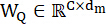. The continuous distance field prior was mapped to the key tensor K and the value tensor V through the transformation matrices , and the model dimension was set to 512. Multi-head modulation divided the projection space into 8 independent subspaces, with each head having a dimension of 64. The spatial layout prior projected discrete pixel coordinates into a continuous potential field and generated the structural affinity matrix S as an explicit additive spatial bias for modulating the dot-product similarity matrix. The visual feature tensor was used as the query source because semantic parsing requires each visual location to actively retrieve structurally consistent evidence from the geometric prior space. The SDF prior was used as the key and value source because it stores continuous boundary distance and inside-outside structural cues derived from the Manhattan layout. The dot-product term measured the compatibility between the semantic appearance and the geometric prior, while the additive structural term λS shifted attention weights toward pixels on the same physical plane or near the same architectural contour. The coefficient λ represented the confidence in the extracted structural prior and controlled the extent to which rigid orthogonal constraints were incorporated into the attention distribution. This formulation reduced cross-boundary feature diffusion caused by furniture occlusion and retained adaptive relaxation in non-Manhattan layouts. The structure-guided attention distribution was calculated according to Equation 1.

Equation 1:

where A denotes the structure-guided attention aggregation matrix, Q denotes the query tensor generated from visual features, K denotes the key tensor generated from SDF prior features, V denotes the value tensor generated from structural prior representations, dk denotes the feature dimension of the key tensor, λ denotes the adaptive structural weighting coefficient used to identify the geometric confidence of local regions and relax rigid orthogonal constraints in non-Manhattan spatial layouts, and S denotes the SDF affinity matrix. The division by dk stabilized the scale of attention logits and prevented large feature dimensions from producing over-concentrated attention weights. The normalized exponential function (see the Table of Materials) transformed the modulated similarity scores into a normalized spatial distribution, allowing each pixel to aggregate structural prior information based on semantic and geometric consistency. This design explains why visual appearance and architectural boundary priors are fused at the attention level rather than by direct feature concatenation.

The superpixel topology graph was constructed from the structure-aligned feature map. The feature map was segmented using a spatial region generation algorithm. The superpixel number was set to 256, the compactness coefficient was set to 10, the Gaussian smoothing coefficient was set to 1.0, and the iteration number was set to 10. Spatial proximity constraints were enforced by setting the distance metric weight to a constant ratio of 1.0 to the feature color-space distance during clustering, thereby maintaining uniform node generation across dense clutter boundaries. Pixels with homogeneous semantic responses were aggregated into superpixel nodes. Graph edges were constructed according to spatial adjacency relationships, SDF affinity strength, and coplanar geometric consistency constraints. The construction process of the structural affinity matrix and topological connectivity is shown in Figure 3, presenting how SDF guidance was transformed into graph-level spatial relationships.

The graph formulation was introduced to convert dense pixel-wise reasoning into node-wise spatial reasoning over homogeneous structural regions. Each superpixel node represented a local region with similar semantic response and spatial continuity, while each edge represented a reliable path for feature transmission subject to adjacency, distance-field affinity, and coplanar-consistency constraints. This design reduced the influence of isolated noisy pixels and enabled occluded wall, floor, and ceiling regions to receive messages from physically adjacent nodes. The edge construction, therefore, served as a mathematical bridge between continuous SDF guidance and discrete non-Euclidean graph reasoning.

A three-layer graph convolutional reasoning network was configured with hidden feature dimensions of 512, 256, and 128. The graph convolutional layer performed feature smoothing over the graph structure based on the nodes' spatial relationships. The self-loop adjacency retained each node's original state during message passing, preventing the features of a small structural region from being erased by surrounding large regions. Symmetric normalization scaled the adjacency matrix elements by the product of the inverse square roots of the node degrees so that high-degree nodes and low-degree nodes contributed under comparable numerical magnitudes during propagation. Feed-forward propagation performed localized spatial aggregation, in which each node state absorbed high-dimensional features from adjacent coplanar clusters before the element-wise nonlinear rectification function was applied. This formulation made the graph convolution layer approximate semantic diffusion along physically meaningful indoor planes rather than unrestricted smoothing across the boundaries of unrelated objects. Graph node features were evaluated according to Equation 2.

Equation 2:

The projection from dense pixel features to superpixel nodes, graph-convolution message passing, and coordinate back-projection are presented in Figure 4, clarifying the feature-aggregation path from regular image grids to a non-Euclidean topology and back to a dense semantic representation. The projection from dense pixel features in Figure 4A to superpixel nodes in Figure 4B, graph-convolution message passing in Figure 4C, and coordinate back-projection in Figure 4D clarify the feature-aggregation path from regular image grids to a non-Euclidean topology and back to a dense semantic representation.

where H(l) denotes the node feature tensor of the l-th graph convolution layer, Â denotes the adjacency matrix with self-loop connections, D denotes the degree matrix corresponding to the adjacency matrix, W(l) denotes the learnable weight matrix of the l-th graph convolution layer, and σ denotes the Rectified Linear Unit activation function. The term ÂH(l) aggregated features from adjacent superpixel nodes, while D^−1/2 and D^−1/2 balanced the contribution of nodes with different connection densities. The learnable matrix W(l) projected aggregated node features into a new semantic space, allowing the graph layer to distinguish structural consistency from ordinary spatial closeness. The nonlinear activation preserved the difference in responses between coplanar and non-coplanar regions after feature aggregation.

Semantic segmentation features were decoded after graph reasoning. The decoder was constructed using three bilinear interpolation upsampling stages and cross-layer skip-connection fusion operations. Shallow spatial encoder features were concatenated with high-level semantic decoder features through channel-wise fusion. The feature resolution was restored to the original image size, and the final semantic probability prediction map was generated through a 1 × 1 convolution layer.

The full semantic parsing network was trained using a decoupled weight-decay optimizer (see the Table of Materials). The initial learning rate was set to 0.0001, the weight decay coefficient to 0.01, and the batch size to 8 for both public benchmarks. The first moment decay rate was set to 0.9, the second moment decay rate was set to 0.999, and the numerical stability epsilon coefficient was set to 1 × 10⁻⁸. The validation loss was monitored at the end of each epoch, and checkpoints were saved when the mIoU on the validation set increased. The network was trained for 300 epochs using a polynomial learning rate decay strategy with a decay power of 0.9. Five independent training runs were conducted using different random-seed initializations to establish a statistically rigorous evaluation baseline. The network was jointly optimized using pixel-level cross-entropy loss and structural consistency loss. All experiments were performed on a computing platform equipped with high-memory parallel computing hardware, and detailed hardware information was reported in the Table of Materials.

Joint optimization enforced geometric boundary alignment by computing the spatial gradient magnitude of the class probability tensor. The structural consistency loss was used as a regularizer, multiplying the norm of the spatial prediction gradients by the continuous SDF values. The mathematical rationale was that semantic category changes should concentrate near real architectural contours, where the SDF approaches zero, while flat wall, floor, and ceiling interiors should maintain smooth semantic responses. When a large prediction gradient appeared far from a structural boundary, the distance field term increased the penalty and discouraged false semantic transitions inside a homogeneous physical plane. When a prediction gradient appeared near a zero-distance contour, the penalty remained limited and preserved legitimate class transitions along architectural boundaries. Semantic transition regions were constrained to align with the zero-distance contours of the SDF, as given by Equation 3.

Equation 3:

where L_total denotes the final optimization objective function, L_ce denotes the pixel-level cross-entropy loss, L_scl denotes the structural consistency penalty loss, and α denotes the structural loss weighting coefficient. The cross-entropy term provided pixel-level semantic supervision via annotation masks, while the structural consistency term imposed geometric regularization using architectural priors. The weighting coefficient α balanced category recognition and boundary alignment, preventing the optimization from overfitting either local label accuracy or rigid structural contours. This joint objective linked visual semantics, physical boundary consistency, and trainable network parameters within a unified optimization target.

Results

Experimental Setup

This study used two standard indoor scene parsing datasets, a large-scale indoor 3D dataset and an RGB-D indoor scene dataset, to evaluate performance and tune the model. The large-scale indoor 3D dataset contains realistically scanned, complex physical-space scenes and high-resolution RGB views, providing high-precision, pixel-by-pixel 3D point-cloud semantic labels and 2D spatial-projection segmentation masks. Its inherently realistic physical-space grid reconstruction data and orthogonal-plane properties establish a geometric-truth comparison criterion for accurately constructing the Manhattan 3D bounding box in the extraction branch. The RGB-D indoor scene dataset contains indoor depth images obscured by furniture and clutter and is used to test the network's global logical reasoning accuracy and robustness to occlusions.

The algorithm uses mIoU to measure the spatial overlap between the predicted and true semantic distributions, while also introducing a structural boundary F1 score to rigorously assess the accuracy of the fit between the predicted mask and the zero-distance physical-structure edges calibrated by the SDF. A fixed pixel-distance error threshold in Euclidean space is set during the calculation to determine whether the edge pixels produced by the network intersect the true physical boundary contours of the buildings. This dual evaluation system constrains classification errors in large-area semantic blocks while strengthening micro-quantitative assessment of the topological reconstruction effect of rigid lines. To maintain consistency between the experimental data configuration and the optimization process, the dataset scale and core training hyperparameters were summarized in Table 2. Table 2 reports one authoritative experimental configuration for the revised manuscript. The large-scale indoor 3D benchmark uses 1201 training scenes and 312 validation scenes, the RGB-D indoor scene benchmark uses 795 training images and 654 testing images, and both benchmarks are trained with a batch size of 8, an initial learning rate of 0.0001, a weight decay coefficient of 0.01, and 300 training epochs.

Comparison with state-of-the-art methods

Before presenting a quantitative comparison table of indoor scene parsing algorithms, this section rigorously defines the test benchmarks used in the multidimensional evaluation system. To reflect the model's classification performance at different granularities, the evaluation system supplements the test system with two additional metrics: global pixel accuracy (PixelAcc) and mean class accuracy (MeanAcc). These metrics together construct a detailed algorithm performance verification system, establishing a rigorous theoretical reference for subsequent quantitative analysis. To evaluate the semantic parsing accuracy and occlusion robustness of the proposed algorithm in complex physical spaces, comparative tests were conducted with existing algorithms on the RGB-D indoor scene validation set. The comparison model library covers foundational mask-attention frameworks, hierarchical vision Transformers, modern pure convolutional segmentation pipelines, unified dense-prediction architectures, and cross-channel attention networks. The benchmark evaluation was expanded to include a transformer-based segmentation baseline, a unified dense-prediction baseline, a unified detection and segmentation baseline, a large-scale vision foundation baseline, a pure convolutional baseline, a mask-attention-based segmentation baseline, a cross-modal feature aggregation baseline, and a progressive feature fusion baseline (see the Table of Materials), using the same RGB-D indoor scene validation set, input resolution, training schedule, and metric protocol. In the proposed architecture, the structure-guided network integrates a shifted-window multi-scale visual backbone, a structure-guided cross-attention module with an SDF, and a superpixel GCN. The expanded comparison covers transformer-based dense prediction, convolution-based dense prediction, mask-attention parsing, cross-modal feature fusion, and progressive feature fusion paradigms, enabling evaluation of the contribution of explicit 3D geometric boundary intervention against broader indoor scene parsing baselines.

Table 3 details the objective evaluation performance of each network on the core quantitative metrics, reporting the mean values and corresponding standard deviations across five independent runs. The expanded baseline comparison evaluates whether the proposed structure-guided reasoning mechanism contributes to accuracy gains beyond standard dense prediction backbones, mask-based segmentation networks, and RGB-D feature fusion networks. Experimental data show that the proposed algorithm achieves stable gains across all four quantitative metrics. Transformer-based dense prediction networks and mask-attention networks retained strong global context modeling ability, yet their Boundary F1 values remained lower in the presence of foreground clutter because the predicted masks lacked explicit physical boundary constraints. Cross-modal and progressive fusion networks improved local semantic continuity, but their feature fusion still relied primarily on appearance and depth responses rather than on a signed-distance structural prior. The proposed structure-guided network achieved a mIoU of 0.687 with a standard deviation of 0.002 and a mean Boundary F1 score of 0.764 with a standard deviation of 0.003. The expanded comparison indicates that the performance gain was not due solely to a larger dense prediction backbone, but rather to the joint use of signed-distance field guidance, structure-aware cross-attention, and graph-based topology reasoning.

To analyze the model's global logical reasoning accuracy under occlusions, we identified and extracted typical scenarios in the validation set that were severely obstructed by furniture and other clutter, and produced visualizations of pixel-level prediction masks.

After the method workflow and graph reasoning process were defined in Figure 1, Figure 2, Figure 3, and Figure 4. Figure 5 illustrates the differences in morphological predictions across models under extreme occlusion conditions. The red rectangles in the qualitative comparison mesh map mark key conflict areas where corners and load-bearing surfaces are occluded. The output mask from the mask-attention-based segmentation baseline shows pronounced edge smoothing and inter-class adhesion. Although the cross-modal feature aggregation baseline and the progressive feature fusion baseline incorporate cross-modal data, their prediction results still exhibit structural class discontinuities and physical boundary distortions. The mask generated by this proposed method exhibits high spatial overlap with the ground-truth labels. Baseline models, constrained by purely pixel-driven principles, are prone to losing their local receptive fields when occluded. The proposed method uses a superpixel GCN to perform message passing in non-Euclidean space, thereby reconstructing the underlying corners and linear spatial skeletons guided by implicit geometric boundaries. This verifies the anti-interference performance of our proposed solution in resolving complex indoor layouts from a visual morphological perspective.

Ablation experiment

To analyze the actual contribution of each independent component in the proposed architecture, this study constructed an expanded modular ablation test on the RGB-D indoor scene validation set. The test baseline was set to a conventional classification network with only the base shifted-window transformer visual backbone. Quantitative evaluation measured the independent contribution of structure-guided cross-attention, signed-distance field bias, adaptive structural weighting, superpixel graph reasoning, coplanar edge construction, symmetric graph normalization, and structural consistency loss. This expanded ablation design separated cumulative module gains from component-removal effects, making the contribution boundary of each design choice clearer.

Table 4 and Figure 6 illustrate the evolution of accuracy under expanded cumulative and removal-based ablation settings. The base shifted-window transformer network lacks three-dimensional physical boundary constraints, resulting in limited feature aggregation in cluttered backgrounds. Adding structure-guided cross-attention increased the mIoU from 0.615 to 0.648 and the Boundary F1 score from 0.630 to 0.685, showing that the signed-distance field prior improved the alignment between visual features and structural contours. Adding superpixel graph reasoning alone increased the mIoU to 0.641 and the Boundary F1 score to 0.676, indicating that node-wise topology reasoning improved semantic consistency over homogeneous physical regions. Adding structural consistency loss alone increased the mIoU to 0.632 and the Boundary F1 score to 0.662, showing that the loss term mainly affected boundary fitting rather than broad contextual aggregation.

Combining cross-attention with graph reasoning increased the mIoU to 0.669 and the Boundary F1 score to 0.721, showing that visual-structural alignment and graph-domain message passing produced complementary effects. Combining cross-attention with structural consistency loss achieved a mIoU of 0.660 and a Boundary F1 score of 0.713, while combining graph reasoning with structural consistency loss achieved a mIoU of 0.653 and a Boundary F1 score of 0.704. These pairwise results indicate that the cross-attention module provided the main geometric alignment signal, the graph reasoning module expanded this signal across coplanar regions, and the structural consistency loss refined the semantic transition boundary during optimization.

Removal-based ablation further clarified the contribution of the internal design choices. Removing the signed-distance field additive bias reduced the mIoU to 0.656 and the Boundary F1 score to 0.698, confirming that the structural affinity matrix was central to suppressing cross-boundary feature diffusion. Removing the adaptive structural weighting coefficient λ reduced the mIoU to 0.671 and the Boundary F1 score to 0.736, indicating that a fixed structural constraint weakened the model response in non-Manhattan and visually degraded regions. Removing the coplanar edge constraint reduced the mIoU to 0.666 and the Boundary F1 score to 0.728, showing that graph edges based only on local adjacency failed to preserve physical plane consistency. Removing symmetric graph normalization reduced the mIoU to 0.673 and the Boundary F1 score to 0.737, indicating that degree-balanced propagation was necessary for stable node aggregation. The full proposed structure-guided network achieved a mIoU of 0.687 and a Boundary F1 score of 0.764, demonstrating that the final gain resulted from the coordinated interaction among structural attention, graph reasoning, and boundary-aware optimization.

Analysis of computational complexity, training time, and inference efficiency

To assess the computational cost of SDF extraction, structure-guided cross-attention, and superpixel graph convolutional reasoning, this study evaluated the parameter scale, floating-point operations, peak memory usage, training time, single-frame inference latency, frame rate, and mIoU on the same computing platform. Floating-point operations were calculated under a 512 × 512 input resolution. Inference latency was measured with a batch size of 1 after model warm-up, while the reported frame rate was calculated from the average single-image latency. Training time was measured under the same 300-epoch schedule, batch size of 8, optimizer settings, and data preprocessing pipeline.

Table 5 details the relationship among model scale, training cost, inference efficiency, and parsing accuracy for each network architecture. The mIoU and Boundary F1 columns in Table 5 use the same overall validation-set values as Table 3 for each corresponding model. These two accuracy columns are repeated in Table 5 solely to compare parsing accuracy against computational cost. The increase in trainable parameters was mainly due to the query-key-value projection layers in the structure-guided cross-attention module and the weight matrices of the three graph convolutional layers. The non-trainable cost was primarily incurred by SDF generation, superpixel partitioning, and graph adjacency construction. Since these non-trainable operations were executed once for each input image, they increased inference latency but did not substantially increase the number of trainable parameters. This separation explains why the proposed method showed a moderate increase in parameters but a more pronounced increase in latency. The complexity results show that the mask-attention-based segmentation baseline retained a smaller parameter count and shorter inference latency, but its Boundary F1 score and mIoU were limited under severe occlusion due to the network's lack of explicit geometric boundary guidance. The cross-modal feature aggregation baseline required more floating-point operations and longer training time because cross-modal aggregation introduced additional feature-alignment overhead. The progressive feature fusion baseline maintained moderate computational cost, but its prediction accuracy remained lower than that of the proposed method under boundary distortion. The proposed structure-guided network incurs additional computational cost due to SDF construction, structural cross-attention projection, superpixel graph construction, and graph convolution propagation. The full model used 66.8 million parameters, 121.4 billion floating-point operations, 15.6 hours of training time, 7.9 GB of peak memory, 61 ms of single-frame inference time, and 16.4 frames per second. Although the inference latency was higher than that of the pure mask-attention baseline, the model achieved a mIoU of 0.687 and a Boundary F1 score of 0.764, indicating that the added cost primarily supported structural boundary repair and topology-aware semantic consistency.

To visually represent the two-dimensional spatial balance between the computational scale and the model's analytical accuracy, a bubble distribution diagram showing the number of floating-point operations and the algorithm's mIoU was created. The revised visualization also reported training time and inference latency in the figure annotation area, enabling comparison of accuracy gains and computational costs from both training and deployment perspectives. The horizontal axis retained floating-point operations, the vertical axis retained mIoU, bubble size represented trainable parameter quantity, and the attached label reported inference time for each method.

Figure 7 reveals the relationship among floating-point operations, parameter scale, inference latency, and parsing accuracy. The proposed method achieves a higher mIoU than the comparison networks, while its FLOPs and parameter count remain close to those of the cross-modal and progressive fusion baselines. The single-frame latency of 61 ms indicates that the added SDF and graph-reasoning branches introduced deployment overhead, yet the latency remained within the real-time range required for many indoor scene interpretation tasks. The training time increased to 15.6 hours because structural prior extraction, attention projection, and graph reasoning were executed during each training epoch. This result shows that the computational cost of the proposed method is mainly concentrated in boundary-aware structural reasoning rather than uncontrolled parameter expansion.

Specific comparison of structural consistency loss and spatial distance loss

The inverse transformation network loss for quantizing boundary spatial transformation distance utilizes homomorphic transformation parameters to capture boundary offsets, demonstrating that pure spatial distance metrics outperform traditional cross-entropy losses based on pixel label changes. Building upon this theoretical consensus, parallel validation experiments are conducted using boundary-constraint schemes to assess the comparative performance of the Manhattan-bounding-box-based custom Structural Consistency Loss (SCL) with respect to scene adaptability. The experiments maintain the analytical architecture of fusing a multi-scale visual backbone with a graph inference network, while simply replacing the boundary loss term during backpropagation. Four parallel validation networks are configured: a network using only the basic classification cross-entropy loss lacks high-dimensional geometric constraints; a network with added standard boundary binary cross-entropy (BCE) loss performs conventional edge binary classification supervision; a network with added spatial boundary distance loss focuses on capturing local deformations; and a network applying the proposed SCL imposes orthogonal topological penalties based on the SDF. Quantization metrics on the RGB-D indoor scene validation set are limited to the mIoU and the structural boundary F1 score.

Table 6 details the degree of intervention of different backpropagation optimization strategies on the underlying spatial logic cognition. The cross-entropy-only entry in Table 6 denotes the proposed ours architecture trained solely with pixel-level cross-entropy loss, while keeping the visual backbone, signed-distance field branch, structure-guided cross-attention module, and superpixel graph reasoning branch unchanged. This entry is not a Mask2Former baseline and should not be compared with the overall Mask2Former value in Table 3, as it uses the same model. Networks relying solely on basic cross-entropy loss achieve the lowest boundary fit score. Networks with an additional standard boundary binary cross-entropy loss achieve a slight gain, but this mechanism still causes edge blurring under large-scale occlusion. Spatial boundary distance loss improves the score through a spatial transformation perception mechanism, effectively correcting some distorted edges. The structural consistency loss proposed in this paper directly leverages the real SDF to impose gradient penalties on anomalous semantic mutations within the physical load-bearing surface, achieving the highest F1 score on the structural boundary.

To visually compare the driving effects of different loss function configurations on mask prediction accuracy and boundary fit, we plotted grouped bar charts across different optimization strategies.

Figure 8 illustrates the stepwise performance improvement resulting from upgrading the spatial-perception dimension of the loss function. The bar chart representing the F1 score of the structural boundary shows a significant upward trend. Experimental data show that this customized penalty mechanism forces the predicted category's spatial jump location to precisely coincide with the orthogonal physical contour. The distance-field penalty mechanism, customized for indoor orthogonal priors, achieves higher accuracy than the general spatial boundary-capture loss, thereby establishing an effective optimization path for addressing complex building faults.

Robustness testing of extreme occlusion distribution, anomalous structures, and challenging illumination conditions

Complex spatial relationships among objects and mutual occlusion negatively affect global 3D spatial cognition. The joint prediction architecture highlights the supporting role of scene layout constraints in extracting the underlying mask. Examining the algorithm's anti-interference limits under large-area visual signal loss and anomalous spatial layouts that violate the 3D orthogonal physical assumption clearly defines the algorithm's effective application boundary and has core, demonstrable value. Based on the proportion of large-scale furniture masked in the ground-truth labels, the RGB-D indoor scene test set is subdivided into three progressively more difficult subsets: mild, moderate, and severe occlusion. Simultaneously, non-Manhattan-typical scenes with sloping ceilings or curved walls are manually extracted to construct anomaly boundary test sets, and scenes featuring extremely low-light conditions, overexposure, and large-area glossy or transparent glass surfaces are categorized into challenging illumination and texture subsets. The comparison model library includes a mask-attention-based segmentation baseline; a general segmentation architecture based on mask attention to capture global context; a cross-modal feature aggregation baseline employing a comprehensive cross-modal aggregation strategy; and a progressive feature fusion baseline integrating a multi-stage progressive feature extraction mechanism. Each comparison baseline, the fusion visual backbone, and the graph inference network parsing architecture constructed in this paper are independently evaluated on the above subsets, and the accuracy decay gradient of each model is statistically analyzed.

Table 7 reports subset-specific robustness metrics under mild, moderate, and severe occlusion, challenging illumination, texture interference, and non-Manhattan anomaly conditions. Table 7 details the changes in mask prediction accuracy of different models under spatial interference. Table 7 reports subset-specific mIoU values for different models under spatial interference conditions, calculated only within the corresponding occlusion, illumination, texture, or non-Manhattan subset, rather than on the overall RGB-D indoor scene validation set. In the mild and moderate occlusion subsets, all models maintain a baseline accuracy. With increasing occlusion area, the baseline models relying on pixel-driven rules show a decrease in the intersection-union ratio (IU) on the heavily occluded subset. The mask-attention-based segmentation baseline and the cross-modal feature aggregation baseline suffer significant accuracy losses on this subset. The multi-stage progressive feature-extraction architecture of the progressive feature-fusion baseline exhibits a severe performance decline. The proposed solution relies on explicit 3D skeleton features to force alignment of damaged visual signals, maintaining a stable mask output shape on the heavily occluded subset and demonstrating topological stability of the semantic mask output. In the challenging illumination and texture subsets, the line segment detector misses structural edges in regions with strong reflections and transparent glass, leading to localized discontinuities in the SDF. The erroneous geometric coordinates propagate through the structural affinity matrix and the structural consistency loss, thereby applying anomalous gradient penalties to the semantic features and causing corresponding deviations in boundary predictions. The GCN's global spatial context reasoning mechanism supplements missing geometric priors with adjacent structural affinities, maintaining overall parsing accuracy within an acceptable decay range and revealing the boundary of the algorithm's visual perception capabilities under complex physical interference. In the non-Manhattan anomaly subset, the SDF prior at the bottom layer of this model introduces a slight mapping bias, resulting in slightly lower performance than the progressive feature fusion baseline. The adaptive structural weighting coefficient in the cross-attention module dynamically assesses the consistency of the underlying physical structure's gradients. In scenes with curved walls or sloping ceilings, this coefficient automatically reduces the SDF's constraint weight, encouraging the network to rely on the superpixel graph network's local feature node aggregation mechanism to maintain semantic coherence in homogeneous regions, thereby establishing an effective geometric compensation mechanism for non-Manhattan spatial layouts.

To visually demonstrate the negative impact of occlusion severity on resolution accuracy, we plotted line graphs showing the decay in accuracy across different algorithm models.

Figure 9 visually reveals the differences in robustness among different feature extraction paradigms under extreme physical environments. The three dashed lines representing the baseline models all exhibit a significant downward trend at heavily occluded nodes, reflecting the limitations of conventional receptive fields in feature extraction under large-scale signal loss. The solid line representing the proposed method maintains a relatively gentle decay trajectory. Experimental data show that the coupling between explicit 3D architectural priors and graph-based inference mechanisms provides structural support for occlusion-resistant scene parsing tasks and improves model generalization performance in complex environments.

Spatial sensitivity analysis of topology graph node partitioning

The dimensionality-reduction sampling-rate parameter of the coordinate-space graph convolution module directly controls the quality of the receptive field and the computational burden of the graph network. In line with the theoretical framework of this paper, this study investigates how the number of discrete graph nodes produced by simple linear iterative clustering affects the performance of non-Euclidean topological inference, aiming to provide rigorous support for hyperparameter selection. Experiments were conducted to adjust the initialization control parameters of the clustering algorithm, forcibly intervening in the dynamic dimensionality reduction of the feature space, setting the number of superpixel graph node partitions to 64, 128, 256, 512, and 1024. Under a strictly aligned test benchmark, the average intersection-over-union (IoU) ratio, structural boundary F1 score, and average inference time per high-resolution image were recorded simultaneously across different topological node sizes.

Table 8 details the relationship between the degree of dynamic dimensionality reduction in the feature space and both analytical accuracy and computational cost. Setting the number of nodes too low leads to under-segmentation of image features, causing the semantic attributes of small objects to merge with large-scale wall features, thereby decreasing various accuracy metrics. As the node partitioning scale increases, the model's sensitivity to local spatial details improves significantly. Increasing the number of nodes to 512 and 1024 results in fragmentation of homogeneous regions, weakens the smoothing effect on macroscopic features in graph neural networks, increases the dimensionality of the node relationship matrix, and increases inference time. A parameter configuration with a fixed number of nodes of 256 leads to the highest values for the intersection-union ratio and boundary score.

To visually represent the trade-off between accuracy and computational power in non-Euclidean topological inference, a biaxial statistical graph showing node-size sensitivity was plotted.

Figure 10 illustrates the underlying logic by which the number of discrete graph nodes affects the evolution of network features. The background bar representing computation time shows a steep increase after the number of nodes exceeds the 256 threshold. The double line representing accuracy peaks at 256 on the horizontal axis, then declines reasonably due to fragmentation effects. The objective quantitative data and the visual evolution trend are highly consistent, demonstrating that maintaining the computation graph size at 256 nodes strikes a balance between hardware processing and logical reasoning under the current fixed-parameter configuration. The severe performance degradation caused by deviating from this node count reveals the high sensitivity of the fixed superpixel segmentation strategy to hyperparameter tuning and underscores the need to develop a dynamic node selection mechanism.

DATA AVAILABILITY:

The raw benchmark data analyzed in this study are publicly available from the official repositories listed in the Table of Materials. The large-scale indoor 3D benchmark was accessed as the official ScanNet v2 release, with the dataset release identifier ScanNet v2. The RGB-D indoor scene benchmark was accessed via the official NYU Depth Dataset V2 release, with release identifier NYU Depth Dataset V2. The descriptive publication DOI for the large-scale indoor 3D benchmark is 10.1109/CVPR.2017.261, and the descriptive publication DOI for the RGB-D indoor scene benchmark is 10.1007/978-3-642-33715-4_54. No new raw images or RGB-D datasets were generated in this study. The processed split files, training configuration files, raw evaluation logs, numerical source files supporting Table 2, Table 3, Table 4, Table 5, Table 6, Table 7, and Table 8, and Figure 5, Figure 6, Figure 7, Figure 8, Figure 9 and Figure 10, trained model weights, and source code have been deposited in figshare under DOI: 10.6084/m9.figshare.32906765. The figshare record provides the complete raw result data required to reproduce the quantitative tables and figures reported in this manuscript. The repository contains the prediction masks, boundary evaluation files, metric calculation scripts, model checkpoints, and table source files used for the reported mIoU, Boundary F1, PixelAcc, MeanAcc, computational complexity, robustness, loss-function validation, and node-partition sensitivity analyses.

Figure 1: Comparison of semantic discontinuity and structural prior repair effects in complex indoor occlusion scenarios. (A) Original RGB image with large-scale furniture occlusion. (B) Output of the traditional baseline model highlighting physical boundary distortion and semantic discontinuity defects. (C) Output of the proposed method with a cyan dashed-line perspective overlay that explicitly maps the 3D building skeleton for topological repair of damaged features of the underlying structure. Please click here to view a larger version of this figure.

Figure 2: Overall semantic parsing framework guided by building structural priors. The diagram outlines the complete pipeline starting from the RGB image input, through the shifted-window visual feature extraction branch and the structure prior extraction branch, into the structure-guided cross-attention module, followed by topology reasoning via the superpixel GCN, and finally decoding into the dense semantic map. Detailed layouts of the attention affinity matrix calculation, graph message passing, and the joint optimization loss functions are presented on the right. Please click here to view a larger version of this figure.

Figure 3: Flowchart of affinity matrix and topological connectivity construction. The chart details the step-by-step mathematical mapping pipeline, showing the transformation from the input distance field map and selected pixel pairs, through continuous geometric potential feature extraction and gradient-consistency evaluation, to the normalized affinity matrix used as an explicit spatial bias for the cross-attention mechanism. Please click here to view a larger version of this figure.

Figure 4: Schematic diagram of superpixel graph convolution node projection and feature aggregation. The panel details the non-Euclidean topological reasoning process: (A) dense pixel features showing the original local feature matrix and superpixel clustering boundaries; (B) superpixel graph topology construction mapping the regular grid to discrete nodes and physically connected edges; (C) graph convolutional message passing performing directional aggregation of local features; and (D) coordinate back-projection presenting the restored macroscopic semantic consistency features on the dense grid. Please click here to view a larger version of this figure.

Figure 5: Qualitative comparison grid diagram. The matrix provides a visual performance evaluation across different row-wise indoor scenes, comparing the original indoor RGB inputs and ground-truth layouts against the outputs of the mask-attention-based segmentation baseline, the cross-modal feature aggregation baseline, the progressive feature fusion baseline, and the proposed method, which successfully restores occluded corners and aligns load-bearing surfaces. Please click here to view a larger version of this figure.

Figure 6: Ablation results for cumulative module integration. The dual-axis chart demonstrates the step-by-step performance evolution across different modular ablation settings, plotting the steady upward trajectory of the mean intersection over union (mIoU) as bars and the structural boundary F1 score as a line graph from the baseline backbone to the full framework. Please click here to view a larger version of this figure.

Figure 7: Computational complexity, training time, and inference efficiency distribution. The multidimensional bubble chart reveals the trade-offs between computational overhead and parsing accuracy. The horizontal axis measures floating-point operations (FLOPs), the vertical axis indicates mIoU, the bubble size represents the scale of trainable parameters, and the adjacent text labels report the single-frame inference latency for each network architecture. Please click here to view a larger version of this figure.

Figure 8: Histogram of boundary accuracy and metric scores under different loss function configurations. The grouped bar chart compares the driving effects of various optimization strategies on underlying spatial logic, illustrating the significant gains in mIoU and structural boundary F1 score achieved by upgrading from standard cross-entropy formulations to the proposed structural consistency loss. Please click here to view a larger version of this figure.

Figure 9: Line graph showing the relationship between occlusion severity and performance decay. The curve tracks the degradation in accuracy across different feature-extraction paradigms under mild, moderate, and severe occlusion levels, highlighting the robust topological stability and anti-interference capability of the proposed structure-guided framework compared with purely pixel-driven baselines. Please click here to view a larger version of this figure.

Figure 10: Sensitivity analysis of superpixel node scale. The biaxial statistical graph illustrates the trade-off between hardware processing speed and logical reasoning accuracy across different graph partition sizes, showing how the number of superpixel nodes affects accuracy metrics and leads to a steep increase in average inference time. Please click here to view a larger version of this figure.

Network layer numbering	Input node feature dimension	Output node feature dimension	Random inactivation probability setting
1	512	256	0.15
2	256	256	0.15
3	256	128	0.1
4	128	64	0.05

Table 1: Hyperparameter Configuration Table of Network Architecture for Convolutional Inference Module. The table reports the network-layer numbering, input-node feature dimensions, output-node feature dimensions, and random inactivation probability settings used in the graph reasoning network.

Configuration item	Large-scale indoor 3D benchmark	RGB-D indoor scene benchmark
Official release identifier	ScanNet v2	NYU Depth Dataset V2
Training samples used in this study	1201 scenes	795 images
Validation or testing samples used for evaluation	312 validation scenes	654 testing images
Total semantic categories	20	40
Input image resolution	512 × 512	512 × 512
Initial learning rate	0.0001	0.0001
Batch input sample count	8	8
Weight decay coefficient	0.01	0.01
Total training epochs	300	300
Number of independent runs	5	5

Table 2: Experimental Dataset Split and Unified Training Hyperparameter Configuration. The table reports large-scale indoor 3D dataset and RGB-D indoor scene dataset sample partitioning settings, semantic category counts, learning rate settings, batch input sample counts, weight decay rate, and total training iteration count.

Network model architecture	mIoU	Boundary F1	PixelAcc	MeanAcc
SegFormer	0.596 ± 0.003	0.635 ± 0.004	0.838 ± 0.003	0.704 ± 0.004
ConvNeXt UperNet	0.604 ± 0.003	0.642 ± 0.004	0.846 ± 0.003	0.713 ± 0.004
Mask2Former	0.612 ± 0.003	0.654 ± 0.004	0.853 ± 0.003	0.721 ± 0.004
OneFormer	0.621 ± 0.002	0.663 ± 0.003	0.861 ± 0.003	0.733 ± 0.003
MaskDINO	0.628 ± 0.002	0.667 ± 0.003	0.869 ± 0.003	0.741 ± 0.003
CCANet	0.635 ± 0.003	0.671 ± 0.004	0.876 ± 0.003	0.745 ± 0.004
InternImage UperNet	0.641 ± 0.002	0.692 ± 0.003	0.884 ± 0.002	0.756 ± 0.003
CMPFFNet	0.658 ± 0.002	0.712 ± 0.003	0.891 ± 0.002	0.773 ± 0.003
SGCA_GCN	0.687 ± 0.002	0.764 ± 0.003	0.924 ± 0.002	0.816 ± 0.003

Table 3: Overall quantitative comparison of indoor scene parsing baselines on the RGB-D indoor scene validation set. The table reports mIoU, Boundary F1 score, global pixel accuracy, and mean class accuracy for the mask-attention-based segmentation baseline, cross-modal feature aggregation baseline, progressive feature fusion baseline, and the proposed structure-guided network architecture.

Network architecture configuration	mIoU	Boundary F1	PixelAcc	MeanAcc
Base shifted-window backbone	0.615 ± 0.003	0.630 ± 0.004	0.842±0.003	0.706 ± 0.004
Backbone plus structure-guided cross-attention	0.648 ± 0.003	0.685 ± 0.004	0.874 ± 0.003	0.748 ± 0.004
Backbone plus superpixel graph reasoning	0.641 ± 0.003	0.676 ± 0.004	0.868 ± 0.003	0.741 ± 0.004
Backbone plus structural consistency loss	0.632 ± 0.003	0.662 ± 0.004	0.859 ± 0.003	0.732 ± 0.004
Backbone plus cross-attention and graph reasoning	0.669 ± 0.002	0.721 ± 0.003	0.897 ± 0.002	0.782 ± 0.003
Backbone plus cross-attention and structural consistency loss	0.660 ± 0.002	0.713 ± 0.003	0.889 ± 0.002	0.773 ± 0.003
Backbone plus graph reasoning and structural consistency loss	0.653 ± 0.003	0.704 ± 0.003	0.881 ± 0.003	0.765 ± 0.003
Full model without signed-distance field additive bias	0.656 ± 0.003	0.698 ± 0.004	0.884 ± 0.003	0.761 ± 0.004
Full model without adaptive structural weighting λ	0.671 ± 0.002	0.736 ± 0.003	0.904 ± 0.002	0.792 ± 0.003
Full model without coplanar edge constraint	0.666 ± 0.002	0.728 ± 0.003	0.899 ± 0.002	0.786 ± 0.003
Full model without symmetric graph normalization	0.673 ± 0.002	0.737 ± 0.003	0.906 ± 0.002	0.795 ± 0.003
Full SGCA_GCN	0.687 ± 0.002	0.764 ± 0.003	0.924 ± 0.002	0.816 ± 0.003

Table 4: Expanded quantitative ablation analysis of core components. The table reports cumulative module integration, pairwise module combinations, and component-removal settings to quantify the independent and cooperative contributions of structure-guided cross-attention, signed-distance field bias, adaptive structural weighting, superpixel graph reasoning, coplanar edge construction, symmetric graph normalization, and structural consistency loss.

Network model architecture	Parameters	FLOPs	Peak memory	Training time	Inference time	FPS	mIoU	Boundary F1
SegFormer	83.7 M	80.1 G	6.1 GB	10.6 h	44 ms	22.7	0.596	0.635
ConvNeXt UperNet	60.2 M	91.5 G	6.4 GB	11.2 h	47 ms	21.3	0.604	0.642
Mask2Former	44.0 M	74.6 G	5.8 GB	9.4 h	41 ms	24.4	0.612	0.654
OneFormer	64.1 M	103.2 G	7.0 GB	12.9 h	55 ms	18.2	0.621	0.663
MaskDINO	52.8 M	96.8 G	6.8 GB	12.1 h	52 ms	19.2	0.628	0.667
CCANet	63.5 M	118.7 G	7.6 GB	14.8 h	67 ms	14.9	0.635	0.671
InternImage UperNet	70.4 M	112.3 G	7.4 GB	14.2 h	64 ms	15.6	0.641	0.692
CMPFFNet	58.9 M	104.6 G	7.1 GB	13.1 h	59 ms	16.9	0.658	0.712
SGCA_GCN	66.8 M	121.4 G	7.9 GB	15.6 h	61 ms	16.4	0.687	0.764

Table 5: Computational complexity, training time, and inference efficiency comparison with overall validation-set accuracy. The table reports trainable parameters, floating-point operations, peak memory usage, training time for 300 epochs, single-frame inference latency, frames per second, mIoU, and Boundary F1 score for the proposed method and comparison networks.

Loss Function Configuration	mIoU	Boundary F1
Cross-Entropy (CE) Only	0.669	0.721
CE + Boundary BCE	0.674	0.738
CE + InverseForm Loss	0.681	0.752
CE + Ours SCL	0.687	0.764

Table 6: Quantitative comparison of loss-function validation. The table reports the mIoU and Boundary F1 score under cross-entropy loss, boundary binary cross-entropy loss, inverse transformation loss, and the proposed structural consistency loss.

Algorithmic model architecture	Mild occlusion	Moderate occlusion	Severe occlusion	Nonmanhattan set of anomalies	Texture-interference subset
	(mIoU)	(mIoU)	(mIoU)	(mIoU)	（mIoU）
Mask2Former	0.685	0.612	0.421	0.584	0.553
CCANet	0.698	0.635	0.463	0.612	0.566
CMPFFNet	0.715	0.658	0.512	0.635	0.602
SGCA_GCN	0.732	0.687	0.645	0.628	0.649

Table 7: Subset-specific robustness analysis of extreme occlusion distribution and non-Manhattan structures. The table reports changes in parsing accuracy across the mild-occlusion, moderate-occlusion, severe-occlusion, challenging-illumination, texture-interference, and non-Manhattan-anomaly subsets.

Number of superscale nodes	mIoU	BoundaryF1	Average inference time (ms)
64	0.641	0.695	45
128	0.665	0.732	52
256	0.687	0.764	61
512	0.678	0.751	95
1024	0.662	0.735	185

Table 8: Spatial Sensitivity Analysis of Node Partition Scale in Topology Graph. The table reports the mIoU, the structural boundary F1 score, and the average inference time across different superpixel node-partition settings.

Discussion

This paper's algorithm tightly couples the hierarchical visual features captured by a shifted-window hierarchical transformer encoder with the prior depth of the Manhattan 3D bounding box generated by line-segment detection, thereby achieving high-precision semantic reconstruction of complex indoor scenes. A structure-guided cross-attention mechanism forces the visual signal to align with the true geometric boundary calibrated by the SDF, thereby restoring the continuity of low-level features in locally occluded areas⁴². A topology graph is constructed using superpixel nodes generated by an iterative local clustering algorithm, which drives a GCN to perform feature aggregation under physical coplanar constraints, ensuring the consistency of the macroscopic semantic distribution⁴³. Experimental results show that the method achieves a mean intersection over union ratio of 68.7% with a standard deviation of 0.2%, a practical engineering value, a structural boundary F1 score of 76.4% with a standard deviation of 0.3%, and an average inference time of 61 ms with a configuration of 256 superpixel nodes, reflecting a deliberate trade-off prioritizing boundary reconstruction accuracy over ultimate inference efficiency⁴⁴. Robustness tests further demonstrate that the model exhibits strong topology-repair capabilities under extreme conditions of large-scale visual signal loss. By introducing structural consistency loss, the accuracy of the predicted mask's alignment with the zero-distance physical boundary calibrated by the SDF is enhanced, achieving a synergistic optimization of computational complexity and parsing quality⁴⁵. This scheme provides a feature fusion approach based on the laws of three-dimensional space and demonstrates logical consistency in topology repair when dealing with large-scale furniture occlusion and physical boundary distortion⁴⁶. The research results provide a robust physical-geometric constraint framework for intelligent spatial reasoning and high-precision 3D reconstruction, and have practical engineering value for robot visual navigation and scene recognition tasks in real physical environments.

The geometric topology derivation mechanism, which is highly dependent on the Manhattan world hypothesis, suffers from fitting bias when dealing with irregular architectural spaces with curved walls or non-orthogonal boundaries⁴⁷. To overcome this geometric modeling bottleneck, subsequent network iterations will integrate multi-degree-polynomial surface-fitting algorithms and non-uniform rational B-spline curve-extraction modules into the physical-prior branch. This universal spatial modeling strategy translates rigid orthogonal lines into dynamically deformable topological boundaries, thereby continuously enhancing the algorithm's parsing accuracy in anomalous indoor spatial layouts.

The geometric prior extraction relies on the basic line-segment detector, leaving the system vulnerable to structural mask distortion when processing indoor scenes dominated by reflective or transparent materials⁴⁸. The structural consistency loss directly invokes the SDF generated by this detector, establishing a closed dependency loop between prior extraction and gradient optimization. When visual interference triggers anomalous line-segment detections, the flawed geometric coordinates are mapped into the SDF and directly amplified by the structural-consistency loss during backpropagation, thereby forcing the network parameters to fit incorrect physical boundaries⁴⁹. Subsequent algorithmic iterations will introduce multimodal adaptive fusion branches to ingest deep depth maps and infrared radiometric data, thereby decoupling geometric structural perception from visible-light illumination constraints and expanding the spatial reasoning boundary in extreme optical environments.

To resolve the performance sensitivity bottleneck caused by the fixed superpixel node scale, subsequent research will design a learnable, adaptive graph pooling module that dynamically determines the node partitioning scheme based on the image's complexity, eliminating the network's reliance on manual hyperparameter tuning. To address the hardware deployment limitations caused by the computational overhead of the superpixel graph network, future optimization plans will introduce lightweight feature decoupling mechanisms and gated aggregation modules to compress the parameter scale and accelerate the matrix operations of the geometric prior branch⁵⁰.

Materials

List of materials used in this article

Name	Company	Catalog Number	Comments
AdamW optimizer	PyTorch Contributors	https://pytorch.org/
CCANet	Zihao Z. et al.	https://doi.org/10.1109/TCDS.2024.3455356
CMPFFNet	Zhou W. et al.	https://doi.org/10.1109/TASE.2023.3332021
ConvNeXt	Meta AI Research	https://github.com/facebookresearch/ConvNeXt
InternImage	OpenGVLab	https://github.com/OpenGVLab/InternImage
Mask2Former	Meta AI Research	https://github.com/facebookresearch/Mask2Former
MaskDINO	IDEA-Research	https://github.com/IDEA-Research/MaskDINO
NYUv2		http://cs.nyu.edu/~silberman/datasets/nyu_depth_v2.html
OneFormer	SHI Labs	https://github.com/SHI-Labs/OneFormer
RANSAC algorithm	scikit-learn developers	https://scikit-learn.org/
ScanNet V2		http://www.scan-net.org/
SegFormer	NVIDIA	https://github.com/NVlabs/SegFormer
SGCA_GCN	Authors of this study	Proposed method (N/A)
Softmax function	PyTorch Contributors	https://pytorch.org/
Swin Transformer	Microsoft Research	https://github.com/microsoft/Swin-Transformer

References

- Zhang Z et al. CCANet: cross-modality comprehensive feature aggregation network for indoor scene semantic segmentation. IEEE Trans Cogn Dev Syst. 2024;17:366–378.
- Cui Y et al. Improving the segmentation of confusable indoor structures using point convolution and sparse vector attention. Geospat Inf Sci. 2025:1–22.
- Yang L, Cai H. Cost-efficient image semantic segmentation for indoor scene understanding using weakly supervised learning and BIM. J Comput Civ Eng. 2023;37:04022062–04022082.
- Uckan T, Aslan C, Hark C. A comprehensive hybrid approach for indoor scene recognition combining CNNs and text-based features. Sensors. 2025;25(17):5350. doi:10.3390/s25175350.
- Sun R et al. Training indoor and scene-specific semantic segmentation models to assist blind and low-vision users in activities of daily living. IEEE Open J Eng Med Biol. 2025;6:533–539.
- Ye S, Hu Y, Lin M. Indoor scene reconstruction with fine-grained details using hybrid representation and normal prior enhancement. IEEE Trans Vis Comput Graph. 2024;31:5275–5287.
- Naseer A et al. Multimodal scene recognition using semantic segmentation and deep learning integration. PeerJ Comput Sci. 2025;11. doi:10.7717/peerj-cs.2858.
- Bae JH, Yu GH, Lee JH. Superpixel image classification with graph convolutional neural networks based on learnable positional embedding. Appl Sci. 2022;12:9176–9190.
- Zhang H, Zou J, Zhang L. EMS-GCN: an end-to-end mixhop superpixel-based graph convolutional network for hyperspectral image classification. IEEE Trans Geosci Remote Sens. 2022;60:1–16.
- Mu Y, Ou L, Chen W. Superpixel-based graph convolutional network for UAV forest fire image segmentation. Drones. 2024;8:142–158.
- Khatun Z, Jonsson H Jr, Tsirilaki M. Beyond pixel: superpixel-based MRI segmentation through traditional machine learning and graph convolutional network. Comput Methods Programs Biomed. 2024;256:108398–108412.
- Yongyin L, Caixia Y. Cross-attention swin transformer for detailed segmentation of ancient architectural color patterns. Front Neurorobot. 2024;18:1513488–1513508.
- Zhou X, Zhou L, Gong S. Swin transformer embedding dual stream for semantic segmentation of remote sensing imagery. IEEE J Sel Top Appl Earth Obs Remote Sens. 2023;17:175–189.
- Ning X, Jiang L, Li W. Swin-MGNet: swin transformer-based multiview grouping network for 3D object recognition. IEEE Trans Artif Intell. 2024;6:747–758.
- Ke A, Luo J, Cai B. UNet-like network fused swin transformer and CNN for semantic image synthesis. Sci Rep. 2024;14:16761–16779.
- Li Y et al. IED-GCN: an internal and external decoupled graph convolutional network for landslide susceptibility assessment. IEEE Trans Geosci Remote Sens. 2025;63:1–17.
- He T, Chen J. DC-GCN: a lightweight graph convolutional network integrating local and global context for semantic segmentation. IEEE J Sel Top Appl Earth Obs Remote Sens. 2025;18:28283–28299. doi:10.1109/JSTARS.2025.3626006.
- Imani M. Superpixel-based graph convolutional neural network for polarimetric synthetic aperture radar image classification. Sci Rep. 2026;16:4736. doi:10.1038/s41598-025-34965-6.
- Wang S, Feng S, Wang Z. Structural prior-guided and feature-enhanced transformer with masked image modeling pretraining for retinal layers and fluid segmentation in macular edema OCT images. Biomed Opt Express. 2025;16:5096–5117.
- Yuan Z et al. Structure-aware progressive multimodal fusion network for RGB-T crack segmentation. J Imaging. 2025;11(11):384. doi:10.3390/jimaging11110384.
- Xu S, Shen R, Liu E. A structure-prior-guided adaptive context selection network for remote sensing semantic segmentation. Electron Lett. 2025;61. doi:10.1049/ell2.70161.
- Minaee S, Boykov Y, Porikli F. Image segmentation using deep learning: a survey. IEEE Trans Pattern Anal Mach Intell. 2021;44:3523–3542.
- Zhou E, Murray AT, Baik J. Mapping 3D classroom seats based on partial object point cloud completion. Cartogr Geogr Inf Sci. 2024;51:404–420.
- Nishi T, Kawasaki S, Iewaki K. M3R-CNN: on effective multimodal fusion of RGB and depth cues for instance segmentation in bin picking. Adv Robot. 2023;37:1143–1157.
- Zhou W, Xiao Y, Yan W. CMPFFNet: cross-modal and progressive feature fusion network for RGB-D indoor scene semantic segmentation. IEEE Trans Autom Sci Eng. 2023;21:5523–5533.
- Zhou W, Xiao Y, Liu Y. FIMKD: feature implicit mapping knowledge distillation for RGB-D indoor scene semantic segmentation. IEEE Trans Artif Intell. 2024;5:6488–6499.
- Liu J, Jiang Z, Xu X. Multi-robot collaborative complex indoor scene segmentation via multiplex interactive learning. CAAI Trans Intell Technol. 2025;10:1646–1660.
- Zhang S, Xie M. MIPANet: optimizing RGB-D semantic segmentation through multimodal interaction and pooling attention. Front Phys. 2024;12:1411559–1411572.
- Li JW et al. Construction of a multiscale feature fusion model for indoor scene recognition and semantic segmentation. Sci Rep. 2025;15:14701. doi:10.1038/s41598-025-95465-1.
- Liang X et al. Indoor building structure segmentation in unorganized point clouds based on corner feature. Eng Constr Archit Manag. 2025. doi:10.1108/ECAM-10-2024-1433.
- Wu LF, Wei D, Xu CA. CFANet: the cross-modal fusion attention network for indoor RGB-D semantic segmentation. J Imaging. 2025;11(6):177. doi:10.3390/jimaging11060177.
- Fan L, Zhou Y, Liu H. Combining swin transformer with UNet for remote sensing image semantic segmentation. IEEE Trans Geosci Remote Sens. 2023;61:1–11.
- Wang Z, Liao Z, Zhou B. SwinURNet: hybrid transformer-CNN architecture for real-time unstructured road segmentation. IEEE Trans Instrum Meas. 2024;73:1–16.
- Zhang H et al. Frequency-domain-guided swin transformer and global-local feature integration for remote sensing images semantic segmentation. IEEE Trans Geosci Remote Sens. 2025;63:5612611. doi:10.1109/TGRS.2025.3535724.
- Li GY, Chen J, Jang SI. SwinCross: cross-modal swin transformer for head and neck tumor segmentation in PET-CT images. Med Phys. 2024;51:2096–2107.
- Tang Y, Hu X, Ke T. Semantic segmentation of high-resolution remote sensing imagery via an end-to-end graph attention network with superpixel embedding. IEEE J Sel Top Appl Earth Obs Remote Sens. 2025;18:7236–7252.
- Wang R, Nie Y, Geng J. Multiscale superpixel-guided weighted graph convolutional network for polarimetric SAR image classification. IEEE J Sel Top Appl Earth Obs Remote Sens. 2024;17:3727–3741.
- Li S, Wu K, Liu H. Hyperspectral image classification based on multiscale feature search graph convolutional network with meta pseudo-labels. IEEE J Sel Top Appl Earth Obs Remote Sens. 2025;18:23485–23504.
- Yang B, Cheng X, Guo J. Temporal information-enhanced graph convolutional network with superpixel-pixel gated knowledge dynamic selection for change detection in satellite time series. IEEE J Sel Top Appl Earth Obs Remote Sens. 2024;17:18399–18412.
- Zhang H, Ku J, Zhao J. Multi-scale graph wavelet convolutional network for hyperspectral image classification. Front Remote Sens. 2025;6:1637820. doi:10.3389/frsen.2025.1637820.
- Zhou Q, Wang L, Gao G. Boundary-guided lightweight semantic segmentation with multiscale semantic context. IEEE Trans Multimedia. 2024;26:7887–7900.
- Xu X, Yen GG, Zhao C. Boundary-based active domain adaptation for semantic segmentation under adverse conditions. IEEE Trans Neural Netw Learn Syst. 2025;36:14721–14734.
- Tang Y, Feng S, Zhao C. A semantic change detection network based on boundary detection and task interaction for high-resolution remote sensing images. IEEE Trans Neural Netw Learn Syst. 2025;36:17184–17198.
- Guan L, Yuan X. Dynamic weighting and boundary-aware active domain adaptation for semantic segmentation in autonomous driving environment. IEEE Trans Intell Transp Syst. 2024;25:18461–18471.
- Fenglei W, Xin G, Zongze Z. A boundary-enhanced semantic segmentation model for buildings. IEEE J Sel Top Appl Earth Obs Remote Sens. 2025;18:5733–5748.
- Shan K, Tan L, Li Y, Jia T. Multi-scale boundary-aware network for remote sensing image semantic segmentation. Sci Rep. 2026;16:3797. doi:10.1038/s41598-025-33943-2.
- Wu D, Guo Z, Li A. Conditional boundary loss for semantic segmentation. IEEE Trans Image Process. 2023;32:3717–3731.
- Li Y, Zhang C, Wang H. Boundaries matter: a novel multibranch semisupervised semantic segmentation method. IEEE Intell Syst. 2024;40:35–44.
- Wang JQ, Chen T, Zheng L. A multiscale remote sensing semantic segmentation model with boundary enhancement based on UNetFormer. Sci Rep. 2025;15:14737. doi:10.1038/s41598-025-99663-9.
- Jung H, Choi HS, Kang M. Boundary enhancement semantic segmentation for building extraction from remote sensed image. IEEE Trans Geosci Remote Sens. 2021;60:1–12.
Access restricted. Please log in or start a trial to view this content.