Effects of Containerless Curing Through In Situ Characterization with Acoustic Levitation to Advance Manufacturing of Nanocomposites in Microgravity

Summary

This study couples in situ photoluminescence spectroscopy and synchrotron X-ray diffraction with acoustic levitation to monitor curing-induced peak shift, reflecting structural and chemical changes, in alumina-filled photopolymer nanocomposites. The peak-shift evolution during Ultraviolet curing between contacted and containerless conditions, presented here, demonstrates a method valuable to microgravity-relevant material processing.

Abstract

Acoustic levitation offers a microgravity-relevant platform for investigating the curing behavior of nanoparticle-filled photopolymers in a containerless environment. This is especially relevant for the design of in-space manufacturing methods to support space exploration. The objective of this work is to demonstrate a coupled in situ monitoring approach capable of capturing curing-induced structural changes and detecting differences in residual stress development between curing boundary conditions of microgravity relevance, specifically the presence or absence of container constraint, during Ultraviolet (UV) curing of a nanoparticle-filled photopolymer. In this work, an acoustic levitation system was integrated with a fiber optic-based in situ spectroscopy system in one setup and a synchrotron X-ray diffraction system in another to capture the structural and chemical changes during UV curing of nanoparticle photopolymers while monitoring nanocomposite bead shape and stability. The techniques yielded quantitative measurements of curing-induced peak shift, reflecting residual stress development, during the curing process in a containerless environment and surface-contacted environment with high temporal resolution. The results show that the contacted condition induces higher residual stress than the containerless condition throughout the curing process, from the liquid nanoparticle-polymer mixture to the final cured product. This difference highlights the influence of wall constraint on the curing as they relate to stress development during terrestrial processing. By comparing contacted and containerless curing, this ground-based characterization approach provides an accessible method for studying microgravity-relevant curing behavior and supports the development of processing strategies for reliable in-space manufacturing of polymer nanocomposites. Beyond this material system, this integrated approach can be applied to other materials for microgravity-relevant manufacturing.

Introduction

Long-duration space missions and lunar bases are the next frontier for space exploration^1,2,3. These missions must prioritize a sustainable and reliable base with a safe and habitable living environment for astronauts. Creating infrastructure is needed to facilitate future expeditions that advance fundamental knowledge in planetary sciences, life sciences, physical sciences, and more⁴. However, establishing functional and durable material systems in space requires resources to provide the necessary materials and processes for manufacturing. The ability to manufacture at the planetary exploration site will greatly reduce payload needs, and this necessitates a greater understanding of the effect of the space environment on the properties of the manufactured materials.

The concept of manufacturing in space and leveraging the unique environment to create materials and products with properties unattainable in a terrestrial environment was introduced more than five decades ago⁵. In-space manufacturing supports a cost- and weight-efficient approach for sustaining exploration goals while providing access to environments for the study of processing enhanced functional materials. Polymer nanocomposites, in particular, are of interest due to their resilience in extreme space environments. Characterized by their robust mechanical, thermal, electrical, and optical properties when manufactured in terrestrial conditions, they make excellent material candidates as functional materials for space applications⁶. Nanocomposite polymers with nanoparticles of boron or lithium have radiation and environment shielding capabilities⁷. Nanocomposite-polymer capacitors provide high-density energy storage for space power or phase change properties for spacecraft thermal protection^8,9. These nanoparticle additives within the nanocomposite mixture can modify internal stress response and microstructural evolution during curing¹⁰. Capturing this stress evolution in situ, however, requires a particle system with well-established optical or spectral signatures. Alumina was therefore selected as a model particle system because of its well-established capability for stress sensing using optical and diffraction-based techniques. In particular, alumina can be analyzed using photoluminescence spectroscopy (PL) and synchrotron X-ray diffraction (XRD), both of which were used in this work to evaluate spectral changes reflecting curing-induced stress in photopolymer nanocomposites.

Piezospectroscopy is based on the stress-dependent photoluminescence response of materials such as chromium-doped α-alumina. When alumina is excited by a laser, chromium ions Cr³⁺ within the alumina crystal structure emit characteristic luminescence peaks. Known as R-lines, they appear as two sharp, closely spaced peaks, commonly referred to as R1 and R2 (Figure 1D).

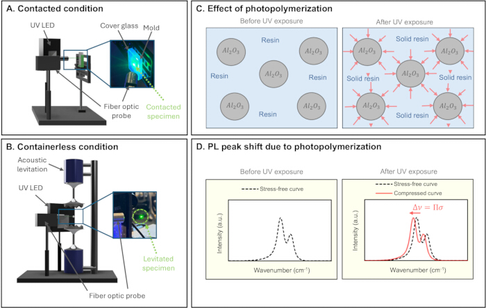
Figure 1. PL setup and measurement principle for contacted and containerless curing. (A) Contacted condition with the resin placed in a mold under UV curing and PL collection. (B) Containerless condition with the resin bead suspended in the acoustic levitation field during UV curing and PL collection. (C) Photopolymerization solidifies the resin around alumina particles and generates local compressive stress. (D) The transferred compressive stress shifts the alumina photoluminescence peak relative to the initial stress-free position. Please click here to view a larger version of this figure.

The Cr³⁺ ions substitute for aluminum ions within the trigonal crystal structure of α-alumina, making the luminescence response sensitive to changes in the local stress state¹¹. Under applied or residual stress, the R-line peak positions shift relative to their stress-free positions. This stress-dependent shift is known as the piezospectroscopic effect, and it provides a direct method for relating measured peak shifts to local stress around alumina particles.

Synchrotron X-ray diffraction provides a complementary method for evaluating residual strain and stress in alumina-containing materials. XRD has been widely used to study residual stresses in alumina ceramics^12,13,14 and enables non-destructive measurement of lattice spacing changes in crystalline materials¹⁵. In this study, the diffraction response of alumina particles was used to track changes in lattice spacing during curing. These lattice spacing changes can be related to strain and, with appropriate elastic constants, to stress.

Having established alumina as the model system, the choice to couple two independent characterization techniques warrants explanation. Both PL and XRD offer independent stress and strain information in alumina-containing systems, but the combination of both techniques in this study offers advantages that cannot be achieved by either technique alone. PL can monitor the optical luminescence response of alumina at the particle level with high temporal resolution and is well-suited to follow the rapid stress evolution during the early phases of UV curing. XRD offers crystallographic validation of the PL results by independently probing the same underlying stress state through changes in alumina lattice spacing. Since the two measurements are made on the same material system and under the same contacted and containerless curing conditions, agreement between the two data sets further increases confidence in the observed peak-shift trends as indicators of residual stress. The combination of the two techniques provides a more complete and reliable picture of stress development due to curing in alumina-filled photopolymer nanocomposites than either method could provide alone.

Additionally, from a practical perspective, synchrotron XRD requires large-scale facility infrastructure that is not available in a space environment, and thus, is not suitable for in situ monitoring during actual in-space manufacturing operations. On the other hand, PL is a compact, portable, and fieldable technique that could be realistically used on future long-duration space missions. This work is a validation of the PL measurements against synchrotron XRD results in this ground-based study, and it establishes the credibility of PL as a standalone stress-monitoring tool that might be the primary characterization method when XRD is not accessible, such as in manufacturing operations aboard a spacecraft or planetary outpost.

These techniques provide the means to detect stress evolution during curing; however, variations in nanocomposites' properties and performance when manufactured under microgravity conditions are not yet fully characterized. It is fundamental to understand how space conditions alter the curing of polymer nanocomposites since this directly affects property or performance changes when compared with nanocomposites cured in Earth’s ambient conditions. Investigating this provides insight into the design of structural and functional materials through in-space manufacturing^{16,17,18,19,20,21}.

It is clear that in-space and ground-based manufacturing differ in their environmental conditions. This motivates a unique, dependable, and accessible special ground-based setup to simulate the space conditions that are necessary to design and validate the properties and performance of materials manufactured in space. The conditions needed to simulate space environments are thermal cycles, vacuum, radiation, and microgravity. These affect the curing dynamics, microstructural evolution, as well as bonding and dispersion of the nanoparticles. Understanding these effects will enable progress and development towards reliable in-space manufacturing that will improve the safety and longevity of space missions while offering the relevant processing conditions for creating new material functionalities.

Acoustic levitation is a practical ground-based test method that is used to simulate processing in microgravity by facilitating a containerless environment. It is not equivalent to microgravity. The levitated object is supported by a nonuniform acoustic radiation force that counteracts gravity, rather than existing in a genuinely reduced-gravity environment. However, it removes the mechanical constraint imposed by a mold or container wall, which is the specific condition of interest for this study. This technique is commonly used in the field of materials science, chemistry, biology, bioengineering, and other sciences^{16,22,23,24,25,26,27}. Acoustic levitation generates acoustic radiation pressure produced by sound waves that enable an object to suspend in midair²³ and provide a containerless environment in which to investigate curing dynamics without container-induced mechanical constraint. The high temporal resolution offered by both spectroscopy and synchrotron X-ray diffraction makes them ideal techniques for studying the relatively short time frames associated with the photopolymer curing process. This work is particularly relevant to microgravity as it addresses a fundamental materials processing challenge for in-space manufacturing: how the absence of containers, a condition inherently present in microgravity, alters the residual stress state of a curing nanocomposite. The containerless condition studied here serves as a ground-based analog for microgravity processing, and the quantitative comparison of spectral changes reflecting stress development between contacted and containerless curing provides direct insight into how material properties may differ when the same nanocomposite system is manufactured in space versus on Earth. This paper details the methods that integrate acoustic levitation with powerful in situ spectroscopy and x-ray diffraction characterization to reveal the effects of containerless processing on the curing of a polymer nanoparticle system consisting of alumina nanoparticles and photopolymer.

Acoustic levitation has previously been combined with beamline techniques, including energy-dispersive X-ray diffraction to follow crystallization in levitated droplets²⁸, synchrotron SAXS of concentrated protein solutions²⁹, and as a sample-delivery platform for room-temperature macromolecular X-ray crystallography^30,31. However, these studies have focused on crystallization, structural characterization, or sample delivery rather than the time-resolved evolution of curing-induced lattice strain during polymerization. To the authors' knowledge, this study is the first to combine acoustic levitation with time-resolved in situ synchrotron XRD to track lattice strain evolution during an active photopolymerization reaction, alongside a directly comparable contacted condition to isolate the effect of container-wall constraint on curing-induced residual stress.

Based on the mechanical role of container-wall constraint in restricting volumetric shrinkage during curing, it is hypothesized that the presence or absence of this constraint will produce measurably different residual stress states in the cured nanocomposite, with the contacted condition expected to develop higher and more constrained residual stress than the containerless condition, where the specimen can shrink more freely in the absence of a solid boundary.

Protocol

Material selection

α-Alumina nanopowder was used as the ceramic filler. According to the manufacturer's specification, the powder has a grain size of approximately 40 nm, determined by X-ray line broadening, an average particle size (APS) of 150 nm, determined by BET specific surface area and SEM, and a BET multi-point specific surface area of approximately 10 m²/g. Based on previous studies of particle dispersion in filled photopolymer and epoxy systems³² very low alumina loadings (e.g., 5 vol%) were found to produce a weak photoluminescent response and poor particle dispersion, making them unsuitable for opto-mechanical stress sensing, while higher loadings (e.g., 20 vol%) produced a significant increase in viscosity that made the mixture difficult to inject and mix uniformly, despite providing a stronger signal. A concentration of 15 vol% alumina was therefore selected as a compromise between manufacturability, sensing performance, and dispersion quality.

Experimental Setup

Portable piezospectroscopy system (PPS) setup

The PL experiments utilized a previously developed Portable Piezospectroscopy (PPS) system consisting of an InPhotonics Inc. RPB Raman probe, a compact, two-way fiber-optic probe featuring a dichroic mirror and custom objective f/3 lens^33,34. The overall PPS system includes both hardware and software components. The hardware consists of a spectrograph, charge-coupled device (CCD), laser, fiber optics, and computer^33,34. For the software, two main programs are utilized: MATLAB and LightField. MATLAB-based programs are mainly used for data post-processing, and LightField is used to gather the data from the CCD. Figure 1 shows the complete experimental setup for both curing conditions alongside the underlying measurement principle, illustrating the contacted (mold) and containerless (acoustic levitation) configurations(Figure 1A and Figure 1B), the compressive stress generated in the alumina particles upon resin solidification (Figure 1C), and the corresponding photoluminescence peak shift used as an indicator of that stress (Figure 1D). In the container setup, the mold fixture was positioned at the same location as the center of the acoustic levitation field to maintain consistent geometry between the two configurations. The UV LED unit (405 nm wavelength, 10 W rated power, IP66-rated housing) was placed at a distance of 6 cm from the specimen, and the fiber-optic probe was directed at the specimen to collect the photoluminescence signal continuously during curing. The UV LED was positioned to avoid direct illumination of the fiber-optic probe, preventing fiber damage. Alumina photoluminescence peaks were collected over time during UV curing, and peak shifts were monitored as shown in Figure 1D. During photopolymerization, the resin solidifies around embedded alumina particles and undergoes polymerization shrinkage, generating local compressive stress that is transferred to the alumina particles (Figure 1C), causing the photoluminescence peak to shift from its initial stress-free position. Peak positions were then extracted from LightField, and the peak shift was calculated in MATLAB by comparing each peak position with the initial peak position before UV exposure.

Synchrotron X-ray diffraction setup

Synchrotron X-ray diffraction (XRD) measurements were performed in situ during the curing process on the 6-ID-D beamline of the Advanced Photon Source at Argonne National Laboratory, USA. Figure 2 presents the synchrotron XRD setup for both the contacted and containerless conditions, along with the measurement principle showing how curing-induced stress alters the alumina lattice spacing to produce a detectable peak shift (Figure 2A–C).

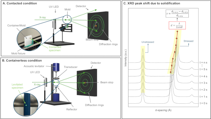
Figure 2. Synchrotron X-ray diffraction setup and measurement principle for contacted and containerless curing. (A) Contacted condition with the resin placed in a mold during UV curing and XRD collection. (B) Containerless condition with the resin bead suspended in the acoustic levitation field during UV curing and XRD collection. (C) Curing-induced stress changes the alumina lattice spacing, causing an XRD peak shift that is used to calculate strain during solidification. Please click here to view a larger version of this figure.

The specimen was irradiated with a parallel beam of 90.5 keV photons (corresponding to a wavelength of λ = 0.137 ˚A) with approximate dimensions of 0.5 × 0.5 mm, positioned approximately at the center of the specimen, as shown in Figure 2A,B. The sample-to-detector distance was set to approximately 1.5 m to capture the alumina peaks of interest. Ring-like diffraction patterns were recorded on a Varex XRD 4343RF flat-panel detector (2880 × 2880 pixel matrix, 150 µm pixel pitch) capable of high-speed real-time imaging at up to 15 fps. Data were collected for a total acquisition time of 600 s per experiment.

As with the PPS setup, measurements were performed under both contacted and containerless conditions (Figure 2A,B). The UV LED was placed 6 cm from the specimen, consistent with the PPS configuration, and the mold fixture and levitated specimen were positioned at the same measurement location to maintain geometric consistency. The full rig assembly was mounted on a linear stage to allow alignment of either the contacted specimen or levitated bead with the beamline as needed. XRD peak shifts were then monitored over time throughout UV curing (Figure 2C), as curing-induced stress transferred to the embedded alumina particles produces a measurable change in lattice spacing.

Sample preparation

Alumina powder was mixed at 15 vol% with liquid resin in a beaker/mixing container and stirred with a stirring rod to promote homogeneous dispersion of the alumina particles, as illustrated in Figure 3A.

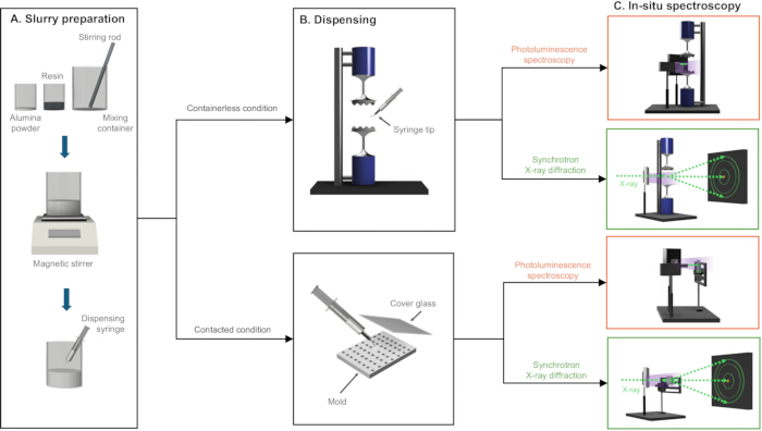
Figure 3. Sample preparation, dispensing, and in situ measurement workflow. (A) Alumina powder and liquid resin are mixed to prepare a homogeneous nanocomposite slurry. (B) The prepared slurry is dispensed into either the acoustic levitation field to form a containerless bead or into the silicone mold for the contacted condition. (C) PL and synchrotron XRD measurements are performed for both containerless and contacted curing conditions to compare spectral changes reflecting residual stress and structural evolution. Please click here to view a larger version of this figure.

The nanocomposite slurry formulation was maintained on a magnetic stirrer throughout the experiment to keep the alumina particles well dispersed. Once dispersed, the slurry was loaded into a dispensing syringe in preparation for specimen delivery, as shown in Figure 3A. Prior to each experiment, the prepared slurry was loaded into a syringe for dispensing into either the acoustic levitation field or the silicone mold.

Sample dispensing and controlled levitation

For the acoustic levitation (containerless) condition, the acoustic node region was located prior to dispensing. The loaded syringe was held at approximately 45° relative to the ground plane (Figure 3B), and the slurry was slowly injected into the levitator until a stable elliptical bead shape was achieved within the acoustic field, with an initial dispensed droplet volume of approximately 5–7 µL, adjusted as needed depending on the acoustic field conditions required to maintain a stable bead. After successful injection, the amplitude in the levitation software was adjusted to stabilize the bead.

Two different single-axis and dual-axis acoustic levitator configurations from the same manufacturer were used, depending on the measurement modality. Both configurations operated at an automatically calibrated resonant frequency of approximately 22,400–22,450 Hz upon activation, with the operating frequency fixed by the device's automatic calibration rather than manually set. For synchrotron XRD experiments at Argonne National Laboratory (ANL), a single-axis configuration was used, consisting of one ultrasonic transducer positioned above one reflector, with the transducer-reflector spacing fixed according to the levitator’s standard manufacturer setup. For PPS experiments, a dual-axis configuration was used, consisting of two opposing ultrasonic transducers (top and bottom), with transducer spacing likewise fixed per the manufacturer’s standard setup.

In both configurations, the acoustic node location and the specimen position within the field were kept consistent across replicate specimens within a session: the position of the first dispensed specimen was set using the alignment laser guide, and subsequent specimens were dispensed at that same reference position, so that beam and probe focus did not need to be re-established for each new specimen.

For the XRD single-axis system, the amplitude was increased until the acoustic tone emitted by the levitator was audible, at which point the slurry was injected via syringe into the node. The amplitude was then adjusted to support stable levitation.

For the PPS dual-axis system, the top and bottom transducer amplitudes were adjusted independently through the software until the bead was stably trapped and were not actively readjusted for the remainder of a given curing run.

In both configurations, the levitation condition was considered acceptable when bead motion about the node did not displace the specimen out of focus of the measurement beam: for XRD, the bead was required to remain aligned within the ~500 µm X-ray beam footprint at the measurement location (see Synchrotron X-ray Diffraction Setup); for PPS, the bead was required to remain within the focal spot of the fiber-optic probe, confirmed by continued detection of a clear, well-defined alumina photoluminescence peak on the live acquisition software.

For the contacted (silicone mold) condition, the slurry was dispensed directly into the mold using the loaded syringe, also illustrated in Figure 3B. The mold cavity measured 3 × 3 × 2 mm, and the slurry was dispensed to fully fill the mold volume (~10.5 μL). Excess slurry was removed from the mold surface, and the mold was covered with a glass cover. PL and XRD experiments were then performed for both containerless and contacted conditions, as shown in Figure 3C. Each experiment was repeated to ensure comparability and reproducibility.

In situ data collection

Photoluminescence spectroscopy

After the specimen was placed in either the acoustic levitation field or the mold, the laser was powered on; protective glasses were worn throughout all laser operations. The focal point was optimized using LightField software to identify the strongest signal, confirmed visually as the smallest and brightest laser spot on the specimen. Alumina photoluminescence peak collection began prior to UV exposure, with peaks acquired every 0.5 s. After 5 s of pre-UV baseline collection, the UV LED was activated, and data collection continued for 5 min to ensure complete curing of the specimen. Following curing, the UV LED was turned off. For the containerless condition, the cured bead was retrieved into a container; for the contacted condition, the cured specimen was removed from the silicone mold using tweezers. Direct contact with the specimens was avoided throughout to prevent contamination and skin irritation.

Synchrotron X-ray diffraction

After specimen placement, the X-ray beam was aligned with the center of the specimen: the center of the levitated bead for the containerless condition and the center of the specimen inside the mold for the contacted condition. The experimental hutch was closed before the X-ray beam was activated. The X-ray beam and UV LED were turned on simultaneously, and diffraction data were collected throughout UV curing. Data collection continued until the specimen was fully cured; in this study, data were collected for 10 min to capture the full range of interest. After curing, the UV LED and X-ray beam were turned off, and specimens were collected as described for the spectroscopy setup, avoiding direct contact to prevent contamination and skin irritation.

Data Analysis

Photoluminescence peak fitting method

Raw photoluminescence spectra containing the alumina R1 and R2 peaks (Figure 4A) were extracted from the full curing dataset and imported into MATLAB for post-processing.

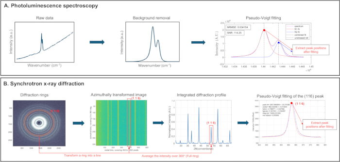
Figure 4. Data analysis workflow for PL and synchrotron XRD measurements. (A) PL spectra are processed by background removal and pseudo-Voigt fitting of the alumina R1 and R2 peaks to extract peak positions during curing. (B) Synchrotron XRD diffraction rings are transformed and integrated into a one-dimensional diffraction profile, followed by pseudo-Voigt fitting of the alumina (116) peak to extract the peak position and calculate curing-induced strain. Please click here to view a larger version of this figure.

Background noise was removed from each spectrum, and the slanted baseline was corrected to approximately align with the x-axis. Pseudo-Voigt fitting was applied to the alumina photoluminescence peaks to accurately fit the R1 and R2 peaks³⁵. Peaks were fit using a constrained nonlinear optimization algorithm (fmincon) to a pseudo-Voigt function, with area, center position, FWHM, and a shape factor (0 = pure Gaussian, 1 = pure Lorentzian) as the four free parameters per peak (R1 and R2). A linear background, fit to the raw intensity at 14300 and 14500 cm⁻¹, was subtracted from each spectrum prior to fitting. Initial parameter guesses were estimated directly from each smoothed, baseline-corrected spectrum, and fit bounds were set as a percentage range around each initial guess (area: 50–150%; FWHM: 60–180%). Fit quality was assessed using the normalized root-mean-square error (NRMSE). Fitted peak positions were extracted at each time point throughout the curing process, and peak shifts were calculated by comparing each fitted position to the initial pre-UV-exposure value.

XRD peak fitting method

Two-dimensional diffraction images were imported into the XRD processing software or MATLAB for analysis. XRD data can be analyzed to yield information on material strain^36,37,38. Diffraction rings from the alumina particles were identified (Figure 4B), and the ring corresponding to the alumina (116) peak was selected based on its clarity for tracking lattice spacing changes. Identifying the rings directly in the 2D diffraction image at this stage served as a qualitative check of data quality prior to integration, confirming complete and continuous rings (indicating uniform specimen illumination and absence of beam clipping), correct detector alignment and center position, and the absence of parasitic scattering or spurious features that could distort the integrated profile. Once ring quality was confirmed, the selected ring was transformed into an azimuthally transformed image and integrated over the full 360° azimuthal range to yield a one-dimensional diffraction profile, which was then used for quantitative peak-position fitting to extract d-spacing and calculate curing-induced strain. The alumina (116) peak in the integrated profile was fitted with a pseudo-Voigt function to determine the peak position, and was then extracted at each diffraction frame during curing. Peaks were fit using a nonlinear least-squares algorithm (lsqnonlin) to a pseudo-Voigt function, with intensity, center position, width (FWHM), and shape (Gaussian-to-Lorentzian ratio) as fit parameters. A linear background was subtracted from each spectrum before fitting. Fits were bound-constrained with a convergence tolerance of 10⁻⁴. The change in lattice spacing was calculated from the fitted peak positions using Bragg’s law:

where d is the lattice spacing, n is the diffraction order, λ is the x-ray wavelength, and θ is the Bragg angle. For direct comparison with standard alumina reference diffraction patterns, which are conventionally indexed using Cu Ka radiation, the measured d-spacings were additionally used to calculate an equivalent 2θ value corresponding to Cu Ka radiation λ = 1.54056 Å via Bragg's law. This conventional equivalent 2θ scale, rather than the native synchrotron 2θ scale (λ = 0.137 Å), is used for the diffraction angle axis. Curing-induced strain was then calculated by comparing the lattice spacing at each time point with the initial value before UV exposure:

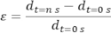
where d_{t = n s} is the lattice spacing at each time point during curing and d₀ is the initial lattice spacing before UV exposure.

Results

Photoluminescence spectroscopy results

The early-stage PL response provides insight into how curing-induced stress develops under contacted and containerless conditions. Figure 5 shows the mean evolution of the alumina photoluminescence peak position over the first 20 s for both conditions, capturing the pre-UV baseline, the rapid wavenumber decrease that occurs immediately after UV exposure, and the subsequent partial recovery as curing progresses.

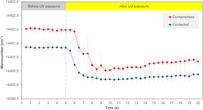
Figure 5. Average PL results showing early-stage wavenumber evolution during UV curing. The alumina photoluminescence peak position was averaged across three replicate specimens (n = 3) per condition and tracked for the first 20 s of curing under contacted and containerless conditions. Error bars represent the standard deviation among specimens. The first 5 s represents the pre-UV baseline, followed by UV exposure, a rapid curing-induced wavenumber decrease due to compressive stress transfer from the solidifying resin to the embedded alumina particles, and a subsequent partial recovery as the polymer network stabilizes. Please click here to view a larger version of this figure.

For PL, three independent specimens (n = 3) were measured per condition. Raw data for all three replicates per condition are provided in the data availability statement.

The first 20 s of curing is especially important because the largest wavenumber change occurs during this period, indicating that the most rapid stress evolution happens shortly after UV exposure begins. Before UV exposure, the two conditions show different initial wavenumbers. This pre-UV difference between conditions is 0.660 cm^-1 (mean initial wavenumber of 14402.01 ± 0.028 cm^-1 for containerless and 14401.350 ± 0.009 cm^-1 for contacted, n = 3). All subsequent peak-shift values reported in this study are calculated relative to each specimen's own pre-UV baseline.

After the UV LED is turned on at 5 s, the resin rapidly photopolymerizes and starts to solidify around the embedded alumina particles, and the alumina peak correspondingly shifts to a lower wavenumber. The surface-contacted specimen shows a faster decrease in wavenumber between approximately 5 and 7 s. In contrast, the containerless specimen shows a more gradual decrease, suggesting slower stress development without mold-wall constraint.

Following this rapid decrease, both conditions reach a minimum mean wavenumber and subsequently show a partial recovery toward higher wavenumber as curing continues. The contacted condition reaches its minimum earlier and shows a smaller, more gradual recovery, remaining relatively stable through the remainder of the 20 s window. The containerless condition reaches its minimum slightly later and shows a more pronounced recovery beginning around 14 s.

All PL measurements met the criteria for a successful acquisition: a clear, well-resolved R1/R2 doublet with a high signal-to-noise ratio throughout the acquisition, and continuous specimen alignment within the fiber-optic probe's focal spot for the full curing duration. No specimens were excluded from the reported dataset. A suboptimal outcome, characterized by partial loss of signal from bead drift outside the probe's focal spot or a distorted baseline requiring additional background correction, was not observed in this study but is noted here to support reproducibility.

Containerless specimen morphology during controlled levitation

The early-stage image sequence of the containerless specimen helps explain how the levitated resin bead physically responds during UV curing. Figure 6 shows the bead morphology at successive time points from the liquid state through gelation and rapid solidification, capturing the full shape evolution from UV activation to the stable solid state at 60 s, with a final bead size of 2.5 × 2.5 × 1.4 mm.

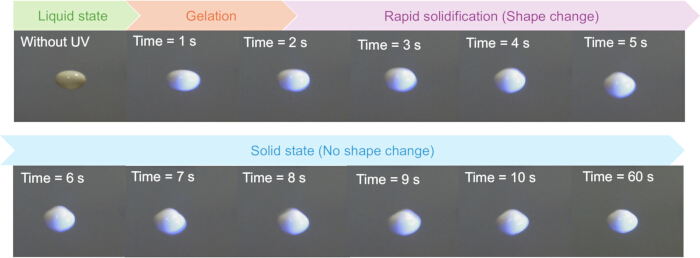
Figure 6: Representative shape evolution of a levitated resin bead during UV curing. The bead remains liquid before UV exposure, gels at approximately 1 s, undergoes visible shape change during rapid solidification between 2–5 s, and reaches a stable solid state by 6 s with no further change through 60 s. Final cured bead size: 2.5 × 2.5 × 1.4 mm. Please click here to view a larger version of this figure.

Before UV exposure, since the bead is liquid, it remains smooth and rounded while levitated in the acoustic field. After the UV LED is activated, the bead begins to gel within the first 1–2 s. Between 3 and 5 s, the bead changes shape more clearly. It becomes slightly distorted and less smooth. After about 6 s, the bead is mostly solid, and the shape does not change much. From 6 to 60 s, the bead stays relatively stable, showing that the main curing and shape change happen in the first few seconds after UV exposure.

A successful containerless run was characterized by a bead that remained within the acoustic node and imaging field throughout gelation and solidification, allowing morphology to be captured at every time point. Some bead movement and shifting during curing is expected, as the change in mass distribution and surface properties during gelation and solidification alters the mechanical response to the acoustic field. A suboptimal outcome, involving movement or drift severe enough to displace the bead out of the imaging frame or acoustic node entirely, was not observed in this study but is noted here to support reproducibility.

Synchrotron X-ray diffraction results

The diffraction profiles compare pure alumina powder with the 10 min cured specimens from the surface-contacted and containerless curing conditions. Figure 7 presents the full diffraction profiles for all three specimens alongside a zoomed view of the (116) peak, where the shift in 2θ position directly reflects the magnitude of curing-induced lattice strain in each condition.

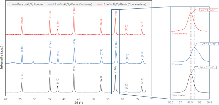
Figure 7. Representative XRD peak shift after UV curing. XRD profiles of pure alumina powder and 10 min cured contacted and containerless specimens are compared, with the diffraction angle axis presented as an equivalent conventional angle scale for comparison with standard alumina reference patterns, rather than the native synchrotron scale. The zoomed alumina peak shows the largest shift for the contacted specimen, consistent with higher curing-induced residual stress. Please click here to view a larger version of this figure.

The alumina (116) peak was selected for peak-shift analysis because it provides a clear peak for tracking changes in lattice spacing. In the zoomed (116) region, the contacted specimen shows the largest peak shift compared with the pure alumina powder. The containerless specimen also shows a peak shift, but the shift is smaller than that of the contacted specimen. This trend agrees with the PL results, where the contacted condition showed a larger stress-related peak shift than the containerless condition. Therefore, both PL and XRD results support that the curing environment affects residual stress development in the alumina-filled photopolymer nanocomposite.

For XRD, three independent specimens (n = 3) were measured per condition. Raw data for all three replicates per condition are provided in the data availability statement. Figure 7 presents one representative specimen per condition; across the three replicates, the final (116) peak position averaged 57.523° ± 0.042° 2θ (conventional) for the containerless condition and 57.786° ± 0.152° 2θ (conventional) for the contacted condition, consistent with the representative trend shown in Figure 7.

A successful XRD run was characterized by a bead that remained within the X-ray beam footprint throughout curing, yielding complete, continuous diffraction rings suitable for azimuthal integration and peak fitting. A suboptimal outcome occurred when bead motion within the acoustic field displaced the specimen away from the beam footprint, resulting in incomplete or clipped diffraction rings.

DATA AVAILABILITY:

The dataset supporting the findings of this study has been deposited in the Zenodo repository and is publicly available at https://doi.org/10.5281/zenodo.20498417. The datasets uploaded have been acquired using two methods: photo-luminescence spectroscopy and synchrotron X-ray diffraction. Data was collected in situ with the curing of nanocomposites in an acoustic levitator.

Discussion

Pre-UV mechanical preloading in the contacted condition

The lower initial wavenumber observed in the contacted specimen (Figure 5) suggests that stress may already be introduced before curing, likely due to sample preparation, confinement by the mold, or interaction with the cover glass. Because the contacted specimen is enclosed by both the silicone mold and the cover glass prior to curing, while the containerless specimen is dispensed into the acoustic field without any solid contact, the lower initial wavenumber observed in the contacted condition is attributed to a compressive mechanical load applied to the specimen during mold and cover-glass enclosure. This offset is present before UV exposure begins and therefore reflects a mechanical preloading effect rather than a curing-related process. The pre-existing offset, therefore, does not affect the reported evolution of the peak position within each condition, but it does mean the two conditions begin curing from different absolute wavenumber states, which should be considered when comparing absolute wavenumber values between conditions rather than their time-dependent evolution.

Rate and recovery of stress evolution during curing

The contacted specimen has a faster wavenumber decrease between approximately 5 and 7 s (Figure 5), indicating more rapid stress buildup and resin hardening under the mold-constrained condition, whereas the containerless specimen has a more gradual decrease, suggesting slower stress development in the absence of container constraint. The subsequent partial recovery observed in both conditions is consistent with partial stress relaxation as the polymer network stabilizes. The contacted condition's earlier, smaller recovery and the containerless condition's later, more pronounced recovery are consistent with greater stress relaxation occurring in the absence of container constraint.

Bead morphology as evidence of curing kinetics

The bead morphology sequence (Figure 6) helps explain this behavior at the microstructural level. Before UV exposure, the bead remains in a liquid state. Gelation occurs at approximately 1 s, marking the point at which the resin begins to form a solid network. Between 2 and 5 s, the bead undergoes rapid solidification accompanied by visible shape change, as the resin hardens while the bead is still in motion within the acoustic field; once the resin becomes sufficiently solid, it can no longer relax back to its original rounded liquid shape, so some of this deformation becomes fixed. By approximately 6 s, the bead reaches a stable solid state with no further shape change through 60 s, indicating that the majority of curing-related shape change is confined to the first several seconds after UV exposure.

Confounding factors between curing conditions

While the higher residual stress observed in the contacted condition is consistent with the presence of a rigid wall constraint absent in the containerless condition, other factors distinguish the two curing environments and were not independently isolated in this study. UV wavelength and UV LED-to-specimen distance were held constant across both conditions, so these do not contribute to the observed difference. However, factors such as oxygen inhibition at exposed surfaces, specimen surface-area-to-volume ratio, heat transfer and dissipation, evaporative loss, specimen geometry, and curing kinetics could differ between the two conditions and were not independently separated in this work. Relatedly, the final bead shape differs somewhat between conditions: the contacted specimen is constrained to the disc-like geometry of the silicone mold, whereas the containerless specimen adopts an ellipsoidal shape shaped by the acoustic field. Because specimen geometry can itself influence local shrinkage gradients and curing behavior, this shape difference is a further factor that was not isolated in the present study. However, the two specimen types remain broadly comparable in overall size and are not drastically different in shape, and future work using matched or controlled specimen geometries across both conditions would help isolate this effect from that of wall constraint itself. Notably, these same factors are also inherent differences between Earth-based (mold-constrained) and in-space (containerless) manufacturing environments, rather than purely experimental artifacts to be eliminated. Isolating the individual contribution of each factor was outside the scope of the present study, which instead reports the net stress difference between the contacted and containerless curing environments as a whole.

It is worth noting that acoustic levitation reproduces a containerless mechanical boundary condition but does not fully replicate a true microgravity environment. The levitated bead's shape remained stable and reproducible across specimens (Figure 6), and no obvious particle settling was observed during curing, indicating that any internal flow generated by the acoustic field needed to stably levitate the specimen did not produce visible disruption to bead morphology or particle distribution. The consistency of the observed trend across replicate specimens, and across both PL and XRD, supports container-wall constraint as the primary driver of the differences observed between conditions.

The outcomes and findings presented here demonstrate the impact of these experimental techniques in providing accessible ground-based data showing the effects of containerless environments on the manufacturing of nanocomposites, prior to in-space missions for microgravity-assisted manufacturing. These results provide a basis for further optimizing manufacturing processes and material compositions for the development of functional materials for space applications.

The consistently larger peak shift observed in the contacted compared to the containerless condition, consistent with higher residual stress, has potential implications for in-space manufacturing. Materials processed in microgravity will naturally cure in a containerless state, so the residual stress built into the final part will differ from an identically formulated material manufactured on Earth in a mold. Residual stress is a known contributor to mechanical performance, dimensional stability, and long-term durability in cured polymer composites more broadly^39,40,41,42; however, the present study characterizes residual stress evolution only and does not include mechanical testing of the cured specimens. The extent to which the observed stress differences translate into measurable differences in mechanical performance or durability, therefore, remains to be established. These results nonetheless emphasize the need to consider the processing environment when qualifying nanocomposite materials for space applications, and suggest that Earth-based material property databases based on mold-cured specimens may not fully capture the residual stress state of the same material manufactured under containerless, microgravity-relevant conditions. Direct mechanical characterization of specimens cured under both conditions is an important direction for future work to establish this link.

Critical steps and troubleshooting

Two aspects of the containerless specimen preparation warrant particular attention for reproducibility. First, maintaining stable bead levitation during dispensing is sensitive to acoustic amplitude: if the bead displaces significantly about the acoustic node, this indicates the trapping force is imbalanced relative to the bead's mass and position. In this situation, amplitude should be decreased incrementally rather than in large steps, since reducing it below the level required for force balance will cause the bead to drop from the field. Amplitude adjustments are therefore best made in small increments while monitoring bead stability in real time, rather than as a single corrective step.

Second, reliable detachment of the slurry droplet from the syringe tip into the acoustic node is sensitive to several interacting factors, including slurry viscosity, surface tension, tip diameter, wetting behavior, droplet volume, and trapping strength. In this study, droplets were separated from an 18-gauge syringe tip (1.26 in length) using the acoustic radiation force alone, without manual separation, which was reliable for the droplet volumes and slurry viscosity used here. Readers attempting this with a droplet size at or below the syringe-tip diameter, or with higher-viscosity slurries, may find that the droplet does not fully separate from the tip under acoustic pull alone. In such cases, reducing slurry viscosity or switching to a larger-bore tip is recommended to achieve reliable droplet loading.

Materials

List of materials used in this article

Name	Company	Catalog Number	Comments
Alpha Alumina Powder	Inframat Advanced Materials	26N-0802A	Alumina Powder
d-SAL	Materials Development, Inc. (MDI)	-	Acoustic Levitation
Elegoo ABS-Like Photopolymer Resin	ELEGOO	X004C0BJT	Resin
INTLLAB MS-500	INTLLAB	-	Magnetic Stirrer
LightField	Teledyne Princeton Instruments, Trenton, NJ, USA	https://www.teledynevisionsolutions.com/en-in/products/lightfield/?model=LF&vertical=tvs-princeton-instruments&segment=tvs
MATLAB	The MathWorks, Inc., Natick, MA, USA	https://www.mathworks.com/products/matlab.html

References

- Merancy N. et al. ESDMD-001: Moon to Mars architecture definition document | Revision C - 2025. National Aeronautics and Space Administration; Washington (DC); 2025 Dec. Report No.: NASA/TP-20250010956. Available from: http://www.sti.nasa.gov
- Denis G. et al. From new space to big space: How commercial space dream is becoming a reality. Acta Astronaut. 2020;166:431—443.
- Mueller RP. Lunar base construction planning [conference presentation]. Presented at: Earth and Space 2022. 2022:858–870.
- Duke MB, Mendell WW. Scientific investigations at a lunar base. Acta Astronaut. 1988;17(7):675—690.
- Wahl McDonnell Douglas Corp BW, Wahl McDonnell BW. Analysis of selected opportunities for manufacturing in space. Vol. 2. 1969. Available from: https://commons.erau.edu/space-congress-proceedings/proceedings-1969-6th-v2/session-11/2
- Naser MZ, Chehab AI. Polymers in space exploration and commercialization. In: AlMaadeed MAA, Ponnamma D, Carignano MA, eds. Polymer Science and Innovative Applications. Elsevier; 2020:457—484.
- Dmitriev RI. et al. Versatile conjugated polymer nanoparticles for high-resolution O2 imaging in cells and 3D tissue models. ACS Nano. 2015;9(5):5275—5288.
- Li X. et al. High-temperature capacitive energy storage in polymer nanocomposites through nanoconfinement. Nat Commun. 2024;15(1):6655.
- Amberkar T, Mahanwar P. Phase change material nanocomposites for thermal energy storage applications. Materials Proceedings. 2022;9(1):8.
- Harsch M, Karger-Kocsis J, Holst M. Influence of fillers and additives on the cure kinetics of an epoxy/anhydride resin. Eur Polym J. 2007;43(4):1168—1178.
- Stevenson A, Jones A, Raghavan S. Stress-sensing nanomaterial calibrated with photostimulated luminescence emission. Nano Lett. 2011;11(8):3274—3278.
- Sarioglu C, Schumann E, Blachere JR, Pettit FS, Meier GH. X-ray determination of stresses in alumina scales on high temperature alloys. Materials at High Temperatures. 2000;17(1):109—115.
- Leoni M, Scardi P, Sglavo VM. Relaxation of indentation residual stress in alumina: Experimental observation by X-ray diffraction. J Eur Ceram Soc. 1998;18(12):1663—1668.
- Abuhasan A, Balasingh C, Predecki P. Residual stresses in Alumina/Silicon Carbide (Whisker) composites by X-ray diffraction. J Am Ceram Soc. 1990;73(8):2474—2484.
- Noyan IC, Cohen JB. Residual Stress: Measurement by Diffraction and Interpretation. Springer; 2013.
- Jantananont P, et al. Characterizing UV resin curing with additives under simulated microgravity for in-space manufacturing. Presented at: AIAA SciTech 2026 Forum; 2026 Jan 8. doi:10.2514/6.2026-1047.
- de Hoffmann SI, Greenwood LJ, Raghavan S. The use of regolith simulant as a material for building functional sensors in extreme environments. Presented at: Regional Student Conferences, 2025; 2025. doi:10.2514/6.2025-99380.
- Sorgi Johann ML, et al. Investigating the Raman characteristics of regolith simulants towards the creation of functional materials. Presented at: AIAA SCITECH 2025 Forum; 2025:2501.
- Astacio J, et al. In-space manufacturing of functional sensors. Presented at: 75th International Astronautical Congress (IAC 2024), 2024 IAF Microgravity Sciences and Processes Symposium; Milan, Italy; 2024:538–544.
- Warren P, et al. Effect of sintering temperature on microstructure and mechanical properties of molded Martian and Lunar regolith. Ceram Int. 2022;48(23):35825—35833.
- Latorre P, et al., inventors; University of Central Florida Research Foundation, Inc., assignee. Manufacturing sensors using celestial body regolith. United States patent US 12,576,583 B2. 2026 Mar 17.
- Tuckermann R, et al. Chemical analysis of acoustically levitated drops by Raman spectroscopy. Anal Bioanal Chem. 2009;394(5):1433—1441.
- Li L, Gu N, Dong H, Li B, Kenneth TVG. Analysis of the effects of acoustic levitation to simulate the microgravity environment on the development of early zebrafish embryos. RSC Adv. 2020;10(72):44593—44600.
- Boudreaux T, et al. Biological acoustic levitation and its potential application for microgravity study. Bioengineering. 2025;12(5).
- Vashi A, Yadav AS, Nguyen NT, Sreejith KR. Parametric analysis of acoustically levitated droplet for potential microgravity application. Appl Acoust. 2023;213.
- Wilke SK, et al. Microgravity effects on nonequilibrium melt processing of neodymium titanate: Thermophysical properties, atomic structure, glass formation and crystallization. npj Microgravity. 2024;10(1):26.
- Bauser HC, et al. A study on the stability of ritonavir form III processed in orbit and returned to Earth. npj Microgravity. 2026;12(1).
- Leiterer J, et al. The use of an acoustic levitator to follow crystallization in small droplets by energy-dispersive X-ray diffraction. J Appl Crystallogr. 2006;39(5):771—773.
- Sønderby P, et al. Concentrated protein solutions investigated using acoustic levitation and small-angle X-ray scattering. J Synchrotron Radiat. 2020;27(2):396—404.
- Tsujino S, Tomizaki T. Ultrasonic acoustic levitation for fast frame rate X-ray protein crystallography at room temperature. Sci Rep. 2016;6(1):25558.
- Morris RH, et al. Non-contact universal sample presentation for room temperature macromolecular crystallography using acoustic levitation. Sci Rep. 2019;9(1):12431.
- Andrade MAB, Marzo A, Adamowski JC. Acoustic levitation in mid-air: Recent advances, challenges, and future perspectives. Appl Phys Lett. 2020;116(25):250501.
- Hanhan I, Durnberg E, Freihofer G, Akin P, Raghavan S. Portable piezospectroscopy system: Non-contact in situ stress sensing through high resolution photo-luminescent mapping. J Instrum. 2014;9(11):P11005—P11005.
- Freihofer G, Poliah L, Walker K, Medina A, Raghavan S. Optical stress probe: In situ stress mapping with Raman and photo-stimulated luminescence spectroscopy. J Instrum. 2010;5(12):P12003—P12003.
- Raghavan S, Imbrie PK, Crossley WA. Spectral analysis of R-lines and vibronic sidebands in the emission spectrum of ruby using genetic algorithms. Appl Spectrosc. 2008;62(7):759—765.
- Rossmann L, et al. Method for conducting in situ high-temperature digital image correlation with simultaneous synchrotron measurements under thermomechanical conditions. Rev Sci Instrum. 2020;91(3):033705.
- Siddiqui SF, et al. Synchrotron X-ray measurement techniques for thermal barrier coated cylindrical samples under thermal gradients. Rev Sci Instrum. 2013;84(8):083904.
- Raghavan S, Imbrie P. High-resolution stress mapping of polycrystalline alumina compression using synchrotron X-ray diffraction. J Synchrotron Radiat. 2011;18(3):497—505.
- Shokrieh MM, Ghanei Mohammadi AR. The importance of measuring residual stresses in composite materials. In: Shokrieh MM, ed. Residual Stresses in Composite Materials. Woodhead Publishing; 2014:3—14.
- Shokrieh MM, Akbari S, Daneshvar A. Reduction of residual stresses in polymer composites using nano-additives. In: Shokrieh MM, ed. Residual Stresses in Composite Materials. Woodhead Publishing; 2014:246—268.
- Nardi T, et al. Stress reduction mechanisms during photopolymerization of functionally graded polymer nanocomposite coatings. Prog Org Coat. 2015;87:204—212.
- Rahimian-Koloor SM, Shokrieh MM. Investigating the effect of the curing-induced residual stress on the mechanical behavior of carbon nanotube/epoxy nanocomposites by molecular dynamics simulation. Eng Sci. 2023;22:817.
Reprints and Permissions
This article has been published
Video Coming Soon