This study investigates electroencephalography biomarkers for distinguishing Alzheimer’s disease, frontotemporal dementia, and healthy controls. Random Forest models using root mean square, power spectral density, and entropy features were interpreted using explainable artificial intelligence and effect-size analysis. Removing low-impact entropy features improved classification performance, achieving 94% test accuracy.
Research Article
Multidomain Electroencephalography Biomarker Fusion for Machine Learning-Based Dementia Classification
In This Article
Summary
Abstract
Electroencephalography (EEG) has been investigated as a noninvasive approach for characterizing brain activity in neurodegenerative conditions. This study evaluated whether multidomain EEG biomarkers could distinguish Alzheimer’s disease (AD), frontotemporal dementia (FTD), and healthy controls (HC). The publicly available dataset contained resting-state, eyes-closed EEG recordings from 88 participants, including 36 with AD, 23 with FTD, and 29 healthy controls. Multidomain EEG biomarkers and demographic features were extracted for machine learning classification. The EEG-derived features included root-mean-square (RMS), power spectral density (PSD), and entropy measures. A Random Forest classifier was trained using the combined feature set and interpreted using explainable artificial intelligence. Feature-stability and Cohen’s d effect-size analyses were performed to evaluate feature contributions, followed by an ablation analysis. Entropy-based features showed the lowest contribution to classification. The complete multidomain model achieved 96% training accuracy and 92% test accuracy. After the removal of the entropy features, test accuracy increased to 94%. These results describe the classification performance of the selected multidomain EEG and demographic features within the Random Forest framework.
Introduction
Alzheimer’s disease (AD) is a progressive neurological condition associated with deterioration in cognitive and motor function. Its prevalence increases substantially with age, and dementia is a major cause of morbidity and mortality among older adults1,2,3,4,5. Because diagnosis and disease classification remain challenging, analysis of brain signals has been investigated as a means of characterizing neurophysiological changes associated with dementia.
Electroencephalography (EEG) is a noninvasive method for recording the electrical activity of the brain and has been investigated in Alzheimer’s disease and other neurological disorders6,7,8,9,10,11. EEG signals reflect electrical potentials generated by neuronal activity and are recorded noninvasively from multiple scalp locations12,13,14. Brain activity is commonly characterized using delta, theta, alpha, beta, and gamma frequency bands15. Alzheimer’s disease has been associated with EEG slowing, reduced signal complexity, and altered synchronization16. Spectral analyses have reported increased delta and theta activity together with reduced alpha and beta activity in individuals with AD compared with healthy controls17,18,19. Previous EEG classification studies have reported high performance for distinguishing AD from healthy controls (HC) and frontotemporal dementia (FTD) from HC. In contrast, discrimination between AD and FTD has generally been more challenging10,11.
Machine learning methods have been used to identify patterns in EEG signals associated with neurological disease20,21. Feature extraction is therefore an important component of EEG-based classification. Previous studies have investigated spectral, temporal, complexity, and functional connectivity features in combination with machine learning models3,15,22,23. Spectral features are particularly relevant because they quantify frequency-dependent changes in brain activity, including reduced alpha activity and increased theta activity reported in AD23,24,25,26.
Several EEG-based studies have evaluated different combinations of features, classifiers, and validation strategies. Connectivity-based analysis has been used to distinguish AD, FTD, and HC, with reported classification performance varying depending on the comparison and feature-selection procedure27. Fourier-based features have also been evaluated for distinguishing AD, mild cognitive impairment (MCI), and healthy controls, although limitations included limited preprocessing and possible overfitting associated with the validation strategy28. Nonlinear EEG complexity measures have shown discriminative potential for AD classification, with some achieving high accuracy, sensitivity, and specificity, although their applicability to MCI and disease-stage discrimination remains limited21.
Deep learning methods based on time-frequency EEG representations have also been investigated for multiclass classification of AD, MCI, and HC29. Although high classification performance has been reported, limitations include small or selected cohorts, class imbalance, heterogeneous disease severity, lack of external validation, and reduced model interpretability29. Validation strategy is also an important methodological consideration. Participant-independent approaches have demonstrated that conventional epoch-level cross-validation may overestimate performance when epochs from the same participant appear in both training and testing sets30. This limitation is particularly relevant when comparing classification results across studies that use different validation schemes.
Complexity and connectivity measures have also been evaluated using support vector machine classifiers, with phase-based connectivity and multiscale entropy showing varying levels of discriminative performance31,32. Other work using Fourier- and wavelet-derived features has reported variable performance across AD, MCI, and HC comparisons, with multiclass classification generally remaining more difficult than binary classification14. Entropy- and synchrony-based approaches have additionally demonstrated discrimination between AD and control groups, although the characteristics of the control population may affect the observed effect size2.
The present study evaluates a multidomain feature set comprising root-mean-square (RMS), power spectral density (PSD), and entropy measures extracted from EEG frequency bands, along with age as a demographic variable. RMS represents signal amplitude within each frequency band, whereas PSD represents frequency-domain power. Entropy is included as a measure of signal complexity. These features provide complementary descriptions of EEG activity and are evaluated using a Random Forest classifier. The study further examines feature importance, feature stability, explainable artificial intelligence, and effect-size analysis to assess the relative contribution of the extracted features. The present study investigates the effectiveness of multidomain EEG features, including spectral, temporal, and complexity-based measures, in distinguishing Alzheimer’s disease (AD), frontotemporal dementia (FTD), and healthy controls (HC) using machine learning. It also examines which EEG frequency-band features contribute most strongly to classification when using power spectral density (PSD), root-mean-square (RMS), and entropy measures. In addition, the study compares the contributions of power-based features, including PSD and RMS, with those of entropy-based features and evaluates the contribution of age to the classification model.
Protocol
A schematic overview of the EEG preprocessing, feature extraction, and classification workflow is shown in Figure 1. The materials and software used in the study are listed in the Table of Materials.
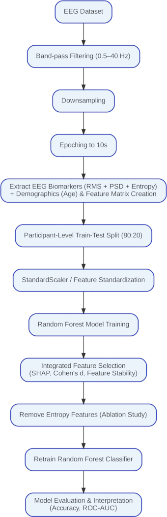
Figure 1: Workflow of the EEG preprocessing, feature extraction, and classification pipeline. Schematic overview of the study workflow, including EEG data verification, band-pass filtering and re-referencing, extraction of root mean square (RMS), power spectral density (PSD), and entropy features, addition of age, train-test splitting, Random Forest model development, feature-stability analysis, SHAP analysis, Cohen’s d effect-size analysis, integrated feature selection, entropy-feature ablation, model retraining, and performance evaluation. Please click here to view a larger version of this figure.
1. Data acquisition
The publicly available resting-state EEG dataset was obtained from the OpenNeuro repository (dataset ds004504, version 1.0.9)33. Participant labels and demographic information were verified. The dataset comprised 88 participants, including 36 participants with Alzheimer’s disease (AD), 23 with frontotemporal dementia (FTD), and 29 healthy controls (HC).
2. EEG recording import
For each participant, the EEG recording was loaded using the MNE-Python library. Each EEG file was checked to confirm that it was accessible, could be successfully imported, and contained a valid participant identifier. Recordings with missing or corrupted files were excluded. The original EEG sampling frequency of 500 Hz was retained at this stage. The signals were downsampled to reduce computational load while preserving all clinically relevant EEG information for this study.
3. Band-pass filtering
The continuous EEG recordings were filtered using a fourth-order band-pass filter with a low cutoff frequency of 0.5 Hz and a high cutoff frequency of 40 Hz.
4. Common average referencing and epoching
Common average referencing (CAR) was applied to the filtered EEG recordings. At each time sample, the average signal across all available EEG channels was calculated and subtracted from each channel. The referenced EEG signals were retained for subsequent analysis. Each referenced EEG recording was segmented into fixed-length epochs using the make_fixed_length_epochs() function in MNE-Python. An epoch duration of 10 s with 0 s overlap was used.
5. Epoch validation
For each participant, only complete 10s epochs were retained. Any remaining EEG segment shorter than 10 s at the end of a recording was discarded. Each retained epoch was subsequently used as an individual sample for feature extraction.
6. Feature preparation
Although Mini-Mental State Examination (MMSE) data were available in the source dataset, they were excluded from the present analysis. The extracted EEG features were merged with participant demographic information, including age and diagnostic labels, obtained from the participants.csv metadata file. The participant identifier was used as the common key, and only participants with both EEG feature records and corresponding demographic information were retained.
The multidomain feature matrix included five root mean square (RMS) features (delta_rms, theta_rms, alpha_rms, beta_rms, and gamma_rms), five power spectral density (PSD) features (delta_psd, theta_psd, alpha_psd, beta_psd, and gamma_psd), and five entropy features (delta_entropy, theta_entropy, alpha_entropy, beta_entropy, and gamma_entropy). Age was included as a complementary demographic variable. Because age distributions may differ across diagnostic groups, demographic confounding could not be completely ruled out. Diagnostic group, defined as AD, HC, or FTD, was assigned as the target label.
7. Data preprocessing and train-test partitioning
During preprocessing, the recordings were downsampled from 500 Hz to 250 Hz to reduce computational requirements while retaining the EEG frequency information of interest.
The dataset was partitioned into training (80%) and testing (20%) subsets at the subject level using a grouped splitting strategy. Subject-level predictions were subsequently obtained by majority voting across the predicted epochs belonging to each participant. The primary evaluation used a subject-level grouped train-test split to prevent epochs from the same participant from appearing in both subsets. Subject-level predictions were obtained by majority voting across the predicted epochs belonging to each participant. The dataset was inspected for missing values, and missing observations were removed or imputed as applicable. Diagnostic labels were encoded. A StandardScaler was fitted on the training data and then applied to both the training and testing datasets.
8. Random forest model development
A Random Forest classifier was initialized using 80 trees, a maximum tree depth of 10, a maximum of four features, a minimum of five samples per leaf, and a random state of 42. The classifier was trained using the standardized training dataset.
9. Model evaluation
Class labels were predicted for both the training and testing datasets. A confusion matrix was constructed, and accuracy, precision, recall, and F1-score were calculated together with the classification report. Training and testing accuracies were recorded.
For the participant-wise evaluation, ensure that all epochs from a given participant were assigned exclusively to either the training or testing subset. The Random Forest classifier was trained using the same hyperparameters as in the primary analysis.
10. Cross-validation
As an additional model-evaluation procedure, five-fold stratified cross-validation was performed using shuffle = True and random_state = 30. The mean accuracy and standard deviation across the five folds were calculated. This analysis was considered separately from the primary subject-level holdout evaluation.
11. Feature-stability analysis
Feature stability was assessed by repeating Random Forest training 10 times using random seeds from 0 through 9. For each run, test accuracy and feature-importance scores were recorded. The mean and standard deviation of the feature-importance score for each predictor were calculated across the 10 runs, and the predictors were ranked according to their stability. This analysis was used to assess the consistency of feature rankings rather than to replace the primary subject-level evaluation.
12. Explainable artificial intelligence analysis
SHAP TreeExplainer was applied to the trained Random Forest model. SHAP values were calculated to estimate each feature's contribution to the model's predictions. The mean absolute SHAP value was calculated for each feature, and features were ranked according to their SHAP contributions. Features with consistently low SHAP values were identified and compared with the results of the feature-stability and Cohen’s d analyses. Features showing consistently low contributions were selected for subsequent ablation and model retraining.
13. Statistical effect-size analysis
Cohen’s d was calculated for each EEG biomarker for the AD versus HC, AD versus FTD, and FTD versus HC comparisons. Effect-size magnitudes were interpreted using thresholds of 0.20 for a small effect, 0.50 for a medium effect, and 0.80 for a large effect.
14. Integrated feature selection
The results of the Random Forest feature-importance analysis, SHAP analysis, and Cohen’s d analysis were compared. Predictors that consistently exhibited low feature importance, low SHAP contribution, and small effect sizes were identified as candidates for removal.
15. Feature ablation
Entropy features were evaluated in an exploratory ablation analysis, and a reduced feature matrix containing RMS, PSD, and age was constructed. The Random Forest classifier was retrained using the same hyperparameters. Model training, testing, cross-validation, and receiver operating characteristic (ROC) analysis were repeated using the reduced feature set.
16. ROC analysis
Class probabilities were obtained from the optimized Random Forest classifier. Multiclass ROC curves were generated using a one-versus-rest strategy. Class-specific area under the curve (AUC) values and the average AUC were calculated.
17. Performance comparison
The performance of the complete feature model was compared with that of the reduced feature model obtained after entropy-feature ablation.
Results
The Random Forest model achieved 96% training accuracy and 92% testing accuracy. The macro-average F1-score was 92%, while the weighted-average F1-score was also 92%, indicating comparable performance across the three classes, while the weighted-average F1-score was also 92%. Classification performance was highest for the Alzheimer’s disease (AD) class, whereas the frontotemporal dementia (FTD) class showed comparatively lower performance, as presented in Table 1.
Receiver operating characteristic (ROC) analysis was used to evaluate class separation across classification thresholds. As shown in Figure 2, the area under the ROC curve (AUC) exceeded 0.98 for all three classes, indicating high separability among the AD, FTD, and healthy control (HC) groups.
SHAP analysis using TreeExplainer was performed to evaluate feature contributions to the Random Forest classification model. The summary bar plot in Figure 3 showed the relative contribution of power spectral density (PSD), root mean square (RMS), entropy, and demographic features. Features with higher absolute SHAP values contributed more strongly to the model predictions, whereas entropy-related features showed comparatively low contributions.
Feature-stability analysis was performed by repeating Random Forest training across the specified random seeds. Test accuracy and feature-importance scores were recorded for each run, and the mean and standard deviation of feature importance were calculated. The model achieved 95% mean classification accuracy in this analysis, with a standard deviation of 0.17%. These repeated runs were used primarily to evaluate the consistency of feature rankings and were considered separately from the primary subject-level holdout evaluation. Age ranked highly in the feature-stability analysis, as shown in Table 2. The theta_psd and theta_rms features also ranked highly, whereas alpha_psd, alpha_rms, beta_psd, and beta_rms showed moderate feature importance.
Cohen’s d was calculated to assess the magnitude of group differences, as presented in Table 3. Alpha-band attenuation (alpha_rms, d = 0.97; alpha_psd, d = 0.87) and increased theta activity (theta_rms, d = 0.72) showed the largest reported differences between participants with AD and healthy controls. These findings were consistent with cortical slowing reported in EEG studies of dementia34. Entropy-based features showed comparatively smaller effect sizes. Comparisons between AD and FTD produced predominantly small-to-moderate effect sizes.
Alpha-band features showed large effect sizes for the AD-versus-HC and FTD-versus-HC comparisons. For AD versus HC, the reported effect sizes were −0.87 for alpha_psd and −0.97 for alpha_rms. For FTD versus HC, alpha-band attenuation was −0.73. The theta_psd feature showed an effect size of 0.61 for AD versus HC, while theta_rms showed an effect size of 0.72. Smaller differences were observed for AD versus FTD.
Beta-band features showed predominantly small-to-moderate group effect sizes. The beta_psd effect sizes were −0.35 for AD versus HC and −0.41 for AD versus FTD, while beta_rms showed mostly small effects. Gamma-band features showed moderate effects for some comparisons. The gamma_psd effect size was 0.47 for FTD versus HC and 0.20 for AD versus HC, while gamma_rms showed an effect size of 0.50 for FTD versus HC.
Delta PSD and RMS showed small positive effect sizes for AD versus HC (0.29 and 0.34, respectively) and FTD versus HC (0.25 and 0.25, respectively). Effect sizes for AD versus FTD were close to zero. Delta entropy showed small effect sizes across all three comparisons (0.08, 0.20, and −0.11).
Feature-stability, SHAP, and effect-size analyses indicated comparatively low contributions from the entropy features. Consequently, an ablation analysis was performed by excluding the entropy features and retaining RMS, PSD, and age. Following feature ablation, the Random Forest model achieved 96% training accuracy and 94% testing accuracy. This result was interpreted as an exploratory comparison within the evaluated feature-selection framework. Precision, recall, F1-score, and support for the AD, HC, and FTD classes are presented in Table 4.
Performance before and after entropy-feature ablation is compared in Table 5. Testing accuracy increased from 92% to 94% after removing entropy. Class-wise changes are presented in Table 6. For FTD, precision increased by 4%, and F1-score increased by 2%. Recall for the HC group increased by 4%, while precision decreased by 2%. Macro-average and weighted-average performance measures increased by approximately 1%–2% following feature ablation.
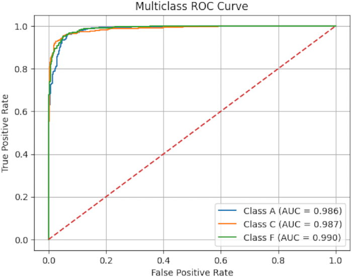
Figure 2: Receiver operating characteristic curves for Alzheimer’s disease, frontotemporal dementia, and healthy controls. Multiclass receiver operating characteristic (ROC) curves generated using the one-versus-rest strategy for Alzheimer’s disease (class A), frontotemporal dementia (class F), and healthy controls (class C). The area under the curve (AUC) was calculated for each class. Please click here to view a larger version of this figure.
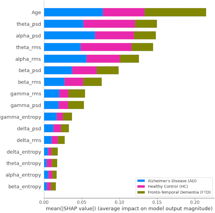
Figure 3: SHAP summary analysis of the trained Random Forest model. Summary bar plot showing the relative contribution of EEG-derived and demographic features to the Random Forest classification model. Mean absolute SHAP values were used to rank the contributions of root mean square (RMS), power spectral density (PSD), entropy, and age features. Please click here to view a larger version of this figure.
| Precision | Recall | F1-Score | Support | |
| Alzheimer’s | 0.92 | 0.95 | 0.94 | 579 |
| Control | 0.93 | 0.92 | 0.93 | 480 |
| Fronto Temporal Dementia | 0.93 | 0.87 | 0.9 | 314 |
| Macro average | 0.93 | 0.92 | 0.92 | 1373 |
| Weighted average | 0.93 | 0.92 | 0.92 | 1373 |
Table 1: Classification report on test data. Precision, recall, F1-score, and support for the Alzheimer’s disease, healthy control, and frontotemporal dementia classes in the test dataset, together with macro-average and weighted-average performance measures.
| Feature | Mean | Standard Deviation |
| Age | 0.1966 | 0.0017 |
| theta_psd | 0.0936 | 0.0027 |
| theta_rms | 0.0911 | 0.0023 |
| alpha_psd | 0.0824 | 0.0022 |
| alpha_rms | 0.0824 | 0.0024 |
| beta_psd | 0.0638 | 0.0013 |
| beta_rms | 0.0629 | 0.0012 |
| gamma_psd | 0.0534 | 0.001 |
| gamma_rms | 0.0527 | 0.0014 |
| delta_psd | 0.0403 | 0.0007 |
| delta_rms | 0.0359 | 0.001 |
| gamma_entropy | 0.0326 | 0.0008 |
| alpha_entropy | 0.0325 | 0.0006 |
| beta_entropy | 0.0283 | 0.0009 |
| theta_entropy | 0.0258 | 0.0004 |
| delta_entropy | 0.0255 | 0.0005 |
Table 2: Feature-stability ranking of the Random Forest model. Mean feature-importance values and corresponding variability obtained from repeated Random Forest training using random seeds from 0 – 9. Features were ranked according to their stability across runs.
| Feature | AD vs. HC | AD vs. FTD | FTD vs. HC |
| Delta PSD | 0.293 | -0.069 | 0.253 |
| Theta PSD | 0.612 | 0.23 | 0.355 |
| Alpha PSD | -0.869 | -0.219 | -0.64 |
| Beta PSD | -0.352 | -0.408 | 0.201 |
| Gamma PSD | 0.201 | -0.326 | 0.468 |
| Delta Entropy | 0.081 | 0.199 | -0.111 |
| Theta Entropy | 0.208 | 0.033 | 0.163 |
| Alpha Entropy | -0.061 | 0.071 | -0.137 |
| Beta Entropy | -0.37 | -0.042 | -0.332 |
| Gamma Entropy | -0.338 | 0.047 | -0.391 |
| Delta RMS | 0.342 | 0.041 | 0.251 |
| Theta RMS | 0.718 | 0.354 | 0.318 |
| Alpha RMS | -0.977 | -0.205 | -0.73 |
| Beta RMS | -0.494 | -0.365 | 0.015 |
| Gamma RMS | 0.187 | -0.33 | 0.5 |
Table 3: Cohen’s d effect-size comparison across diagnostic groups. Cohen’s d values for EEG biomarkers across the Alzheimer’s disease versus healthy control, Alzheimer’s disease versus frontotemporal dementia, and frontotemporal dementia versus healthy control comparisons.
| Precision | Recall | F1-Score | Support | |
| Alzheimer’s | 0.94 | 0.95 | 0.94 | 579 |
| Control | 0.91 | 0.96 | 0.94 | 480 |
| Fronto Temporal Dementia | 0.97 | 0.89 | 0.92 | 314 |
| Macro avg | 0.94 | 0.93 | 0.93 | 1373 |
| Weighted avg | 0.94 | 0.94 | 0.94 | 1373 |
Table 4: Classification report after feature ablation. Precision, recall, F1-score, and support for the Alzheimer’s disease, healthy control, and frontotemporal dementia classes after removal of entropy features and retraining of the Random Forest model.
| Metric | Before Ablation | After Ablation | Change |
| Training Accuracy | 0.96 | 0.96 | 0% change |
| Testing Accuracy | 0.92 | 0.94 | +2% improvement |
| Macro Precision | 0.93 | 0.94 | +1% improvement |
| Macro Recall | 0.92 | 0.93 | +1% improvement |
| Macro F1-Score | 0.92 | 0.93 | +1% improvement |
| Weighted Precision | 0.93 | 0.94 | +1% improvement |
| Weighted Recall | 0.92 | 0.94 | +2% improvement |
| Weighted F1-Score | 0.92 | 0.94 | +2% improvement |
Table 5: Performance comparison before and after feature ablation. Comparison of model performance metrics for the complete multidomain feature set and the reduced feature set obtained after removal of entropy features.
DATA AVAILABILITY:
The processed CSV dataset used for model development and analysis is provided as Supplementary File 1. The preprocessing code is available in a Python notebook at https://colab.research.google.com/drive/1PwidMZCbbIHdthDhat5OEZa7ya6f0-aC?usp=sharing, and the model-building and analysis code are available at https://colab.research.google.com/drive/1q8wYJjQpofAqZGYxz9xHKB0emGF4YGwM?usp=sharing. The processed CSV dataset can also be regenerated using the preprocessing code provided
| Class | Metric | Before | After | Change |
| Alzheimer’s | Precision | 0.92 | 0.94 | 0.02 |
| Recall | 0.95 | 0.95 | No change | |
| F1-score | 0.94 | 0.94 | No change | |
| Control | Precision | 0.93 | 0.91 | −2% |
| Recall | 0.92 | 0.96 | 0.04 | |
| F1-score | 0.93 | 0.94 | 0.01 | |
| FTD | Precision | 0.93 | 0.97 | 0.04 |
| Recall | 0.87 | 0.89 | 0.02 | |
| F1-score | 0.9 | 0.92 | 0.02 |
Table 6: Class-wise performance changes before and after feature ablation. Changes in precision, recall, and F1-score for the Alzheimer’s disease, healthy control, and frontotemporal dementia classes following the removal of entropy features.
Supplementary File 1: Processed epoch-level EEG feature dataset used for model development and analysis. Please click here to download this file.
Discussion
The Random Forest classifier was used to classify electroencephalography (EEG) samples into the Alzheimer’s disease (AD), frontotemporal dementia (FTD), and healthy control (HC) groups using multidomain features, including power spectral density (PSD), root mean square (RMS), and entropy measures. Age was included as a complementary demographic variable. Because age distributions could differ across diagnostic groups, demographic confounding could not be completely excluded, and the reported performance therefore reflected the combined contribution of demographic and electrophysiological information. The analysis examined the ability of multidomain EEG features to discriminate among AD, FTD, and HC groups and assessed the contribution of delta-, theta-, alpha-, beta-, and gamma-band features to classification35. Feature stability and effect size analyses indicated that power-based features, including PSD and RMS, contributed more strongly than entropy-based features. The extracted EEG biomarkers also reflected patterns associated with slowing of rhythms and reduced alpha activity.
Previous studies have evaluated entropy-, PSD-, and RMS-based EEG features using different machine learning approaches2,14,27,28,36,37. Entropy had been used to characterize EEG complexity and irregularity, while PSD had been used to quantify spectral characteristics2,14,27,28,36. RMS had also been evaluated as a frequency-band feature37. Using the same underlying dataset, previous work applied PSD-based binary classification with leave-one-subject-out validation33. The present analysis instead combined RMS, entropy, and PSD across the alpha, beta, gamma, theta, and delta bands within a multiclass classification framework. A lightweight EEG transformer was evaluated on the same dataset using a leave-one-subject-out binary classification strategy. A lightweight EEG transformer evaluated on the same dataset using a leave-one-subject-out binary classification strategy reported an accuracy of 83.28%. Direct numerical comparison with the present results should be interpreted cautiously because the classification task and validation procedures differed38.
Alpha-band features showed the largest effect sizes for differentiating AD from HC and FTD from HC, and increased theta activity also contributed to the differentiation of AD from HC. Beta-band features showed smaller effects across groups, whereas entropy-based features showed comparatively limited discriminative utility. Gamma-band features showed moderate effects for some comparisons, including FTD versus HC. Previous studies have reported lower alpha power and altered theta activity in AD and related diagnostic comparisons23,25,39. Entropy has also been described as a potentially informative biomarker in neurodegenerative disease36, indicating that its contribution may vary with the dataset, feature definition, and analytical approach.
Support vector machines had been used frequently in previous EEG classification studies3,21,24,37. The Random Forest classifier used in the present analysis provided feature-importance estimates and was applicable to the structured feature set used in this study40,41. Training and testing accuracies of 96% and 94%, respectively, were obtained after entropy-feature ablation. The removal of entropy features was associated with improved model performance, supporting the lower relative contribution observed for these features in the stability, SHAP, and effect-size analyses. Deep learning and transformer-based approaches have also been applied to EEG classification, although such approaches generally require larger datasets and are designed for higher-dimensional or sequential representations27,39,42,43,44,45.
EEG signals are noisy and non-stationary, and ensemble tree-based models can provide robustness when analysing structured feature representations. In the present study, RMS, PSD, entropy, and age were evaluated as complementary inputs to the Random Forest model. RMS represented signal amplitude within frequency bands, PSD represented spectral power, and entropy represented signal complexity. The findings indicated that PSD and RMS contributed more strongly than entropy to classification within the evaluated framework. Age also contributed to the model, although its inclusion introduced the possibility of demographic confounding. Future investigations could evaluate additional demographic variables and alternative machine learning or deep learning approaches in larger datasets to further assess generalisability and classification performance.
Disclosures
No known competing financial interests, personal relationships, financial relationships, or other activities that could have influenced the work reported in this study were declared.
Acknowledgements
The publicly available EEG dataset used in this study and the contributions of the researchers who made the dataset accessible for research purposes are acknowledged. No specific funding was received from public, commercial, or not-for-profit funding agencies.
Materials
| Name | Company | Catalog Number | Comments |
|---|---|---|---|
| Google Colab | [confirm environment]colab runtime | Cloud-based computational environment used to run the analysis notebooks | |
| MNE-Python | MNE-Python project | 1.12.1 | Used for EEG preprocessing, referencing, filtering, and epoch segmentation |
| NumPy | NumPy project | (2.0.2) | Used for numerical and array-based computations |
| OpenNeuro EEG dataset | OpenNeuro | ds004504, (1.0.9) | Publicly available resting-state EEG dataset containing AD, FTD, and HC recordings |
| Python | Python Software Foundation | [3.12.13 (main, Mar 4 2026, 09:23:07) [GCC 11.4.0]] | Programming environment used for data processing and model development |
| scikit-learn | scikit-learn project | 1.6.1 | Used for preprocessing, grouped data splitting, Random Forest classification, and performance evaluation |
| SciPy | SciPy project | (1.16.3) | Used for signal-processing and statistical computations |
| SHAP | SHAP project | 0.52.0 | Used for explainable artificial intelligence analysis with TreeExplainer |
References
- Rodrigues PM, et al. Early prediction of Alzheimer's with the electroencephalogram. Procedia Comput Sci. 2016;100:865–71. https://doi.org/10.1016/j.procs.2016.09.236
- Houmani N, et al. Diagnosis of Alzheimer's disease with electroencephalography in a differential framework. PLoS One. 2018;13(3):e0193607. https://doi.org/10.1371/journal.pone.0193607
- Tripanpitak K, et al. Biomarkers for Alzheimer's disease and mild cognitive impairment: recent advances in task-based EEG. J Alzheimers Dis. 2025 [Epub ahead of print].
- Kung HC, Hoyert DL, Xu J, Murphy SL. Deaths: final data for 2005. Natl Vital Stat Rep. 2008;56(10):1-120.
- Falk TH, Fraga FJ, Trambaiolli L, Anghinah R. EEG amplitude modulation analysis for semi-automated diagnosis of Alzheimer's disease. EURASIP J Adv Signal Process. 2012;2012(1):192. https://doi.org/10.1186/1687-6180-2012-192
- Lehmann C, et al. Application and comparison of classification algorithms for recognition of Alzheimer's disease in electrical brain activity (EEG). J Neurosci Methods. 2007;161(2):342–50. https://doi.org/10.1016/j.jneumeth.2006.10.023
- Campanharo AS, Doescher E, Ramos FM. Automated EEG signals analysis using quantile graphs. In: Ferrández Vicente JM, Álvarez-Sánchez JR, de la Paz López F, Adeli H, editors. International Work-Conference on Artificial Neural Networks (IWANN 2017). Cham: Springer; 2017. p. 95–103. https://doi.org/10.1007/978-3-319-59147-6_9
- Adeli H, Ghosh-Dastidar S, Dadmehr N. Alzheimer's disease: models of computation and analysis of EEGs. Clin EEG Neurosci. 2005;36(3):131–40. https://doi.org/10.1177/155005940503600303
- Zheng H, Xiong X, Zhang X. Multi-threshold recurrence rate plot: a novel methodology for EEG analysis in Alzheimer's disease and frontotemporal dementia. Brain Sci. 2024;14(6):565. https://doi.org/10.3390/brainsci14060565
- Zheng X, et al. Diagnosis of Alzheimer's disease via resting-state EEG: integration of spectrum, complexity, and synchronisation signal features. Front Ageing Neurosci. 2023;15:1288295. https://doi.org/10.3389/fnagi.2023.1288295
- Abd Rahman F, Othman MF, Shaharuddin NA. Analysis methods of EEG signals: a review in EEG applications for brain disorders. J Teknol. 2015;72(2):41-6.
- Jackson AF, Bolger DJ. The neurophysiological bases of EEG and EEG measurement: a review for the rest of us. Psychophysiology. 2014;51(11):1061–71. https://doi.org/10.1111/psyp.12283
- Fouad IA, Labib FEZM. Identification of Alzheimer's disease from central lobe EEG signals utilising machine learning and a residual neural network. Biomed Signal Process Control. 2023;86:105266. https://doi.org/10.1016/j.bspc.2023.105266
- Fiscon G, et al. Combining EEG signal processing with supervised methods for Alzheimer's patients' classification. BMC Med Inform Decis Mak. 2018;18(1):35. https//doi.org/10.1186/s12911-018-0613-7
- Dauwels J, Vialatte F, Cichocki A. Diagnosis of Alzheimer's disease from EEG signals: where are we standing? Curr Alzheimer Res. 2010;7(6):487–505. https://doi.org/10.2174/156720510792231720
- Jelic V, Kowalski J. Evidence-based evaluation of diagnostic accuracy of resting EEG in dementia and mild cognitive impairment. Clin EEG Neurosci. 2009;40(2):129-42.
- Coben LA, Danziger WL, Berg L. Frequency analysis of the resting awake EEG in mild senile dementia of Alzheimer type. Electroencephalogr Clin Neurophysiol. 1983;55(4):372–80. https://doi.org/10.1016/0013-4694(83)90124-4
- Cibils D. Dementia and qEEG (Alzheimer's disease). Suppl Clin Neurophysiol. 2002;54:289-94.
- Ramírez-Arias FJ, et al. Evaluation of machine learning algorithms for the classification of EEG signals. Technologies. 2022;10(4):79. https://doi.org/10.3390/technologies10040079
- Hosseini MP, Hosseini A, Ahi K. A review on machine learning for EEG signal processing in bioengineering. IEEE Rev Biomed Eng. 2021;14:204–18. https://doi.org/10.1109/RBME.2020.2969915
- Vicchietti ML, Ramos FM, Betting LE, Campanharo AS. Computational methods of EEG signals analysis for Alzheimer's disease classification. Sci Rep. 2023;13(1):8184.
- Rahimi P, Noroozian M, Hatami J, Sadeghi M. Differential role of electroencephalography between mild cognitive impairment and Alzheimer disease during spatial working memory task. Iran J Neurodevelop Disord. 2025;4(1):101-10.
- Wang J, et al. Alzheimer's disease diagnosis using rhythmic power changes and phase differences: a low-density EEG study. Front Aging Neurosci. 2025;16:1485132. https://doi.org/10.3389/fnagi.2024.1485132
- Senkaya Y, Kurnaz C, Ozbilgin F. Enhancing Alzheimer's diagnosis with machine learning on EEG: a spectral feature-based comparative analysis. Diagnostics (Basel). 2025;15(17):2190. https://doi.org/10.3390/diagnostics15172190
- McBride JC, et al. Spectral and complexity analysis of scalp EEG characteristics for mild cognitive impairment and early Alzheimer's disease. Comput Methods Programs Biomed. 2014;114(2):153–63. https://doi.org/10.1016/j.cmpb.2014.01.019
- Al-Nuaimi AH, Jammeh E, Sun L, Ifeachor E. Changes in the EEG amplitude as a biomarker for early detection of Alzheimer's disease. In: 2016 38th Annual International Conference of the IEEE Engineering in Medicine and Biology Society (EMBC); 2016; Orlando, FL, USA. Piscataway: IEEE; 2016. p. 993–6. https://doi.org/10.1109/EMBC.2016.7590869
- Ma Y, Bland JKS, Fujinami T. Classification of Alzheimer's disease and frontotemporal dementia using electroencephalography to quantify communication between electrode pairs. Diagnostics (Basel). 2024;14(19):2189. https://doi.org/10.3390/diagnostics14192189
- Fiscon G, et al. Alzheimer's disease patients classification through EEG signals processing. In: 2014 IEEE Symposium on Computational Intelligence and Data Mining (CIDM); 2014; Orlando, FL, USA. IEEE; 2014. p. 105–12. https://doi.org/10.1109/CIDM.2014.7008655
- Fouladi S, et al. Efficient deep neural networks for classification of Alzheimer’s disease and mild cognitive impairment from scalp EEG recordings. Cogn Comput. 2022;14(4):1247–68. https://doi.org/10.1007/s12559-022-10022-y
- Miltiadous A, et al. Alzheimer’s disease and frontotemporal dementia: A robust classification method of EEG signals and a comparison of validation methods. Diagnostics. 2021;11(8):1437. https://doi.org/10.3390/diagnostics11081437
- Nobukawa S, et al. Classification methods based on complexity and synchronization of electroencephalography signals in Alzheimer’s disease. Front Psychiatry. 2020;11:255. https://doi.org/10.3389/fpsyt.2020.00255
- Huggins CJ, et al. Deep learning of resting-state electroencephalogram signals for three-class classification of Alzheimer’s disease, mild cognitive impairment and healthy ageing. J Neural Eng. 2021;18(4):046087. https://doi.org/10.1088/1741-2552/ac1a80
- Miltiadous A, et al. DICE-net: a novel convolution–transformer architecture for Alzheimer detection in EEG signals. IEEE Access. 2023;11:71840–58. https://doi.org/10.1109/ACCESS.2023a.3294618
- Miller R. Theory of the normal waking EEG: from single neurones to waveforms in the alpha, beta and gamma frequency ranges. Int J Psychophysiol. 2007;64(1):18–23. https://doi.org/10.1016/j.ijpsycho.2006.07.009
- Thomas JS, Thivakaran TK. Data mining algorithms and statistical techniques for identification of schizophrenia: A survey. In: 2020 International Conference on Smart Technologies in Computing, Electrical and Electronics (ICSTCEE); 2020; Bengaluru, India. IEEE; 2020. p. 246–51. https://doi.org/10.1109/ICSTCEE49637.2020.9276856
- Cacciotti A, et al. EEG entropy insights in the context of physiological aging and Alzheimer's and Parkinson's diseases: a comprehensive review. Geroscience. 2024;46(6):5537–57. https://doi.org/10.1007/s11357-024-01200-5
- Subhashree S, Eric PV. A unique EEG-Hyfusion fully automated stacked model for classification of Alzheimer's disease and frontotemporal dementia. J Vis Exp. 2026;(228):e69762.
- Miltiadous A, et al. A dataset of scalp EEG recordings of Alzheimer's disease, frontotemporal dementia and healthy subjects from routine EEG. Data (Basel). 2023;8(6):95. https://doi.org/10.3390/data8060095
- Malakouti SM, Menhaj MB, Suratgar AA. Enhanced epilepsy detection using discrete wavelet transform and bandpass filtering on EEG data: integration of ART-based and LVQ models. Clin eHealth. 2025. https://doi.org/10.1016/j.ceh.2025.02.001
- Durga P, et al. An ensemble model for detection of Parkinson's disease by comparing numerous machine learning models and XGBoost based on vocal features. Clin eHealth. 2025. https://doi.org/10.1016/j.ceh.2025.01.001
- Behnamian A, et al. A systematic approach for variable selection with random forests: achieving stable variable importance values. IEEE Geosci Remote Sens Lett. 2017;14(11):1988–92. https://doi.org/10.1109/LGRS.2017.2745049
- Macia G, Liddell A, Doyle V. Conversational AI with large language models to increase the uptake of clinical guidance. Clin eHealth. 2024;7:147–52. https://doi.org/10.1016/j.ceh.2024.07.001
- Zhao W. Research on the deep learning of small sample data based on transfer learning. AIP Conf Proc. 2017;1864(1):020018. https://doi.org/10.1063/1.4992835
- Hassan U, Singhal A. Convolutional neural network framework for EEG-based ADHD diagnosis in children. Health Inf Sci Syst. 2024;12(1):44. https://doi.org/10.1007/s13755-024-00303-x
- Jeong T, Park U, Kang SW. Novel quantitative electroencephalogram feature image adapted for deep learning: verification through classification of Alzheimer’s disease dementia. Front Neurosci. 2022;16:1033379. https://doi.org/10.3389/fnins.2022.1033379