Dynamic Navigation with Real-Time Instrument Visualization for Intraoral Resection of Condylar Osteoma Using a Piezoelectric Osteotome

Summary

This study introduces a dynamic surgical navigation system enabling real-time tracking of a piezoelectric osteotome for transoral resection of mandibular condylar osteoma. We assessed both the clinical feasibility of this workflow and its surgical accuracy.

Abstract

The objective of this protocol is to describe a dynamic navigation technique that enables direct real-time visualization of a piezoelectric osteotome during intraoral resection of condylar osteoma. Conventional navigation workflows typically rely on a handheld probe for anatomical localization, followed by a switch to the operative instrument, which may introduce spatial error in confined intraoral surgical fields. To address this limitation, the present method integrates the piezoelectric osteotome directly into the navigation coordinate system through reverse modeling, tool calibration, and coordinate registration. This allows continuous visualization of the instrument tip and three-dimensional (3D) orientation during osteotomy without repeated probe-to-instrument transition. The protocol includes preoperative virtual surgical planning based on DICOM data, 3D modeling of the surgical instrument, intraoperative registration and calibration, navigation-guided osteotomy, and postoperative accuracy assessment. In the representative case, the operative duration was approximately 60 min, with approximately 70 mL of intraoperative blood loss and no perioperative complications. Postoperative 3D surface-deviation analysis demonstrated a mean signed deviation of −0.285 mm, a standard deviation of 0.757 mm, and a root-mean-square (RMS) deviation of 0.809 mm between the preoperative virtual surgical plan and the postoperative reconstructed model. These findings provide preliminary evidence of the technical feasibility of direct real-time navigation of the piezoelectric osteotome for transoral condylar osteoma resection.

Introduction

Condylar osteoma is a rare benign osseous lesion involving the mandibular condyle and is characterized by slow and progressive growth. Although condylar osteomas are generally benign, they may proliferate along the medial aspect of the condyle or regions of muscular attachment, resulting in progressive mandibular deviation toward the unaffected side and varying degrees of malocclusion. In addition, the mass effect of the lesion within the glenoid fossa and surrounding condylar structures may induce temporomandibular joint-related symptoms, including pain, limited mouth opening, impaired masticatory function, and occlusal disturbances^1,2,3. These complications may compromise stomatognathic function and reduce patients' quality of life⁴. Surgical resection remains the primary treatment option for symptomatic or progressively enlarging condylar osteomas that cause significant functional impairment or facial deformity⁵.

With the continuous advancement of medical imaging, computer vision, and digital surgical technologies, virtual surgical planning (VSP) has been increasingly applied in oral and maxillofacial surgery to facilitate 3D assessment of lesions, define osteotomy boundaries, and improve preoperative planning for anatomically complex procedures⁶. Furthermore, dynamic navigation has emerged as a promising technique and has been increasingly applied in oral and maxillofacial surgery⁷. By integrating preoperative image reconstruction, patient reference marker fixation, instrument calibration, and optical tracking technology, dynamic navigation maps the real-time position of surgical instruments onto the coordinate system of preoperative images. This enables surgeons to visualize the 3D spatial relationship between the instrument tip and target anatomical structures during surgery. Dynamic navigation provides potential advantages for procedures involving complex anatomical regions and increased surgical risks⁸.

However, in current clinical applications of dynamic navigation in oral and maxillofacial surgery, conventional navigation systems primarily rely on handheld registration probes for spatial registration and anatomical localization. The limited working space during intraoral procedures remains a major technical challenge. When the registration probe is replaced by surgical instruments, such as piezoelectric osteotomes, errors may occur in maintaining accurate spatial tracking and instrument positioning. To alleviate these limitations, the study developed a novel dynamic navigation system by integrating high-precision reverse engineering modeling and coordinate-matching algorithms. This system incorporates customized surgical instruments into the navigation platform and enables real-time visualization of instrument tip position and 3D orientation throughout the surgical procedure.

In this study, the proposed navigation system was applied to assist in the intraoral resection of mandibular condylar osteoma. The clinical feasibility and surgical accuracy of this workflow for complex condylar surgery were evaluated by comparing the preoperative surgical plan with postoperative imaging outcomes.

Protocol

This protocol has been approved by the Medical Ethics Committee of the Affiliated Stomatology Hospital of Kunming Medical University, Kunming, China (Approval No. KYKQ2025MEC0021). Written consent was obtained from the patient for the use and publication of the clinical and intraoperative images. The clinical case described in this protocol was reported in accordance with the CARE (CAse REport) guidelines. The reagents and the equipment used are listed in the Table of Materials.

1. Three-dimensional (3D) reconstruction of the surgical instrument and design of the customized instrument-tracking reference frame

1. Reconstruct the digital 3D model of the surgical instrument (Figure 1A).
   1. Measure the external and cross-sectional dimensions of the surgical instrument with a high-precision digital caliper and prepare a dimensioned drawing.
   2. Create a new project in SolidWorks 2025 (3D modeling software) and enter the measured dimensions.
   3. Reconstruct the instrument using sketching and feature-based modeling according to the dimensioned drawing.
   4. Name the model and export it as an STL file for reference-frame design.
2. Design the customized instrument-tracking reference frame.
   NOTE: Design the fixation interface to engage stable depressions and protrusions on the instrument. Use snap-fit mounts for the passive reflective spheres.
   1. Create a new design project using SolidWorks 2025.
   2. Design the instrument-tracking reference frame fixation interface. Create complementary structures on the contact surface of the reference frame that correspond to the depressions and protrusions on the instrument surface.
   3. Verify that the designed fixation structure provides a stable, unique, and reproducible assembly relationship between the instrument and the reference frame.
   4. Design the passive reflective sphere mounting structure according to the recognition requirements of the optical tracking system. Arrange the reflective spheres in an asymmetric 3D configuration to facilitate optical identification and minimize intraoperative occlusion.
   5. Design the snap-fit structures according to the dimensions of commercially available reflective spheres.

2. Fabrication of the customized instrument-tracking reference frame (CITRF) using 3D printing (Figure 1B)

1. Select the printing material and configure the printing parameters.
   1. Select Model 1 Ivory Modeling resin (a high-resolution photopolymer resin with great detail reproduction capability and mechanical strength) for fabrication of the CITRF.
   2. Import the CITRF model into ShapePanel (the slicing software) and adjust the model orientation. Ensure that the instrument-contacting surface is free of support structures.
   3. Configure the slicing parameters according to the predefined material-specific printing profile provided by the manufacturer.
   4. Fabricate the CITRF using Edge MAX (an LCD-based stereolithography 3D printer).
      NOTE: Edge MAX was utilized in this protocol; equivalent printers based on the same working principle can be selected for procedure replication according to practical conditions.
2. Perform post-processing of the printed CITRF.
   1. Remove the printed CITRF from the printing platform, detach the support structures, and clean it in 95% industrial-grade ethanol to remove residual uncured resin.
      CAUTION: Handle 95% ethanol in a well-ventilated area away from ignition sources and wear appropriate personal protective equipment.
   2. Dry the reference frame with compressed air, post-cure it in ShapeCure+, and remove any remaining support residues using a miniature polishing tool to smooth the surface.

3. Tool center point calibration of the surgical instrument

1. Fix the CITRF to the surgical instrument.
   1. Attach the CITRF with passive reflective spheres to the surgical instrument and ensure a rigid connection without relative displacement during calibration.
2. Perform tool center point calibration.
   1. Connect the binocular infrared optical tracking camera to the computer using an Ethernet cable.
   2. Launch Cygna-6D (the tool characterization software). Select NEW > Polaris > Passive Wireless Tool > Blank Passive Wireless Tool to create a new tool definition.
   3. In the Identification interface, select Pointer as the Tool Type and select Fixed Tip as the Tool Sub-Type.
   4. In the Tracking interface, modify the Minimum Marks according to the number of reflective spheres attached to the instrument. Set the value to 4 for this protocol.
   5. Place the surgical instrument equipped with passive reflective spheres within the field of view of the binocular infrared optical tracking camera.
   6. Select Scan and verify that the spatial arrangement of the passive reflective spheres meets the requirements of the navigation system. Confirm successful recognition when a green OK indicator appears in the upper-left corner of the software interface.
   7. Position the working tip of the surgical instrument at a fixed point and rotate the instrument around this point by an angle of at least 30°.
   8. Select Pivot > Start Collection and rotate the surgical instrument around the fixed tool center point. Continue the rotation until the root-mean-square (RMS) value displayed by the software is less than 0.5 mm.
   9. Confirm the calibration result to establish the spatial relationship between the optical tracking markers and the tool center point. Obtain the six-degree-of-freedom pose information of the surgical instrument during navigation.
   10. Select Save to generate and export the tool-definition file for subsequent navigation procedures.

4. Preoperative 3D reconstruction and navigation workflow preparation

1. Acquire intraoral-scanning data (Figure 2).
   1. Acquire digital dental-arch data using Aoralscan 3i Intraoral 3D Scanner (an intraoral 3D scanning device) and export the dataset in STL format.
2. Process the intraoral-scanning model.
   1. Launch Geomagic Wrap 2021 (the 3D scanning-data processing software). Select File > Open, import the STL file of the mandibular-dentition scanning data, and select Open.
   2. Select Millimeters in the unit selection window and click on OK.
   3. Select Polygons > Trim > Trim with Curve and remove the irregular inferior margin of the intraoral scanning model.
   4. Select Polygons > Fill Single > Flat > Bridge. Select the first green boundary edge, press and hold the left mouse button, drag the cursor to the corresponding edge, and create the bridging surface.
   5. Select Fill All > Apply > OK to close the model surface.
   6. Select Mesh Doctor > Apply > OK to repair the model. Select Save and export the repaired model in STL format.
3. Perform high-resolution spiral computed-tomography-based 3D reconstruction (Figure 3).
   1. Export the contrast-enhanced computed-tomography (CT) Digital Imaging and Communications in Medicine (DICOM) data from the CT workstation.
   2. Launch Mimics 21.0 (the 3D reconstruction software). Select File > New Project, import the patient's DICOM data, and select Next > Open.
   3. Select Segment > New Mask and choose Custom under Predefined Thresholds Sets. Adjust the threshold range using the slider. For this protocol, use 366–3,071 HU.
   4. Select Segment > Crop Mask and adjust the selected region to include the complete mandible, osteoma, and surrounding vessels. Confirm the selection.
   5. Select Segment > Split Masks and Multiple Slice Edit to separately segment the mandibular bone, osteoma, and surrounding vascular structures.
   6. Select the masks of the mandible, osteoma, and surrounding vessels. Right-click and select Calculate Part to generate 3D object files.
   7. Select File > Export > Binary STL > Part, select the mandibular model, osteoma model, and processed intraoral-scanning model, and select Add > Finish to export the STL files.
4. Register the mandibular model with the intraoral-scanning model.
   1. Launch Proplan CMF (the image processing and surgical planning software). Select Import Images, choose the CT DICOM dataset used in Step 4.3, and select Next > Convert > OK.
   2. Select Services > Orthognathics and choose Import 3D Objects. Import the reconstructed mandibular model and the processed intraoral-scanning model.
   3. Select the mandibular model in Select Mandible and select the intraoral-scanning model in Select Mandible Cast. Select Next.
   4. Select corresponding registration points on the mandibular model and intraoral-scanning model. Select Alignment to perform initial registration. Select Next.
   5. Select Fine-tune and evaluate the registration accuracy on two-dimensional image views. Adjust the model position using the Translate and Rotate functions until the final registration is achieved.
   6. Select Create and adjust the size of the blue selection box to completely cover the dentition reconstructed from CT data. Select Next to remove the CT-based dentition and merge the registered intraoral-scanning model with the mandibular model.
   7. Select Finish, choose the final mandibular model, and select Export Selected 3D Objects > Export to export the final mandibular STL file.
5. Virtual surgical planning (VSP) of condylar osteoma resection (Figure 4).
   1. Import the fused mandibular 3D model STL file into Mimics 21.0 to initiate virtual surgical simulation.
   2. Select Segment > Edit Mask > Cut to activate the virtual osteotomy editing module. Combined with axial, coronal, and sagittal CT views, accurately delineate the spatial boundary of the condylar osteoma, and design a personalized safe osteotomy margin surrounding the lesion.
   3. Adjust the osteotomy plane based on the anatomical characteristics of the temporomandibular joint. Ensure complete resection of the osteoma while maximally preserving the normal condylar cortex, articular surface, and adjacent bony structures, and avoid damaging the inferior alveolar neurovascular bundle.
   4. Perform virtual lesion resection according to the customized osteotomy plane. Inspect the residual bony margin in multi-angle 3D views to verify total removal of the osteoma without residual tumor tissue.
   5. Select File > Export > Binary STL to export the final virtual surgical planning model. The exported model is applied to intraoperative dynamic navigation guidance and postoperative 3D accuracy verification.

5. Design and fabrication of the customized patient-tracking reference frame (CPTRF)

1. Design the tooth-supported occlusal splint.
   1. Launch Exocad 3.3 (the dental design software) and create a new design project. Create a new order, select the mandibular dentition region from the mandibular left first premolar (tooth 34) to the mandibular right first premolar (tooth 44), and select the occlusal splint option under the removable restoration category.
   2. Import the registered intraoral-scanning model into Exocad 3.3.
   3. Adjust the insertion path of the occlusal splint and eliminate undercuts. Set the thickness of the occlusal splint to 2 mm.
   4. Design the upper structure of the occlusal splint, define the peripheral margins, and smooth the surface to optimize the external morphology.
   5. Export the completed occlusal-splint model in STL format.
2. Design the CPTRF (Figure 5A).
   1. Import the STL file of the occlusal splint into 3-matic 13.0 (the 3D mesh-design and editing software) by selecting File > Import Part and confirming the operation.
   2. Select Design > Create > Cylinder and create the extension rod connecting the occlusal splint to the extraoral reference frame.
   3. Design the passive reflective sphere holder according to the principles described in Steps 1.2.4–1.2.5. Modify the geometric configuration of the CPTRF to ensure that its marker arrangement differs from that of the CITRF.
   4. Import the reference frame model into 3-matic 13.0. Combine the occlusal splint, extension rod, and reference frame using the Boolean Union function to generate a single object.
   5. Select Design > Create Sphere, set the radius to 1 mm, and select Center Point. Define the positions of multiple hemispherical registration depressions. Set the depth of each depression to approximately 1 mm, then select Apply.
   6. Select all generated hemispherical depressions and merge them into a single object by right-clicking and selecting Merge.
   7. Select Design > Boolean Subtraction. Select the complete reference frame model described in Steps 5.2.1–5.2.4 as the base entity and select the merged sphere object as the subtraction entity. Select Apply to generate the final CPTRF containing hemispherical registration depressions (Figure 6A).
   8. Select File > Export and save the final model as an STL file for 3D printing.
3. Fabricate the CPTRF using 3D printing.
   1. Select SG V2 Modeling resin (a high-resolution photopolymer resin with fine detail reproduction and smooth surface characteristics) for fabrication of the tooth-supported occlusal splint, and select Model 1 Ivory Modeling resin for printing the patient-tracking reference frame.
   2. Fabricate the reference frame using Edge MAX and the tooth-supported occlusal splint using Edge E2, both LCD-based stereolithography 3D printers.
      NOTE: Edge E2 and Edge MAX were utilized in this protocol; equivalent printers based on the same working principle can be selected for procedure replication according to practical conditions.
   3. Import the reference frame model into ShapePanel and adjust the printing orientation. Ensure that the tissue-contacting surface is free of support structures.
   4. Configure the slicing parameters according to the material-specific printing profile.
   5. Perform post-processing of the printed reference frame according to Step 2.2.
4. Attach the passive reflective spheres to the CPTRF (Figure 5B).
   1. Fix the passive reflective spheres at the predefined positions on the CPTRF.
5. Perform CPTRF calibration.
   1. Repeat the tool-characterization procedure described in Section 3.2 and select Reference as the Tool Sub Type.
   2. During the calibration procedure, record the spatial positions of the four reflective spheres without performing pivot rotation.
6. Generate the CPTRF definition file.
   1. Select Save to generate and export the CPTRF definition file.

6. Establishing the dynamic navigation project

1. Prepare navigation-related files.
   1. Place the generated tool-definition files and STL files of the surgical instruments into the designated directory of E3D CMF V2.0 (the navigation software).
2. Configure the dynamic navigation project.
   1. Import the patient DICOM data, reconstructed mandibular model, osteoma model, surrounding vascular model, and CPTRF model into E3D CMF V2.0.
   2. Select Navigation Configuration and import the definition files of the registration probe, CPTRF, and CITRF.
   3. Select Navigation and Image Registration, identify the predefined registration points on the CPTRF, and sequentially acquire these points using the registration probe. Select Registration Calculation to complete patient-to-image registration (Figure 6B).
   4. Select Reference Frame Tool Calibration. Place the working end of the surgical instrument into the corresponding predefined position of the instrument calibration block and maintain stable contact with the matched calibration feature. Select Start Calibration. The software acquires the spatial relationship between the CITRF and the calibration block and matches the instrument model to the navigation coordinate system.
   5. Verify the navigation display after registration and instrument calibration. Confirm that the surgical instrument, mandibular model, and condylar osteoma are visualized in their correct spatial relationship in real time.
3. Verify the stability of the patient-tracking reference frame.
   1. Place the CPTRF onto the patient's mandibular dentition before surgery and evaluate the adaptation between the reference frame and the dental arch.
   2. Confirm that the CPTRF is stable after placement without loosening or apparent rocking movement.
      NOTE: Maintain rigid fixation of the CPTRF throughout the navigation procedure. If displacement of the reference frame occurs after registration, repeat the patient registration procedure before continuing navigation.
4. Save the navigation project.
   1. Select Save to store the completed navigation-project file for subsequent intraoperative navigation procedures.

7. Surgical procedure under navigation

1. Prepare the surgical instruments and navigation equipment.
   1. Prepare the sterilized surgical instruments, binocular infrared optical tracking camera, computer workstation, Ethernet cable, and reflective spheres (Figure 7).
      CAUTION: The binocular infrared camera may suffer from visual occlusion. It should be placed in an unobstructed location with minimal human activity.
   2. Sterilize the reflective spheres using low-temperature plasma sterilization before surgery.
   3. Disinfect the 3D printed CITRF and CPTRF by immersing them in povidone-iodine solution for at least 30 min.
2. Assemble and verify the tracking components.
   1. Connect the surgical instrument, sterile CITRF, and reflective spheres on the sterile surgical field.
   2. Verify the mechanical stability of the assembled components and confirm that no relative displacement occurs among the surgical instrument, reference frame, and reflective spheres.
3. Patient preparation
   1. Place the patient in the supine position with the shoulders elevated to achieve slight neck extension, and administer general anesthesia with nasotracheal intubation.
   2. Disinfect the intraoral and extraoral surgical fields using 0.5% povidone-iodine solution. Apply sterile drapes and expose the intraoral surgical field.
4. Establish the intraoral surgical approach.
   1. Use a silicone mouth gag to maintain adequate mouth opening and improve intraoral exposure.
   2. Using the anterior border of the mandibular ramus as an anatomical landmark, plan an approximately 2 cm longitudinal intraoral incision along this border in the right retromolar region. Mark the incision line with methylene blue.
   3. Incise along the marked line down to the periosteum. Enter the subperiosteal plane and extend the dissection superiorly along the ramus to the coronoid process.
   4. Preserve the coronoid process and continue the dissection deeper toward the mandibular notch to establish access to the condylar region. If the coronoid process obstructs exposure, perform a coronoidectomy as needed to improve access; otherwise, preserve it.
   5. Continue subperiosteal dissection along the condylar neck and head to reach the inferior joint space, protecting the articular disc and exposing the condyle and tumor.
5. Place the CPTRF.
   1. Insert the CPTRF into the patient's oral cavity and stabilize it on the mandibular dentition.
   2. Verify the stability of the CPTRF before navigation.
6. Open the preoperatively saved navigation project file.
   1. Verify the consistency between the anatomical structures displayed in E3D CMF V2.0 and the patient's actual anatomy. Proceed with navigation-assisted surgery after confirming the accuracy of the registration.
7. Perform navigation-guided osteoma resection (Figure 8).
   1. Under continuous navigation guidance, advance the piezoelectric osteotome along the predefined osteotomy plane in a controlled manner, periodically verifying the tip position, angulation, and osteotomy depth on the navigation display. Complete the osteotomy incrementally around the planned resection boundary and remove the osteoma while preserving the surrounding normal condylar bone.
   2. NOTE: If displacement of the CPTRF, passive reflective spheres, or CITRF occurs during surgery, stop the navigation procedure immediately. Repeat patient registration or instrument calibration before resuming the surgical procedure.
8. Surgical wound and postoperative management.
   1. Achieve hemostasis, insert a rubber drain strip, and eliminate potential dead space.
   2. Close the wound layer by layer by suturing the muscle, fascia, and mucosal flap with 3-0 silk sutures.
   3. Provide standardized postoperative nursing management, including wound care, oral hygiene, and monitoring for postoperative swelling, bleeding, neurosensory changes, temporomandibular joint function, and mouth opening.
9. Postoperative imaging and three-dimensional accuracy assessment (Figure 9C,D).
   1. Perform cone-beam computed tomography (CBCT) re-examination at one week postoperatively using consistent patient positioning to maintain comparability with the preoperative imaging protocol.
   2. Reconstruct the postoperative mandibular and condylar models using the same threshold segmentation and three-dimensional reconstruction procedures described in Step 4.3.
   3. Import the preoperative virtual surgical planning model and postoperative reconstructed model into the analysis software. Perform best-fit superimposition using the iterative closest-point (ICP) algorithm, followed by color-coded surface-deviation analysis to quantitatively evaluate the three-dimensional accuracy of dynamic navigation-assisted condylar osteoma resection.

Results

The patient was a 27-year-old woman with a condylar osteoma measuring approximately 2.5 cm × 2.5 cm × 1.5 cm. The procedure was completed under navigation guidance without intraoperative complications. The operative time was approximately 60 min, and the estimated intraoperative blood loss was approximately 70 mL. These observations support the technical feasibility of the workflow in this single case. A postoperative CBCT examination was performed 1 week after surgery. Long-term imaging follow-up has not yet been completed because the patient subsequently began orthodontic treatment; however, clinical follow-up is ongoing.

The iterative closest-point (ICP) algorithm represents an innovative method for evaluating the accuracy of maxillofacial bone surgery and virtual surgical planning^7,9. Postoperative 3D accuracy analysis was performed by best-fit superimposition of the preoperative virtual surgical planning model and the postoperative reconstructed model using the iterative closest-point algorithm. The subsequent surface-deviation analysis demonstrated a mean signed deviation of −0.285 mm, with a standard deviation of 0.757 mm and a root-mean-square (RMS) deviation of 0.809 mm. Local extreme deviations ranged from −3.225 mm to +3.124 mm (Figure 10D).

The deviation-distribution analysis showed that the surface deviations were predominantly concentrated near zero, with a slight shift toward the negative direction (Figure 10C). Using a predefined tolerance range of ±0.25 mm, 30.12% of the analyzed surface points were within the tolerance range, whereas 10.11% were above the positive tolerance threshold and 59.77% were below the negative tolerance threshold. These findings indicate a predominance of negative surface deviations relative to the planned model.

The 3D color-coded surface-deviation maps further demonstrated the spatial distribution of these discrepancies (Figure 10A,B). Localized positive and negative deviations were observed in different regions of the condylar and mandibular surfaces, whereas the overall quantitative analysis demonstrated an RMS deviation of approximately 0.81 mm.

Overall, the postoperative model showed close 3D correspondence with the virtual surgical plan, with an RMS surface deviation of 0.809 mm; however, localized deviations were present in specific anatomical regions.

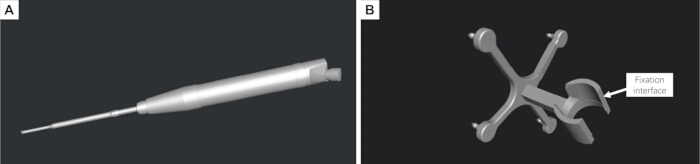
Figure 1: Three-dimensional reconstruction of the surgical instrument and design of the customized instrument-tracking reference frame. (A) Digital three-dimensional (3D) model of the piezoelectric osteotome reconstructed from physical measurements. (B) Customized instrument-tracking reference frame designed to rigidly attach to the surgical instrument and accommodate passive reflective spheres for optical tracking. Please click here to view a larger version of this figure.

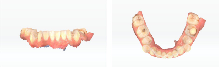
Figure 2: Intraoral scanning of the mandibular dentition. Three-dimensional (3D) intraoral scan of the mandibular dental arch acquired for subsequent registration with the computed tomography (CT)-derived mandibular model and design of the tooth-supported patient-tracking reference frame. Please click here to view a larger version of this figure.

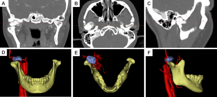
Figure 3: Preoperative computed tomography and three-dimensional reconstruction of the mandibular condylar osteoma. (A–C) Preoperative computed tomography (CT) images in the coronal, axial, and sagittal planes, respectively. (D–F) Corresponding reconstructed three-dimensional (3D) views in the coronal, axial, and sagittal orientations, respectively, showing the spatial relationship between the mandibular condyle, osteoma, and adjacent anatomical structures. Please click here to view a larger version of this figure.

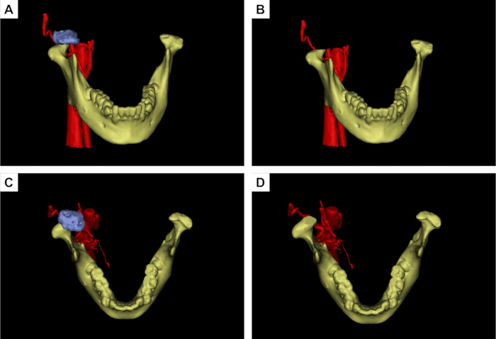
Figure 4: Virtual surgical planning for mandibular condylar osteoma resection. (A,B) Anterior views before and after simulated osteoma resection during virtual surgical planning (VSP). (C,D) Superior views before and after simulated resection. The osteoma is shown in blue, the mandible in yellow, and the adjacent vascular structures in red. The planned osteotomy margin was designed to achieve complete lesion removal while preserving the surrounding normal condylar structures. Please click here to view a larger version of this figure.

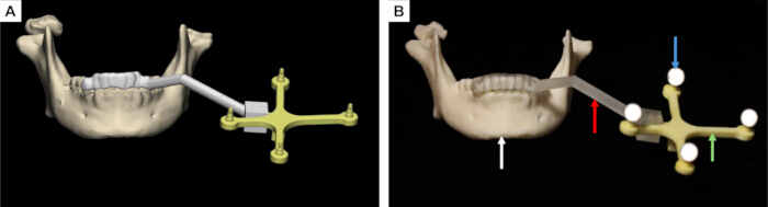
Figure 5: Design and three-dimensional printing of the tooth-supported patient-tracking reference frame. (A) Preoperative virtual design of the customized patient-tracking reference frame. (B) Three-dimensional (3D) printed patient-tracking reference frame. The white arrow indicates the mandibular dentition, the red arrow indicates the supporting arm, the green arrow indicates the reference frame, and the blue arrow indicates the passive reflective spheres used for optical tracking. Please click here to view a larger version of this figure.

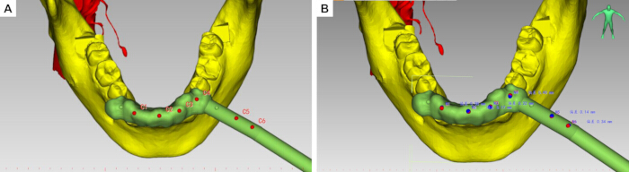
Figure 6: Hemispherical registration depressions and dynamic navigation project configuration. (A,B) Red dots indicate the registration dimples, while blue dots indicate the tool center point (TCP). Please click here to view a larger version of this figure.

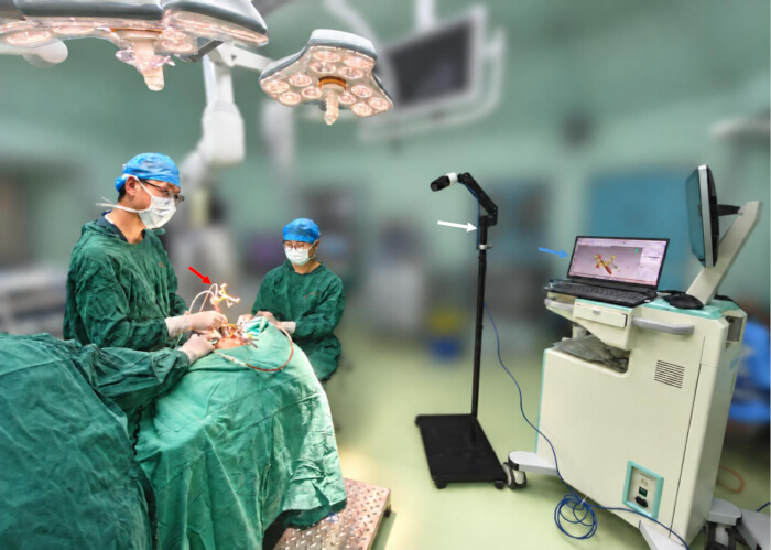
Figure 7: Intraoperative surgical instruments and dynamic navigation setup. The figure shows the main components of the intraoperative dynamic navigation system. The red arrow indicates the piezoelectric osteotome equipped with the customized instrument-tracking reference frame, the white arrow indicates the binocular infrared optical tracking camera, and the blue arrow indicates the computer workstation used for real-time navigation visualization. Please click here to view a larger version of this figure.

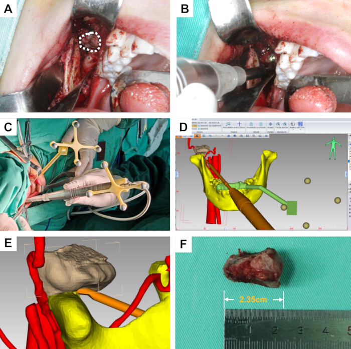
Figure 8: Intraoral condylar osteoma resection under dynamic navigation guidance. (A) Intraoral surgical approach and exposure of the condylar osteoma; the white dashed region indicates the lesion. (B) Osteotomy and tumor resection using the piezoelectric osteotome. (C) Intraoperative spatial arrangement of the patient-tracking reference frame and surgical field. (D) Real-time navigation display showing the position and orientation of the surgical instrument relative to the anatomical structures. (E) Close-up view of real-time instrument localization during navigation-guided osteotomy. (F) Resected osteoma specimen. Please click here to view a larger version of this figure.

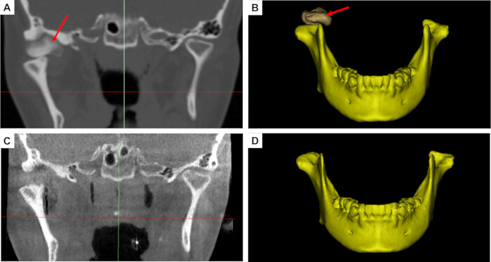
Figure 9: Comparison of preoperative and postoperative computed tomography images and reconstructed three-dimensional models. (A) Preoperative two-dimensional (2D) computed tomography (CT) image showing the condylar osteoma. (B) Preoperative three-dimensional (3D) reconstructed mandibular model. (C) Postoperative 2D CT image obtained after osteoma resection. (D) Postoperative 3D reconstructed mandibular model. The red arrows indicate the location of the osteoma or the corresponding postoperative resection region. Please click here to view a larger version of this figure.

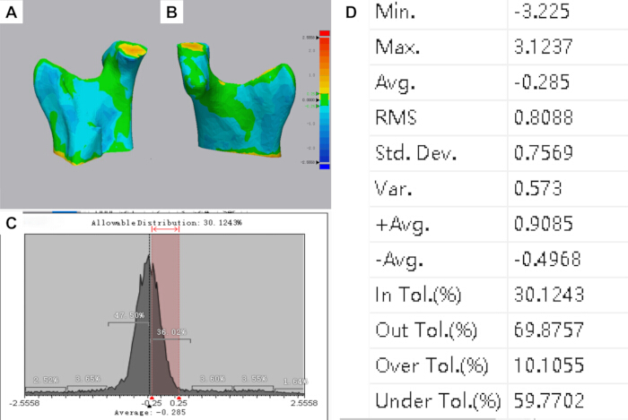
Figure 10: Three-dimensional color-coded surface-deviation analysis between the preoperative virtual surgical plan and postoperative reconstructed model. (A,B) Color-coded surface-deviation maps demonstrating the spatial distribution of discrepancies between the planned and postoperative surfaces. (C) Distribution of surface deviations. The predefined tolerance interval was ±0.25 mm, within which 30.12% of the analyzed surface points were located. (D) Quantitative statistics of the surface-deviation analysis, showing a mean signed deviation of −0.285 mm, standard deviation of 0.757 mm, and root-mean-square deviation of 0.809 mm. Local deviations ranged from −3.225 mm to +3.124 mm. Please click here to view a larger version of this figure.

Discussion

This study presents a novel dynamic surgical navigation protocol with real-time tracking of the operative instrument, successfully applied to transoral resection of mandibular condylar osteomas. This single-case application provides preliminary evidence of the technical feasibility of this approach in the anatomically complex condylar region; however, its clinical effectiveness and generalizability require further evaluation in larger patient cohorts. Condylar osteomas are deeply situated and closely adjacent to critical structures, such as the facial nerve, maxillary artery, articular disc, and periarticular soft tissues of the temporomandibular joint, making conventional surgical exposure and freehand osteotomy exceptionally challenging¹⁰. Surgery in the temporomandibular joint region is conventionally performed through an extraoral preauricular incision; however, the transoral approach has also been reported and, compared with the extraoral approach, may avoid facial nerve injury and facial cutaneous scarring^11,12. Although a transoral approach successfully avoids facial skin scars, it creates a deep, narrow surgical field with restricted direct visualization. Traditional freehand operations make it difficult to determine the precise spatial relationships between the instrument tip, tumor margins, and critical adjacent anatomy. The application of dynamic navigation to transoral condylar osteoma resection successfully addresses these constraints by providing precise spatial guidance for minimally invasive bone removal⁸.

Traditional navigation systems typically rely on handheld positioning pointers for intraoperative registration and localization. Localization is performed solely with the pointer, and no navigational feedback is available during osteotomy using surgical instruments. Such systems only support localization of the initial surgical access, without real-time navigation throughout the osteotomy procedure. Consequently, deviations in the angle and depth relative to the preplanned osteotomy plane may occur, risking injury to adjacent anatomical structures^13,14. To circumvent such discrepancies, current technologies implement real-time navigation via navigation-system-compatible dedicated instruments. This strategy nevertheless introduces a new challenge: specialized instruments have inherent limitations, requiring the preparation of more dedicated instruments for novel surgical scenarios. In contrast, the present method directly integrates the piezoelectric osteotome into the navigation coordinate system, allowing continuous real-time visualization of the working tip and its 3D orientation during osteotomy. Therefore, the principal methodological difference of this approach is not simply the use of dynamic navigation, but the direct navigation of the operative instrument itself to reduce probe-to-instrument transition error.

Tooth-supported or oral appliance-supported reference frames have been previously reported for dynamic navigation in mandibular and dentoalveolar procedures. These approaches provide a noninvasive means of maintaining spatial correspondence between the mandible and the navigation system while avoiding additional skeletal fixation. In the present workflow, the tooth-supported patient-tracking reference frame was incorporated into a navigation protocol specifically developed for transoral condylar osteoma resection and combined with direct real-time tracking of the piezoelectric osteotome.

In executing this protocol, three critical steps directly dictate the final tracking accuracy and surgical safety. First, rigid stabilization of the mandibular patient-tracking reference frame is crucial. Due to mandibular mobility, any structural looseness between the frame and the jaw introduces a coordinate mismatch between preoperative images and the actual anatomy during jaw movement. To mitigate this tracking error, a custom occlusal splint is used to ensure the reference frame moves synchronously with the mandible. For the resin surgical templates used in this workflow, studies have shown that plasma sterilization, povidone-iodine disinfection, and alcohol disinfection have no significant effect on the accuracy of resin surgical templates^15,16. Second, stringent control of spatial registration precision is required. Multi-point sampling and iterative error validation should be performed, particularly near stable and reproducible anatomical landmarks. The subsequent surgical steps must only proceed once the registration error is controlled within the preset threshold. Third, real-time online calibration and trajectory validation of the functional tip are paramount. Because the cutting edge of the piezoelectric osteotome dictates the exact boundaries and depth of the osteotomy, verifying that the on-screen crosshairs match the physical location reduces the risk of injury to deep neurovascular bundles and the joint disc.

Intraoperative troubleshooting mostly centers on managing optical line-of-sight occlusion, which is a common limitation of infrared tracking. In practice, the surgeon's hands, retractors, suction tips, or the handpiece itself can block the optical path between the infrared camera and the markers, causing temporary data loss. To avoid this, proper pre-positioning of the tracking camera is required to ensure continuous coverage. If line-of-sight interruption occurs, the osteotomy must be paused immediately to re-expose the markers and verify frame stability before resuming navigation. Furthermore, instrument calibration errors and reference frame micro-movements are common confounding factors. If an instrument undergoes a tip replacement, mechanical collision, or connector loosening, a prompt recalibration must be executed. Any noticed mismatch between the digital display and physical landmarks, even if minor, warrants an immediate cessation of the procedure and re-verification of the registration accuracy.

Several limitations should be acknowledged. First, this report describes a single representative case; therefore, its clinical feasibility and accuracy findings cannot be generalized. Second, no independent bench- or phantom-based validation of intrinsic system accuracy was performed. Accordingly, the postoperative surface-deviation analysis should not be interpreted as a complete validation of system accuracy. Third, long-term clinical and imaging follow-up remains incomplete because the patient entered orthodontic treatment. Future multicenter studies with larger samples, standardized accuracy endpoints, long-term follow-up, and systematic assessment of the operator learning curve are needed. Therefore, the long-term stability, clear delineation of indications, and postoperative functional recovery associated with this technique require further validation through larger sample sizes and long-term follow-up studies. Future studies should systematically evaluate the operator learning curve for virtual planning, registration, calibration, and hand-eye-screen coordination.

Materials

List of materials used in this article

Name	Company	Catalog Number	Comments
3-0 silk sutures	N/A	N/A	Used for closure of the intraoral surgical incision
3D printer	Suzhou RAYSHAPE Intelligent Technology Co., Ltd.	Edge E2	LCD-based stereolithography three-dimensional printer.(Fabricate the customized patient-tracking reference frame)
3D printer	Suzhou RAYSHAPE Intelligent Technology Co., Ltd.	Edge MAX	LCD-based stereolithography three-dimensional printer.(Fabricate the customized instrument-tracking reference frame)
3-matic	Materialise NV, Technologielaan 15, 3001 Leuven (Heverlee), Belgium.	Research 13.0	Three-dimensional mesh design and editing software
95% industrial grade ethanol	Local chemical supplier, China	N/A	Removal of residual uncured resin
Aoralscan 3i Intraoral 3D Scanner	SHINING 3D Tech Co., Ltd.	Aoralscan 3 CA3-C80046J04	Intraoral three-dimensional scanning device
Cone-beam computed tomography (CBCT) scanner	Quantitative Radiology s.r.1.Verona,Italy	New Tom 3G	Postoperative CT examination
E3D CMF V2.0	Hunan Liuwei Jinghang Digital Technology Co., Ltd., Hunan, China.	version 2.0	Navigation software.
Exocad	SHINING 3D	version 3.3	Dental design software
Geomagic Wrap	3D Systems, Inc.	version 2021	The three-dimensional scanning data processing software
high-precision digital caliper	Local measuring instrument supplier	N/A	Measure the external dimensions of the surgical instrument
methylene blue	N/A	N/A	Used to mark the planned osteotomy and resection boundary
Mimics	Materialise NV, Technologielaan 15, 3001 Leuven (Heverlee), Belgium.	Research 21.0	Three-dimensional reconstruction software
Model resin	Suzhou Laixin 3D Technology Co., Ltd., Suzhou, China.	Model 1 Ivory	Fabricate the customized instrument tracking reference frame
Model resin	Suzhou Laixin 3D Technology Co., Ltd., Suzhou, China.	SG V2	Dental photopolymer model resin (Fabricate the customized patient tracking reference frame)
passive reflective spheres	AIMOOE	Aim Marker-115	Passive reflective spheres
Piezoelectric Bone Surgery System	SMTP Technology Co., Ltd., China	XD880A	Used for intraoral resection of the condylar osteoma
Piezoelectric osteotome tip	SMTP Technology Co., Ltd., China	FDF02806510C	Used for osteotomy and resection of the condylar osteoma
Polaris Lyra	NDI	N/A	6-degree-of-freedom optical navigation tracker
povidone-iodine solution	N/A	N/A	Used for preoperative disinfection of the surgical field
Proplan CMF	Materialise NV, Technologielaan 15, 3001 Leuven (Heverlee), Belgium.	version 3.0	Image processing and surgical planning software
rubber drain strip	N/A	N/A	Used for postoperative wound drainage
ShapeCure+	RAYSHAPE	N/A	Post-curing chamber for ultraviolet light curing
ShapePanel	RAYSHAPE	N/A	Dental 3D printing preprocessing slicing software
silicone mouth gag	N/A	N/A	Used to maintain mouth opening and improve intraoral surgical exposure
SolidWorks 2025	Dassault Systèmes	version 2025	Three-dimensional modeling software
Spiral computed tomography (CT) scanner	Toshiba Medical Systems Corporation, Otawara, Japan	Aquilion CXL 64-row 128-slice	Preoperative CT evaluation
tool characterization software	NDI	Cygna-6D	Tool characterization software

References

- Valente L, Tieghi R, Mandrioli S, Galiè M. Mandibular condyle osteoma. Ann Maxillofac Surg. 2019;9(2):434-438.
- De Souza NT, et al. An unusual osteoma in the mandibular condyle and the successful replacement of the temporomandibular joint with a custom-made prosthesis: A case report. BMC Res Notes. 2017;10(1):727.
- Nilesh K, Vande A, Reddy S. Central compact osteoma of mandibular condyle. BMJ Case Rep. 2020;13(2):e233082.
- Bi R, et al. Expert consensus on treatment of condylar hyperplasia and secondary dento-maxillofacial deformities. Int J Oral Sci. 2026;18(1):45.
- Nam H, Ko DE, Shin KS. A multidisciplinary approach to treatment for osteochondroma of the mandibular condyle and oral rehabilitation: A case report. Medicine (Baltimore). 2025;104(37):e44359.
- Marliere DA, et al. Accuracy between virtual surgical planning and actual outcomes in orthognathic surgery by iterative closest point algorithm and color maps: A retrospective cohort study. Med Oral Patol Oral Cir Bucal. 2019;24(2):e243-e253.
- Wang F, Cai X, Sun W, Chen C, Meng L. Application of dynamic navigation technology in oral and maxillofacial surgery. Clin Oral Investig. 2024;29(1):13.
- Demian N, Pearl C, Woernley TC 3rd, Wilson J, Seaman J. Surgical navigation for oral and maxillofacial surgery. Oral Maxillofac Surg Clin North Am. 2019;31(4):531-538.
- Cassoni A, et al. Three-dimensional comparison of the maxillary surfaces through ICP-type algorithm: Accuracy evaluation of CAD/CAM technologies in orthognathic surgery. Int J Environ Res Public Health. 2022;19(18):11834.
- Chen S, et al. Lateral molar approach-driven transoral endoscopic procedure for benign infratemporal fossa tumor resection. J Vis Exp. 2025;222:e68672.
- Hernández-Alfaro F, Méndez-Manjón I, Valls-Ontañón A, Guijarro-Martínez R. Minimally invasive intraoral condylectomy: Proof of concept report. Int J Oral Maxillofac Surg. 2016;45(9):1108-1114.
- Deng M, Long X, Cheng AHA, Cheng Y, Cai H. Modified trans-oral approach for mandibular condylectomy. Int J Oral Maxillofac Surg. 2009;38(4):374-377.
- He Y, Huang T, Zhang Y, An J, He L. Application of a computer-assisted surgical navigation system in temporomandibular joint ankylosis surgery: A retrospective study. Int J Oral Maxillofac Surg. 2017;46(2):189-197.
- Wu J, et al. Patient-specific dynamic reference frame for navigation-assisted surgery in mandible: A novel noninvasive technical method. Front Bioeng Biotechnol. 2025;13:1577321.
- Di Spirito F, et al. Dynamic computer-aided navigation system in dentoalveolar surgery and maxillary bone augmentation in a dental setting: A systematic review. Healthcare (Basel). 2025;13(14):1730.
- Lan D, Zhou Z, Yang Y, Xu Z, Man Y. Influence of material, sterilization, and disinfection on the accuracy of three-dimensional printed surgical templates: An in vitro study. Clin Oral Implants Res. 2024;36(2):191-201.