本文介绍了可调控的三维共缠结肌动蛋白丝与微管复合网络的构建与表征方法。该复合材料在肌球蛋白II和驱动蛋白马达的驱动下发生主动重构和弹道运动,并可通过调节肌动蛋白、微管、马达蛋白和被动交联分子的相对浓度进行调控。
本文内容
勘误通知
Important: There has been an erratum issued for this article. View Erratum Notice
摘要
摘要
由相互作用的半柔性肌动蛋白丝和刚性微管网络组成的复合细胞骨架,利用如肌球蛋白II和驱动蛋白等马达蛋白来重构结构并产生作用力,从而驱动细胞迁移、胞质分裂、黏附以及机械感知等关键过程。尽管肌动蛋白与微管之间的相互作用对细胞骨架的多功能性和适应性至关重要,但目前对其与肌球蛋白和驱动蛋白活性之间协同作用的理解仍处于初步阶段。本文介绍了如何构建可调控的三维复合网络,其中肌动蛋白丝与微管共缠结,并在肌球蛋白II和驱动蛋白马达的作用下发生主动重构和弹道式运动,且可通过调节肌动蛋白、微管、马达蛋白和被动交联分子的相对浓度进行调控。文中还详细描述了对微管和肌动蛋白丝进行荧光标记的实验方案,以通过多光谱共聚焦成像最有效地观察复合结构的重构过程与运动行为。最后,展示了可用于定量表征非平衡态结构、动力学及力学特性的数据分析方法的结果。重建并研究这一可调的仿生平台,为理解马达蛋白活性、复合力学性能与丝状结构动力学的耦合如何导致从有丝分裂、细胞极化到机械感知等多种细胞过程提供了重要见解。
引言
细胞骨架是由相互作用的生物大分子组成的动态复合网络,为细胞提供结构和力学支持。相关的分子马达和结合蛋白可重构并调节细胞骨架,使细胞能够生长、改变形状、硬化、移动甚至自我修复,从而实现从迁移、分裂到机械感知等多种细胞过程1,2。除了在细胞生物物理学中的重要意义外,细胞骨架也是活性物质的典型范例,其在材料科学中的潜在应用广泛,涵盖伤口愈合、药物递送、过滤技术以及软体机器人等领域1,3,4,5,6,7,8,9。
赋予细胞骨架独特结构和力学多样性以及多功能性的两个关键特征是:1)其复合性质,包含多种相互作用的蛋白质纤维,如半柔性肌动蛋白纤维和刚性微管,以及与之相关的结合蛋白和交联蛋白3,5,10;以及其持续重构、移动、粗化和做功的能力 通过 耗能马达蛋白(如肌球蛋白和驱动蛋白)对丝状蛋白进行推拉作用1,7,11,12,13尽管这种精妙的复杂性使细胞骨架能够介导细胞运动、胞质分裂和伤口愈合等多样化的过程3,6,7,11,这会妨碍研究人员重现该特征的能力 体内 重建细胞骨架的特征 体外 系统。
当前前沿的重建研究主要集中在由缠结和交联的肌动蛋白丝与微管组成的复合物上3,10,14,15,16,17,产生作用力的肌动蛋白-肌球蛋白网络2,8,18,19,20,21以及由驱动蛋白-微管相互作用驱动的活性向列相22,23,24,25,26稳态肌动蛋白-微管复合物已被证明具有涌现的力学特性15,16,27,与单组分系统相比,具有增强的丝状物移动性和更高的刚度27. 关于研究 体外 肌动球蛋白系统已报道了多种结构和动态特性,这些特性依赖于肌动蛋白、肌球蛋白和交联蛋白的浓度28,29,30,31例如,在充分交联的情况下,肌动球蛋白网络会发生大尺度的收缩和粗化2,28,30,32,33,34,35,36而无交联剂时,网络会表现出快速的失稳流动和破裂19,29. 已有报道指出,利用驱动蛋白马达簇交联并牵拉微管束的重建微管基活性向列相系统可表现出持久的湍流流动、延伸、屈曲、断裂与自愈合现象12,22,23,24,25,37,38,39,40,41,42,43,44,45,46,47.
最近的研究表明,由肌球蛋白II小丝驱动的肌动蛋白-微管复合物相比无交联剂的肌动蛋白-肌球蛋白网络所表现出的无序流动和网络破裂,能够实现更有序的收缩和更高的网络完整性17,26,48。此外,当肌动蛋白和微管以相近浓度存在时,复合物的力学稳定性与力生成能力达到最佳。在此配比范围内的关键涌现特性包括增强的机械强度26、肌动蛋白与微管的协调运动26、持续稳定的收缩以及介观尺度的结构重组17。
本文描述了构建和调控微管与肌动蛋白丝共缠结且交联的复合物的实验方案,这些复合物分别由作用于肌动蛋白丝的肌球蛋白II小丝和作用于微管的驱动蛋白簇驱动,使其处于非平衡状态(图1)。通过调节纤维、马达蛋白和交联分子的相对浓度,可调控此类复合物的动力学行为、结构特征和力学性能,从而呈现出丰富的相态行为,包括对流和湍流流动、各向同性收缩、加速、减速、相分离、刚度增强、松弛以及破裂。本研究的重点在于制备并调控这类活性细胞骨架复合物。然而,为了帮助研究人员对标定和表征所描述的活性复合物,本文还详细介绍了利用多光谱共聚焦显微镜进行有效成像的方法。最后,展示了可用于测量复合物动力学、结构和力学特性的关键计算分析方法的结果。鼓励研究人员采用这些方法——包括差分动力学显微术(DDM)、空间图像自相关分析(SIA)和粒子图像测速技术(PIV)——因为这些方法已针对复合物复杂的动力学行为和结构多样性进行了优化17,26,49。
以下步骤重点介绍复合材料的制备及其利用共聚焦显微镜进行成像。有关采集后数据分析和光镊测量的实验方案可参见先前的研究工作。 17,26,48,50, 应要求提供。所有材料均列于随附的材料表中。
方案
1. 准备硅烷化盖玻片和显微镜载玻片,以防止蛋白质吸附到样品池表面
注意:此过程需要2天。硅烷化载玻片可提前最多1个月制备,以备后续使用。
- 将1号盖玻片(24 mm × 24 mm)和载玻片(1英寸 × 3英寸)放入可适配等离子清洗仪的专用支架中,将支架放入等离子清洗仪中运行20分钟。
- 将盖玻片和载玻片转移至仅用于硅烷处理的专用支架中,并将支架放入玻璃容器内,按以下步骤清洗玻片:
- 将盖玻片和载玻片浸入100%丙酮中1小时,随后浸入100%乙醇中10分钟。
- 将盖玻片和载玻片浸入去离子水(DI)中5分钟,重复清洗步骤共三次。
- 将盖玻片和载玻片浸入新配制的0.1 M KOH溶液中15分钟,再浸入新鲜去离子水中5分钟,重复此步骤共三次。
- 将盖玻片和载玻片在空气中干燥10分钟,随后对已清洗的盖玻片和载玻片进行硅烷处理,以形成疏水表面,具体步骤如下:
注意:以下步骤需在通风橱中完成。- 将 干燥的盖玻片和载玻片浸入2%硅烷(溶于甲苯)中5分钟。使用漏斗将硅烷溶液倒回指定瓶中,可重复使用最多五次。
- 将盖玻片和载玻片浸入100%乙醇中5分钟,随后更换为新鲜乙醇,再次浸入5分钟。
- 将盖玻片和载玻片浸入新鲜去离子水中5分钟,重复乙醇和去离子水洗涤步骤共三次,每次均使用新鲜乙醇和去离子水。最后将盖玻片和载玻片在空气中干燥10分钟。
2. 制备由肌球蛋白迷你丝驱动的活性肌动蛋白-微管复合物
- 去除无活性的肌球蛋白 通过 肌动蛋白丝结合及拉下实验 通过 超速离心,具体步骤如下。
- 将肌动蛋白聚合为纤维。使用精密微量移液器和无菌吸头,在微量离心管中加入: 1.87 µL 去离子水 1.3 µL 10倍G缓冲液 1.3 µL 10倍F缓冲液 1.63 µL 4 M KCl 溶液 4.53 µL 的肌动蛋白(47.6 µM),以及 1.08 µL 的 100 µM phalloidin
注意:为了确保充分聚合,肌动蛋白浓度及肌动蛋白与鬼笔环肽的摩尔比应 18.4 µM 分别为2:1。 - 轻轻吹打溶液以混匀,然后在避光条件下冰浴放置 ≥1 h。将超速离心机预冷至 4 °C. 从 -80 °C 取出肌球蛋白等分试样80 °C 置于冰上。
注意:在肌动蛋白聚合的同时,执行步骤 2.2。 - 在肌动蛋白聚合 ≥1 h 后,加入 1.3 µL 10 mM ATP 2 µL 的 19 µM 肌球蛋白与聚合的肌动蛋白结合。
注意:肌动蛋白与肌球蛋白的摩尔比应为 >5,以确保充分去除无活性的肌球蛋白马达(即失活的头部)。 - 轻轻吹打溶液以混匀,转移至超速离心管中。
离心 4 °C 和 121,968 x g 30分钟
- 将肌动蛋白聚合为纤维。使用精密微量移液器和无菌吸头,在微量离心管中加入: 1.87 µL 去离子水 1.3 µL 10倍G缓冲液 1.3 µL 10倍F缓冲液 1.63 µL 4 M KCl 溶液 4.53 µL 的肌动蛋白(47.6 µM),以及 1.08 µL 的 100 µM phalloidin
- 按如下所述制备肌动蛋白丝与微管的共缠结复合网络。
注意:在肌球蛋白沉降实验(步骤 2.1.4)开始前 30 分钟进行。- 将加热块设定至 37 °C使用精密移液器和无菌吸头,将以下成分加入微量离心管中: 13.9 µL PEM的 3 µL 含 1% Tween20, 1.55 µL 的 47.6 µM 肌动蛋白, 0.36 µL 的 34.8 µM R-肌动蛋白, 0.3 µL 250 mM ATP 0.87 µL 的 100 µM 鬼笔环肽, 1.91 µL 5-488-微管蛋白 0.3 µL 100 mM GTP 0.75 µL 的 200 µM 紫杉醇,加至总体积 23 µL.
注意:所列出的肌动蛋白和微管蛋白浓度是针对复合物的 2.9 µM 肌动蛋白和 2.9 µM 微管蛋白。总蛋白浓度为 c = cA + cT = 5.8 μM 以及摩尔肌动蛋白分数为 cA/(cA + cT) = ΦA = 0.5。请参见步骤 2.5 以调整这些数值。 - 轻轻吹打溶液以混匀,并置于 37 °C 避光条件下,37℃金属浴中孵育1小时。
- 将加热块设定至 37 °C使用精密移液器和无菌吸头,将以下成分加入微量离心管中: 13.9 µL PEM的 3 µL 含 1% Tween20, 1.55 µL 的 47.6 µM 肌动蛋白, 0.36 µL 的 34.8 µM R-肌动蛋白, 0.3 µL 250 mM ATP 0.87 µL 的 100 µM 鬼笔环肽, 1.91 µL 5-488-微管蛋白 0.3 µL 100 mM GTP 0.75 µL 的 200 µM 紫杉醇,加至总体积 23 µL.
- 按照以下说明准备共聚焦成像实验所需的样品腔室。
注意:在等待期间完成步骤 2.1.4 和 2.2.2。- 将两张硅烷化载玻片并排置于关闭的加热板上,在载玻片上相距约3 mm处横向放置两条热塑性封片膜,再将两张硅烷化盖玻片覆盖于热塑性封片膜上,形成样品腔室。
- 将热板调至低温档,加热至盖玻片通过熔化的热塑性封片膜牢固粘附于载玻片上(约1–2分钟)。均匀施压以确保粘合效果,同时保持约100 µm 两个表面之间的间距。
- 移除腔室并关闭加热板。用(+)和(-)标记腔室。(+)腔室用于活性样品(含肌球蛋白),(-)腔室用于对照(无肌球蛋白)。确保每个腔室可容纳 ≤10 µL 液体。
- 按照下述方法制备待成像样品。
注意:在完成步骤 2.1 和 2.2 后,必须立即执行此步骤。- 小心地从超速离心机(步骤 2.1.4)中取出肌球蛋白-肌动蛋白样品,并立即用移液器吸取上层 7.5 µL 上清液转移至新的微量离心管中。
- 从热块中取出肌动蛋白-微管样品,并轻轻混匀 1.5 µL 10× D-葡萄糖, 1.5 µL 10x GOC 的 1.5 µL 1 mM 比比斯坦溶液分成两份 13.7 µL 分装并标记为 (+) 和 (-)。
- 混合 1.28 µL 将步骤 2.4.1 中的上清液加入 (+) 分装管中。混合 1.28 µL 将DI加入至(-)等分试样中。缓慢将每种溶液流入相应的腔室(步骤2.3) 通过 毛细作用。注意避免将气泡引入通道中。
- 用快干环氧树脂或紫外胶密封每个通道的两个开口端。在将样品置于显微镜前,确保胶水完全干燥。按照步骤3所述立即进行成像。
注意:UV 胶具有优势 因为它在紫外光照射下几乎瞬间固化。然而,由于blebbistatin对紫外线敏感,必须仅使用小型紫外光笔对胶水局部照射(在样品腔边缘处),以避免使blebbistatin失活。
- 可选:调整蛋白质浓度以调控复合物的动力学特性和结构。
注意:如果需要,可对上述步骤进行如下调整,以改变肌动蛋白、微管和肌球蛋白的浓度。- 除步骤 2.2.1 和 2.4.3 中所述修改外,其余步骤均按照上述描述进行。
- 通过改变肌动蛋白和微管的浓度,从而进行调节 c 和 ΦA,可根据需要增加或减少步骤 2.2.1 中所用的肌动蛋白、R-actin 和 5-488-tubulin 的体积26. 在改变肌动蛋白浓度时,应按比例调整R-actin和鬼笔环肽的摩尔浓度,以保持与肌动蛋白的摩尔比不变。同时调整PEM的体积,使混合物的最终体积保持不变 23 µL所有其他组分的体积和浓度保持不变。
- 通过调整第 2.4.3 步中加入 (+) 分样中的肌球蛋白体积,以调节肌球蛋白浓度。相应调整加入 (-) 分样中的去离子水体积。调整第 2.2.1 步中的 PEM 体积,以补偿肌球蛋白 (+) 和去离子水 (-) 体积的增减,确保每个样品 ((+) 和 (-)) 的最终体积为 14.98 μL.
3. 使用共聚焦显微镜对活性复合材料进行成像与表征
- 为观察步骤2中制备的肌动球蛋白-微管复合物,使用配备60倍、1.4数值孔径(NA)油浸物镜的激光扫描共聚焦显微镜(LSCM)或类似显微镜。为在不同荧光通道中同时观察肌动蛋白纤维和微管,分别采用561 nm激光配合565/591 nm激发/发射滤光片,以及488 nm激光配合488/525 nm激发/发射滤光片。
- 将样品室置于显微镜上,使控制通道正对物镜下方。确保物镜与盖玻片之间有油相界面。
- 使用载物台控制装置将对照复合样品调至清晰对焦,然后找到样品室的上下两个表面。将 z 轴位置移至样品室中心。检查是否存在清晰的丝状网络结构,如图所示。 图2.
- 在观察对照室的同时,调节各激光器的强度,以便同时观察肌动蛋白丝和微管。应保持尽可能低的激光强度,以防止光漂白(在肌动蛋白通道中更为明显)和串色(通常从微管通道渗入肌动蛋白通道)。
- 为表征非活性对照样本,采集三段256 × 256像素的方形像素时间序列(视频),213 µm x 213 µm) 以2.65帧/秒的速度采集图像,总帧数不少于1000帧。每个时间序列在样品腔的不同区域采集,区域之间间隔不少于≥500 µm确保可检测到的运动最小,且无流动或结构重组。
- 关闭488 nm激光器,使用载物台控制装置移动至(+)室。
- 使用 568 nm 激光,在 (+) 通道中观察微管,以确保网络结构正常形成(图2)并确定样品室的轴向中心(该位置可能与对照室的中心 z 位置不同)。
- 打开488 nm激光器,并对上述步骤3.5进行修改后重复操作。采集时间序列最长至45分钟,在样品移出视野、发生破裂或发生光漂白时停止采集。记录5–10个时间序列,并记录每个时间序列相对于第一个时间序列开始时刻的时间。
- 使用 DDM、SIA 和 PIV 分析数据,具体方法如所述 图3, 图4, 图5,以及先前17,48,50,51.
注意:488 nm 激光通过解除对肌球蛋白ATP酶活性的抑制(即失活blebbistatin)实现局部激活,因此仅应在实验开始时开启 数据采集时,将 t = 0 设为时间序列的起始点。这些采集参数已针对差分动态显微镜(DDM)分析进行了优化,方法与先前研究一致。26.
4. 由驱动蛋白马达驱动的活性肌动蛋白-微管复合物的制备
注意:以下步骤将创建由驱动蛋白马达或驱动蛋白与肌球蛋白50共同驱动而偏离平衡态的肌动蛋白-微管复合物。
- 按照下述方法准备驱动蛋白和肌球蛋白马达。
- 若需加入肌球蛋白,请执行步骤 2.1。
- 为形成可结合并施加作用力于微管对之间的驱动蛋白马达簇,使用微量移液器和无菌移液器吸头,向一个无菌的1.5 mL微量离心管中加入以下成分:1.16 µL PEM 2.74 µL 8.87 µM 驱动蛋白二聚体, 7.29 µL 83.3 µM NeutrAvidin 0.81 µL 2 mM DTT。用移液器轻轻吹打混匀,避光孵育(使用黑色微量离心管或用锡箔纸包裹)30分钟,于 4 °C.
注意:驱动蛋白二聚体与 NA 的摩尔比为 1:25。
- 按照步骤2.3准备样品腔室,制备三个腔室而非两个。在驱动蛋白孵育(步骤4.1.2)和肌球蛋白超速离心(步骤4.1.1)期间执行此步骤。
- 制备肌动蛋白纤维与微管的共缠结复合网络。
- 将加热块设定为 37 °C使用微量移液器和无菌吸头,将以下成分加入一支无菌的1.5 mL微量离心管中: 3.21 µL PEM, 4.5 µL 1% Tween20 2.18 µL 的 47.6 µM 肌动蛋白, 3.46 µL 5-R-微管蛋白,4.5 µL 100 mM ATP 4.5 µL 10 mM GTP 1.13 µL 的 200 µM 紫杉醇,以及 1.57 µL 的 20 µM 488-鬼笔环肽。确保总体积为 25 µL.
- 轻轻吹打溶液以混匀,并置于 37 °C 避光条件下在加热块中孵育1小时。将离心管从加热块中取出,使用微量移液器轻轻混匀 0.84 µL 100分之 μM 鬼笔环肽。室温避光孵育5-10分钟。
注意:在此步骤中加入鬼笔环肽,而非步骤 4.3.1,可改善肌动蛋白丝的荧光标记效果,因为 488-鬼笔环肽无需与未标记的鬼笔环肽竞争肌动蛋白结合位点。
- 为共聚焦成像制备活性复合材料。
- 添加 1.13 µL 的 200 μM blebbistatin, 1.35 µL 10倍浓度的Glu,以及 1.35 µL 将10倍浓度的GOC溶液加入步骤4.3.2所得溶液中,轻轻吹打混匀。将溶液均分为三份 10 µL 分装并标记为 (K)、(K+M) 和 (-)。
- 混合 2.54 µL 将步骤 2.1.4 中的肌球蛋白加入 (K+M) 等分试样中。混匀 2.54 µL 将 PEM 分装至 (K) 和 (-) 管中。
- 使用微量移液器和无菌吸头添加 2.5 µL 将4.1.2步骤中的驱动蛋白聚集体分别加入到(K)和(K+M)分装液中。用移液器上下吹打混匀。充分混匀 2.5 µL 使用相同技术将 PEM 转换至 (-)。
注意:所列出的肌动蛋白和微管蛋白浓度适用于复合物 2.32 µM 肌动蛋白和 3.48 µM 微管蛋白。总蛋白浓度为 c = cA + cT = 5.8 μM 以及摩尔肌动蛋白分数为 cA/(cA + cT) = ΦA = 0.4。驱动蛋白和肌球蛋白的浓度为 0.35 µM 和 0.47 µM,分别参见步骤 2.5 中关于调整 c 的通用指南A,cT,c,和 ΦA. - 使用微量移液器,将每种溶液缓慢注入已制备的样品室(步骤 4.2)对应的通道中 通过 毛细作用。缓慢而轻柔地向下按压移液管,以避免将气泡引入通道中。
- 用快干环氧树脂或紫外固化胶密封每个通道的两个开口端。在将样品置于显微镜前,确保胶体完全干燥。
注意:此步骤需快速完成,以尽量减少驱动蛋白在未受监测情况下发挥作用的时间。因此,建议使用1分钟内固化的环氧树脂(而非5或10分钟固化的类型)。在此方面,紫外光固化胶具有优势,因其在紫外光照射下可几乎瞬间固化。
- 在完成第3步后立即制备用于成像的样品,但需进行以下重要修改。由于驱动蛋白(kinesin)不受光激活控制,其在第4.4.3步之后即立即开始发挥作用,因此将此时刻标记为 t = 0。为了尽可能接近初始非活性状态(t = 0)对复合物进行成像,应首先对(K)和(K+M)通道进行成像,并记录从第4.4.3步到数据采集开始(第3.8步)之间经过的时间。实际操作中,该时间间隔约为5 min。
5. 将被动交联剂掺入活性复合材料
注意:这些步骤描述了如何使用生物素标记的肌动蛋白和微管蛋白亚基以及中性亲和素(NA)在步骤4所述的活性复合物中被动交联肌动蛋白与肌动蛋白(A-A)或微管与微管(M-M)。
- 制备含有生物素化蛋白(生物素-肌动蛋白或生物素-微管蛋白)、NA 和生物素的 A-A 或 M-M 交联剂复合物,其比例为 2:2:1(生物素-肌动蛋白/微管蛋白 : 生物素 : NA)。此步骤应在第 4 步之前开始。
- 对于 A-A 交联剂,使用微量移液器和无菌移液吸头,向微量离心管中加入 2 µL 的 11.6 µM 生物素-肌动蛋白、1.39 µL 的 8.33 µM NA、2.27 µL 的 1.02 µM 生物素,以及 4.34 µL 的 PEM。通过上下吹打轻轻混匀。
- 对于 M-M 交联剂,使用微量移液器和无菌移液吸头,向微量离心管中加入 1.86 µL 的 4.55 µM 生物素-微管蛋白、1.11 µL 的 8.33 µM NA、1.82 µL 的 1.02 µM 生物素,以及 5.21 µL 的 PEM。通过上下吹打轻轻混匀。
- 用热塑性密封膜包裹第 5.1.1 和/或 5.1.2 步骤中的离心管,形成防水密封。将管子放入浮力浮板中,并置于设定为 4 °C 的温控超声水浴中。
- 在 4 °C 下超声处理 90 分钟。实际操作中,最好将超声仪置于冷室中,并在超声水浴中加入冰袋以维持低温。
- 为将交联剂复合物掺入成像样品,请遵循第 4.3 步,并根据以下说明修改第 4.3.1 步,分别用于 A-A 交联(第 5.2.1 步)或 M-M 交联(第 5.2.2 步)。
- 对于 A-A 交联,在微量离心管中混合以下组分:1.94 µL PEM、4.50 µL 1% Tween20、2.18 µL 47.6 µM 肌动蛋白、3.46 µL 45.5 µM 5-R-微管蛋白、1.13 µL A-A 交联剂(第 5.1.1 步)、4.50 µL 100 mM ATP、4.50 µL 10 mM GTP、1.13 µL 200 µM 紫杉醇,以及 1.57 µL 20 µM 488-鬼笔环肽。确保总体积为 25 µL。
- 对于 M-M 交联,在微量离心管中混合以下组分:1.97 µL PEM、4.50 µL 1% Tween20、2.18 µL 47.6 µM 肌动蛋白、3.76 µL 45.5 µM 5-R-微管蛋白、1.13 µL 经 1:4 稀释的 M-M 交联剂(第 5.1.2 步)、4.50 µL 100 mM ATP、4.50 µL 10 mM GTP、1.13 µL 200 µM 紫杉醇,以及 1.57 µL 20 µM 488-鬼笔环肽。确保总体积为 25 µL。
- 按照第 4.3.2–4.5 步操作,使用特定浓度,使交联剂与肌动蛋白的摩尔比为 RA = 0.02,交联剂与微管蛋白的摩尔比为 RT = 0.005。这些 RA 和 RT 值可使交联剂在肌动蛋白丝和微管上的间距相近(dA
 60 nm 和 dMT 67 nm),估算公式为 dA = I单体/2RA,其中 I单体 为肌动蛋白单体的长度;dMT = I环/26RT,其中 I环 为由 13 个微管蛋白组成的环的长度15,17。
结果
为确定活性复合材料制备是否成功(图1),为了表征其动态行为和结构,需使用至少具备两个荧光通道的激光扫描荧光显微镜,同时观察微丝和微管图2 和 图6)。复合物中的所有肌动蛋白丝和微管均为稀疏标记,而非像通常做法那样掺入示踪亮丝 体外 研究。该方法可确保所测得的动力学和结构特征反映的是复合物本身,而非在不同于复合物形成的条件下生成的示踪剂。因此,通常无法分辨单个的肌动蛋白丝和微管,图像所呈现的主要是介观尺度的网络结构图2 和 图6).
该标记方法已针对空间图像自相关(SIA)和差分动态显微镜(DDM)分析进行了优化,可用于研究倒易傅里叶空间中的动力学与结构(图4、图5 和 图8)52,53,54,55。粒子图像测速(PIV)也可用于描绘和表征动力学过程与流场(图3 和 图7),但为消除密集、低信噪比图像中噪声引起的错误矢量,PIV需要像素合并(空间分辨率较低)以及更大的时间滞后增量(时间分辨率较低),其空间和时间分辨率均低于SIA和DDM。尽管如此,PIV仍推荐用于流场的定性分析以及对DDM结果的验证(图4 和 图8)26,50。
本文提供了利用这些分析方法(即 DDM、SIA、PIV)对所描述网络进行样品表征的示例,以帮助研究人员采用类似分析手段对其样品进行基准测试与特征分析。然而,这些技术的详细描述不在本研究的范围之内。有关在这些及其他类似系统上实施 DDM 的详细说明,包括用户友好的 Python 代码,请参阅先前的研究工作17,26,49,50 及其中引用的参考文献。关于如何在本文所述系统上执行 SIA 和 PIV 的具体细节,读者可参考先前的研究工作17,50。
应进行以下所述的多个对照实验,以确保复合物按预期发挥作用。不含肌球蛋白或驱动蛋白的复合物应基本保持静止,仅表现出微小的热波动或漂移。肌动蛋白纤维与微管应呈现共缠绕且均匀分布的状态,在约 200 µm × 200 µm 的视野范围内,肌动蛋白和微管应极少出现成束、聚集或相分离现象(图 2,最左侧)17。对于含有肌球蛋白但未暴露于 488 nm 光(以去除非肌球蛋白抑制剂blebbistatin的抑制作用)的复合物,也应观察到类似结果。
加入肌球蛋白并暴露于488 nm光照后,复合材料发生收缩,该收缩在很大程度上是各向同性的,且肌动蛋白与微管蛋白的表现相似,这一点可通过肌球蛋白活性前后显微镜图像(图2)以及活性过程中不同时刻对应的PIV流场图(图3)观察到。为确定运动模式属于弹道式、扩散式、亚扩散式等类型,需评估由DDM方法获得的特征去相关时间 τ(q)随波矢量(即倒易空间)的变化关系。具体方法详见先前文献17,26,49。图4还展示了如何利用DDM对这些复合材料进行表征。幂律关系τ(q)~1/vqβ中,当 β = 1时,表明运动为弹道式,速度为v。 作为参考, β = 2对应扩散动力学,其中v为扩散系数。所有活性复合材料均表现出弹道式标度行为(图4A),其运动速度可通过肌动蛋白和肌球蛋白的浓度进行调控(图4B),并在活性过程中随时间变化,表现为加速或减速(图4C,D)。
网络重构与聚类,在 图2 肌动蛋白和肌球蛋白浓度越高,这一现象越明显, 可使用SIA进行表征,如图所示 图5,此前已有描述17,48,50简而言之,相关长度 ξ,即图像中特征尺寸的表征量,可通过拟合每个空间强度自相关曲线来确定 g(r) 距离的指数函数 r 像素之间。较大的 g(r)峰在更长距离上持续存在,表明存在较大的结构特征(即单根纤维的束状结构或簇状聚集)。如图所示 图5,对于较高的肌动蛋白组分和肌球蛋白浓度,显著的结构重组和聚集反映在增加中 ξ 随着时间的推移。
活性复合材料的黏弹性特性及其非线性力学响应也可通过光镊微流变学(OTM)进行测量。然而,这些实验的方案及代表性结果不在本研究的讨论范围内。感兴趣的读者可参考先前的研究工作48,56,其中详细描述了如何开展OTM测量以及预期的结果。
利用上述相同的实验与分析工具程序,下文将描述当驱动蛋白马达和生物素化核酸交联剂被引入复合物时,其动力学和结构发生的变化(图6、图7 和 图8)。图6 展示了仅由驱动蛋白(K)驱动或由驱动蛋白与肌球蛋白共同驱动(K+M)的复合物的代表性共聚焦图像,其中包含或不包含对肌动蛋白丝或微管的被动交联(XL)。
将驱动蛋白引入复合物后,最初产生的动态行为和重构过程与肌球蛋白驱动的复合物相似,如图7(第一类)上排所示。然而,其动态通常会转变为大规模的各向异性流动(图7 中排,第二类)、加速与减速现象(图7 下排,第三类)。这些特征在5–30分钟后会伴随介观尺度的簇集与聚集行为(图6 和 图8B)。由PIV生成的流场图和时间彩色图(图7)展示了各向同性重构(第一类,上图面板)、定向流动(第二类,中图面板)以及双向加速(第三类,下图面板)的示例。
不同活动时间点下肌动蛋白和微管的运动速度测定 通过 拟合到 τ(q)曲线,显示先加速后减速的过程(图8),这取决于 交联。如图中所示 图8,当两种运动蛋白均被引入时,其动力学实际上比仅含驱动蛋白的复合物更慢,并且介观尺度流动的起始存在延迟。在整个活性持续期间,肌球蛋白还促进了肌动蛋白与微管网络更均匀的相互渗透,以及更少的聚集和重构现象。这些效应可在以下图像中观察到 图6 并通过计算随时间变化的相关长度进行量化 通过 SIA在肌球蛋白存在时通常较小图8B).
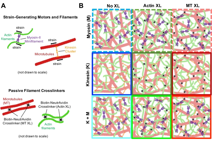
图 1.具有多种力生成马达和被动交联剂的活性肌动蛋白-微管复合物的设计与表征。 (A) 肌动蛋白单体和微管蛋白二聚体在摩尔浓度 cA 和 cT 分别为 0.73–11.6 μM、肌动蛋白摩尔分数 ΦA = cA / (cA + cT) = 0、0.25、0.5、0.75 和 1 的条件下共聚合,形成肌动蛋白丝(绿色)和微管(红色)的共缠结网络。通过使用 NA 实现被动交联,以连接生物素化的肌动蛋白丝(Actin XL)或微管(MT XL),其交联剂与蛋白的摩尔比分别为 RA = 0.01–0.08 和 RMT = 0.001–0.01(分别对应肌动蛋白和微管)。肌球蛋白-II 小丝(紫色)和驱动蛋白簇(橙色)的浓度分别为 cM = 0.12–0.48 μM 和 cK = 0.2–0.7 μM,对丝状结构施加推拉作用力,驱动复合物偏离稳态。(B) 配方空间示意图。将肌球蛋白 II 小丝(M)、驱动蛋白簇(K)或两种马达(K+M)分别引入不含被动交联剂(No XL)、含有肌动蛋白-肌动蛋白交联(Actin XL)以及含有微管-微管交联(MT XL)的复合物中。所有示意图均未按比例绘制。请点击此处查看该图的放大版本。
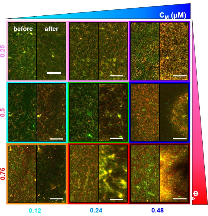
图2双色共聚焦成像观察肌球蛋白浓度不同的肌球蛋白驱动细胞骨架复合物 cM 以及摩尔肌动蛋白组分 ΦA. (A) 256 × 128 方像素(212 × 106 μm2双色共聚焦显微镜图像显示了肌动蛋白纤维(绿色)和微管(红色)复合物的重排方式 通过 肌球蛋白马达活性。不存在驱动蛋白马达或被动交联分子。每个图中,分别显示了肌球蛋白激活45分钟开始时(左,激活前)和结束时(右,激活后)的图像。通过 用488 nm光线照射以使blebbistatin失活)的结果如图所示。各图按肌球蛋白摩尔浓度递增顺序排列。cM),从左到右,肌动蛋白的摩尔分数逐渐增加(ΦA),自上而下排列。每个面板的轮廓颜色与图中使用的颜色编码相对应 图4 和 图5. 比例尺为 50 μM. 为最佳地捕捉用于分析的动态和结构,我们采用 1-5 fps 的帧率,以及包含 50-250 µm 侧面以及5-45分钟的时间序列持续时间,具体取决于收缩和重排的速率。前后图像相似的图示表明结构变化极小,如粉红色、品红色和青色图示所示。小尺度聚集表现为异质性增加以及出现明亮的点状特征,可见于橙色、绿色和红色图示。大尺度收缩表现为网络均匀缩小,明显见于蓝色和紫色图示。该图已根据参考文献修改17. 请点击此处以查看此图的放大版本。

图3粒子图像测速技术(PIV)显示,肌动球蛋白活性可触发共缠结复合物中微丝与微管的协调性收缩动力学。 肌球蛋白驱动的复合体系中肌动蛋白(上排)和微管(下排)的PIV流场ΦA, cM) = (0.5, 0.24) 在6分钟时间序列中随时间递增。流场通过Fiji/ImageJ的PIV插件生成,滞后时间为20 s,空间分辨率为2像素×2像素。在整个视频时长中,肌动蛋白和微管均表现出持续向视野中心区域移动的趋势。所有图像中的比例尺为 50 μm不同箭头颜色对应不同的速度,具体含义参见矢量场右侧的颜色标尺。本图已根据参考文献修改。26. 请点击此处以查看此图的放大版本。
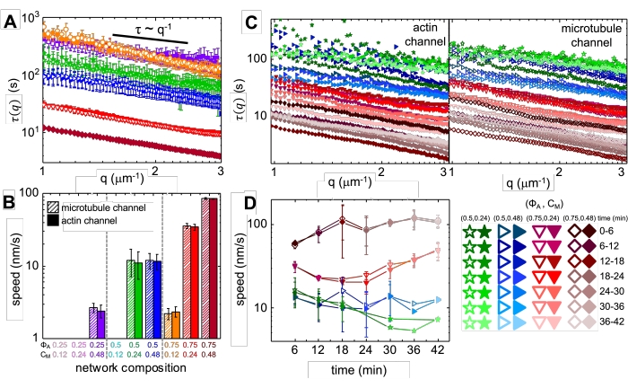
图4时间分辨差分动态显微术(DDM)用于测量活性复合物中肌动蛋白和微管的运动速率与运动类型。 (A对时间序列的微管(上图,空心符号)和肌动蛋白(下图,实心符号)通道进行去相关分析(DDM),以确定其特征衰减时间 τ 波数对比 q 对于肌动蛋白(实心符号)和微管蛋白(空心符号)的处理均如前所述17,26所有曲线均遵循 τ ~ q-1 标度,表明弹道运动,具有速度 v 所确定的 通过 拟合到 τ(q) = (vq)-1. 更快的速度对应更小的 τ(q) 任何给定值的 q符号的颜色和形状对应于(ΦA, cM) B 中所示的组合。B) 收缩速度 v 被确定 通过 拟合到 τ(q) A图中所示曲线为每段45分钟时间序列内所有滞后时间的平均值。 (C时间分辨差分动态显微技术(trDDM)通过评估动力学随时间的变化来量化其动态特性 τ(q) 用于在45分钟激活时间内,连续6分钟间隔(以相同颜色的不同深浅表示)的肌动蛋白(实心符号,左侧)和微管蛋白(空心符号,右侧)。每组均进行trDDM分析。ΦA, cM)组合(如右下角图例中不同符号和颜色所示)。 τ(q) C 中所示曲线与 A 中的曲线遵循相似的缩放规律和趋势,但也显示出某些条件下的时间依赖性ΦA, cM)组成,尤其是对于 ΦA = 0.75. (D) 通过拟合确定肌动蛋白丝(实心符号)和微管(空心符号)的收缩速度 τ(q)曲线。所有图表中的误差线表示三次至五次重复实验值的标准误差。本图改编自参考文献17. 请点击此处以查看此图的放大版本。
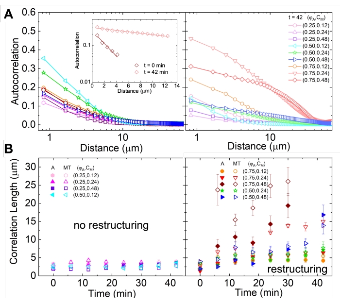
图5空间图像自相关(SIA)分析可量化由马达蛋白驱动的活性细胞骨架复合物的重构过程。 (A自相关 g(r) 实验开始时(左,t = 0 min,深色)和结束时(右,t = 42 min,浅色)的微管ΦA, cM)配方,具体见图注。插图:数据拟合示例  在初始和最终时间点对于(ΦA, cM) = (0.75, 0.12). (B平均相关长度 ξ 用于每组的肌动蛋白(闭合符号)和微管(开放符号)ΦA, cM确定 通过 每个的指数拟合 g(r) 曲线,如A图插图所示。数据被分为表现出最小(左)和显著(右)重构的两组。A和B中的误差条表示三次至五次重复实验的标准误差。该图已根据参考文献修改17. 请点击此处以查看此图的放大版本。
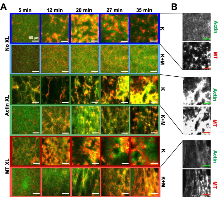
图6将驱动蛋白马达和被动交联剂整合到活性复合材料中,以提高可编程性并拓展其动力学与结构的相空间。 (A活性复合物中肌动蛋白(绿色)和微管(红色)的双色共聚焦图像显示了随时间(以分钟计)变化的复杂且依赖于配方的重构过程。每行中的五幅图像对应于由驱动蛋白(K,第1、3、5行)或驱动蛋白与肌球蛋白(K+M,第2、4、6行)驱动的复合物所采集的2000帧时间序列中的五个帧,且分别不含被动交联剂(无XL,第1、2行)、含有肌动蛋白-肌动蛋白交联(肌动蛋白XL,第3、4行)或微管-微管交联(MT XL,第5、6行)。比例尺均为 50 µm. 轮廓颜色与图中配色方案一致 图8. (B) 仅含驱动蛋白的复合物中,肌动蛋白和微管荧光通道分离显示了多种结构,既有肌动蛋白-微管共定位,也存在微相分离。所示图像为含有 cA = 2.32 μM, cT = 3.48 μM, cK = 0.35 μM, cM = 0.47 μM (第2、4、6行) RA = 0.02(第3、4行),以及 RMT = 0.005(第5、6行)。所有复合物均以均匀分布的肌动蛋白与微管相互贯穿网络为初始状态(第1列)。无交联剂的驱动蛋白驱动复合物(第1行)形成松散连接、富含微管的无定形簇;肌动蛋白最初共定位于这些聚集体的中心,但随后被挤出持续收缩并相互分离的富含微管区域。肌动蛋白-肌动蛋白交联(第3行)阻碍了这种微尺度下的肌动蛋白-微管分离,取而代之的是富含微管的聚集体相互连接 通过 肌动蛋白长链。肌动蛋白交联还使得肌动蛋白缓慢进入微管富集区域,从而使复合物形成共定位的肌动蛋白与微管簇相互连接的网络结构。微管交联(第5行)导致微管无定形聚集并随时间合并,引起肌动蛋白与微管更大尺度的相分离。加入肌球蛋白(第2、4、6行)可减弱驱动蛋白介导的分离与重构。在无交联剂时(第2行),复合物在数小时内几乎不发生重排。交联作用增强了肌动蛋白与微管的重构及共定位(第4、6行)。具体而言,当微管被交联时(第6行),纤维网络显著相互渗透并重组为网状结构。该图已根据参考文献修改50. 请点击此处以查看此图的放大版本。
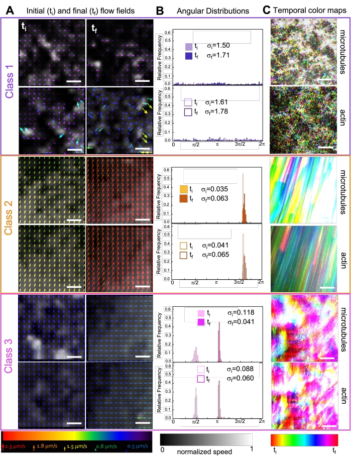
图7PIV 显示,活性复合材料表现出三类在时空上截然不同的流场。 (A第一组PIV流场ti)和最后(tf三个代表性时间序列的帧,展示了所示复合物的不同动力学类别 图6 展示微管(上)和肌动蛋白(下)的PIV流场,对应于第1类(上,紫色)、第2类(中,橙色)和第3类(下,洋红色)示例视频,箭头颜色对应底部的通用速度标尺,灰度 colormap 显示空间速度分布,每个流场根据底部所示标尺单独归一化。比例尺均为 50 μM. (BA点速度矢量的角度分布(以弧度为单位),列出初始和最终的标准差 σi 和 σf. (C) A和B中分析的视频的时间色图显示了每个像素相对于其起始位置的帧间位移。第1类色图显示小尺度的随机运动;第2类色图描绘快速的单向运动,空间或时间变异极小;第3类色图表现出第1类和第2类的特征。该图已根据参考文献修改50. 请点击此处以查看此图的放大版本。
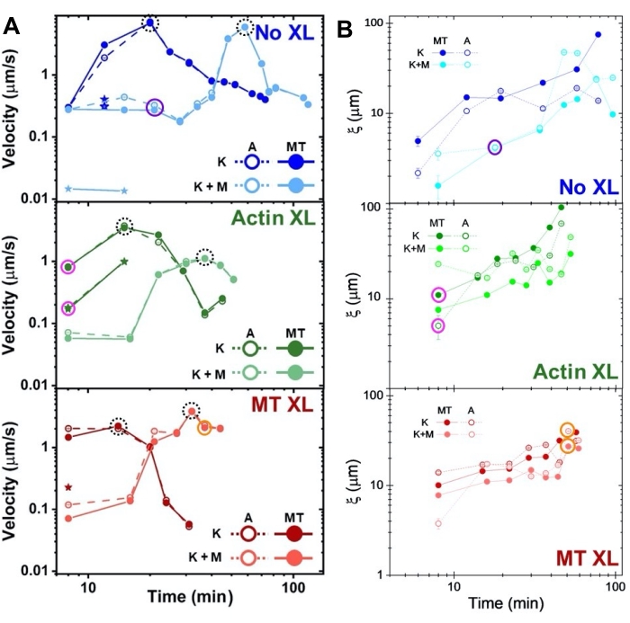
图8DDM 和 SIA 用于测量双马达肌动蛋白-微管复合物随时间变化的动力学与结构。 (A) 所述复合材料的转速 图6 和 图7,测量 通过 DDM,通过交联和肌球蛋白活性编程,展示复合物的加速与减速。在无交联(顶部,蓝色)、肌动蛋白交联(中部,绿色)、微管交联(底部,红色)的复合物中,分别绘制了无肌球蛋白(K,深色)和含肌球蛋白(K+M,浅色)条件下微管(MT,实心圆)和肌动蛋白(A,空心圆)的速度随活性时间的变化曲线。对于具有两种速度的第3类情况,较慢速度以星号标示。由黑色虚线圆圈标出的数据点对应最大速度。 v最大 每种配方的误差棒(多数过小而难以看清)为相应幂律拟合的标准误差 τ(q). (B结构相关长度 ξ,测定 通过 SIA 与活动时间的关系,针对与 A 中相同的时序数据集。每个数据点是相应时序数据第一帧和最后一帧相关长度的平均值。总体而言, ξ 在所有复合体系中,肌动蛋白和微管的相关长度均随时间增加,而仅由驱动蛋白驱动的复合体系比同时含有肌球蛋白的复合体系具有更长的相关长度。A 和 B 中的数据点对应于所分析的三条时间序列。 图7 用相应类别的颜色标出(1 = 紫色,2 = 橙色,3 = 洋红色)。该图已根据参考文献修改50. 请点击此处查看该图的放大版本。
讨论
上述重建系统的一个重要进展在于其模块化和可调性,因此鼓励用户根据预期目标调整蛋白质、马达蛋白、交联分子等组分的浓度,无论是为了模拟特定的细胞过程,还是为了构建具有特定功能或力学性能的材料。肌动蛋白和微管蛋白的浓度范围受限于其聚合所需的临界浓度下限(肌动蛋白约为0.2 μM)57,58,59 和微管蛋白(约为3 - 4 μM)60,以及上限由肌动蛋白丝向向列相排列转变(约90 μM)61,62 或微管(约35 μM)63 所决定。肌动蛋白单体和微管蛋白二聚体应共同聚合形成纤维,而不是在各自聚合后再混合,以确保形成均匀互穿的渗流网络,从而实现协同支撑。复合物所表现出的新颖动力学行为依赖于这种相互作用。虽然为成功重现文中所示结果,通常需要严格按照方案中列出的所有步骤操作,但其中某些步骤要求更为严格,而另一些步骤则可根据具体需求和可用资源进行适当修改和调整。
例如,确保实验结果可重复的一个重要步骤是按照材料表中提供的指南正确配制和储存试剂。细胞骨架蛋白(如肌动蛋白、微管蛋白、肌球蛋白、驱动蛋白)性质不稳定,应分装后用液氮速冻,并在 -80 °C 下以单次使用量分装保存。一旦从 -80 °C 取出,分装样品应始终保持在冰上。细胞骨架蛋白在经历额外的冻融循环后,其功能无法可靠保持。
微管比肌动蛋白对去聚合和变性更为敏感。微管蛋白从 -80 °C 取出后,应在聚合前始终保持在冰上,并在 12 小时内使用。一旦聚合完成,微管应保存在室温下。使用紫杉醇稳定微管以防止其去聚合也至关重要。同样,用鬼笔环肽稳定肌动蛋白纤维对于抑制消耗 ATP 的肌动蛋白踏车现象非常重要,因为该过程会与肌球蛋白和驱动蛋白的活性相竞争。
肌球蛋白马达的超速离心是另一个关键步骤,因为它可以去除无活性的肌球蛋白“死头”。若不除去这些无酶活性的单体,会导致肌动蛋白网络发生被动交联并丧失活性。为了延长马达的ATP酶活性,可加入ATP再生系统,例如磷酸肌酸和磷酸肌酸激酶64。
最后,维持复合体活性需要抑制微丝和马达蛋白在样品腔壁上的吸附,这可以通过对显微镜盖玻片和载玻片进行钝化处理来实现。马达蛋白尤其容易发生吸附,导致复合体被拉向样品腔表面,移出视野范围,塌陷为二维结构,并不再表现出活性。对盖玻片和载玻片进行硅烷化是一种有效的表面钝化方法,可防止吸附(见步骤1)。另一种被有效使用的钝化方法是 体外 细胞骨架实验中的一种方法是用脂质双层包被表面,类似于细胞膜18该方法的优势在于,若希望将蛋白质固定在表面或引入其他特定的蛋白质-表面相互作用,可通过功能化脂双层实现。对于光镊实验而言,微球的钝化同样至关重要,可通过以牛血清白蛋白(BSA)或聚乙二醇(PEG)包被羧基化微球来实现。 通过 碳二亚胺交联化学48.
研究人员可根据需要考虑对本方案中的某些方面进行调整。首先,研究人员可选择用生物来源的交联剂(如分别交联肌动蛋白和微管的α-辅肌动蛋白或MAP65)替代非天然的生物素-NA交联剂。28,65,66使用非天然交联剂是出于其相较于天然交联剂在可重复性、稳定性和可调控性方面的显著优势。由于生物素与链霉亲和素(biotin-NA)之间具有极强的结合力,可认为此类交联剂是永久性的,而大多数天然交联剂则为瞬时结合,且解离速率差异较大。瞬时交联的动力学特性使得解析交联剂与分子马达对系统动力学各自贡献的过程变得复杂。此外,生物素-链霉亲和素交联系统可灵活用于微丝与微管各自的同源交联,也可实现微丝与微管之间的异源交联。因此,在保持其他所有变量(如交联剂尺寸、结合亲和力、化学计量比等)恒定的条件下,能够对不同交联模式进行明确的比较。最后,引入生物素-链霉亲和素交联所需的试剂 commercially available 广泛、特性明确,且已在众多生物物理实验室中普遍使用。然而,该方法的一个关键优势在于 体外 此处所述平台的模块化特性使其具有灵活性,因此研究人员可根据需要无缝地将生物素-NA连接子替换为天然连接子。
其次,在当前的实验方案中,肌动蛋白单体和微管蛋白二聚体在加入样品室之前,先在离心管中共同聚合形成纤维。将缠结的纤维状蛋白质溶液注入样品室时,可能会引起流动取向,尤其是微管的取向,从而破坏复合物所期望的各向同性和均匀性。事实上,以往在稳态肌动蛋白-微管复合物研究中的一个重要进展,是能够在样品室内(in situ)共聚合肌动蛋白和微管,以确保形成各向同性的相互贯穿网络结构15,16,27。然而,将该方法扩展至活性复合物时,需要在肌动蛋白和微管蛋白聚合之前就将马达蛋白加入样品中,并在整个样品于37 °C条件下孵育后再进行实验。对该方案变体的测试结果显示,肌动蛋白的聚合程度降低,且未观察到明显的马达蛋白活性,这可能是由于马达蛋白存在竞争性ATP酶活性以及在37 °C长时间孵育所致。幸运的是,采用当前方案时,并未观察到复合物存在明显的流动取向现象,这一点可以从图2、图3和图6中看出。尽管如此,仍鼓励研究人员设计能够实现活性复合物原位(in situ)形成的实验方案。
另一个需要考虑的问题是荧光标记方案,该方案涉及对网络中所有肌动蛋白丝和微管进行稀疏标记。这种标记方法经过优化,旨在直接观察网络结构,而非通过推断来获取结构与动态信息 通过 示踪细丝或微球。然而,其权衡在于单个细丝的标记较弱且难以分辨。研究人员可采用的一种兼顾单根细丝分辨与网络结构可视化的策略是掺入预先形成的、用另一种荧光染料标记的细丝,从而实现对周围网络结构和单根细丝的同时成像。然而,当使用两种以上的荧光染料及激发/发射通道时,通道间的串扰通常难以完全消除,因此在选择荧光染料、滤光片和激光强度时必须格外谨慎。
另一个局限性在于无法对复合物中的肌球蛋白或驱动蛋白马达进行可视化观察。实验所用的荧光标记肌动蛋白单体和微管蛋白二聚体均为商业化产品,而对复合物中的肌球蛋白或驱动蛋白进行可视化则需要自行标记。建议研究人员进一步开展马达蛋白的标记工作,正如先前研究所实现的那样18,67,以便明确将马达蛋白的活性和结合行为与本研究中复合物所表现出的动力学特征及结构变化直接关联起来。
最后需要指出的是,在本实验方案中,驱动蛋白活性的起始时间和持续时间无法控制。由于如上所述,肌球蛋白活性是通过光去活化blebbistatin来调控的,因此若要实现对驱动蛋白类似的光激活控制,可采用光激活ATP。
为了增加本文所述设计的复杂性,以更好地模拟细胞环境并拓展动态结构-功能参数空间,未来的研究将致力于引入中间纤维(如波形蛋白68,69)以及其他分子马达(如动力蛋白13,70)。此外,还将引入不同浓度的凝溶胶蛋白以调控肌动蛋白的长度14,以及tau蛋白以调控微管的刚度。
综上所述,本文所述的实验方案介绍了如何设计、构建并表征包含两种独立的、可在单一系统内作用于不同底物的活性力生成组分的细胞骨架仿生活性物质系统的动力学、结构与力学特性。这一可调节且模块化的平台使重建工作在模拟细胞骨架方面向前迈出了重要一步,并提供了通过独立地添加、移除或调节不同组分,在宽广的相空间内编程系统特性的独特能力。此外,该多功能系统的全部组分均可通过商业途径获得(参见材料表),唯独驱动蛋白二聚体需在Ross实验室进行纯化,其方法如前所述50,并可根据需求提供。最后,所有分析代码均可通过GitHub免费获取49,且基于开源编程语言与软件(Python和Fiji)。这些系统设计方法的透明化传播,有望使该平台更易于被具有不同专业背景、研究目标、机构归属的广大用户群体所使用。
披露
作者无任何利益冲突需要披露
致谢
我们感谢Maya Hendija和Jonathan Michel博士在数据分析方面提供的帮助,感谢Janet Sheung博士、Moumita Das博士和Michael Rust博士提供的有益讨论与指导。本研究得到了授予RMRA和JLR的威廉·M·凯克基金会研究资助以及美国国家科学基金会DMREF奖(DMR 2119663),以及授予RMR-A和RJM的美国国立卫生研究院R15资助(R15GM123420,2R15GM123420-02)的支持。
材料
| 姓名 | 公司 | 目录编号 | 评论 |
|---|---|---|---|
| (-)-Blebbistatin 论文中使用的缩写: blebbistatin | Sigma Aldrich | B0560 | 储存液浓度: 200 μM 在DMSO中 储存: 干燥,DMSO中,-20ºC 储备液与实验配方: 将1 mg粉末溶解于 200 μM 在DMSO中 储存、操作与故障排除注意事项: 保质期有限,通常在3至4个月后便无法稳定发挥作用。建议每3个月购买并配制新溶液。 |
| 1:20 488-微管蛋白:微管蛋白混合物 论文中使用的缩写: 5-488-微管蛋白 | NA | NA | 储存液浓度: 5 mg/ml,溶于 PEM 储存: 单次使用分装,-80ºC,避免冻融循环 储备液与实验配方: 将微管蛋白与488标记的微管蛋白按20:1的比例混合,用液氮速冻 储存、操作与故障排除注意事项: 每份等分试样在4℃冰上保存时,最长可使用12小时º避光保护 |
| 1:20 R-微管蛋白:微管蛋白混合物 论文中使用的缩写: 5-R-微管蛋白 | NA | NA | 储存液浓度: 5 mg/ml,溶于 PEM 储存: 单次使用分装,-80ºC,避免冻融循环 储备液与实验配方: 将微管蛋白与罗丹明标记的微管蛋白按20:1的比例混合,用液氮速冻 储存、操作与故障排除注意事项: 每份等分试样置于冰上4℃保存时,最多可使用12小时º避光保护 |
| 肌动蛋白(生物素标记):骨骼肌 论文中使用的缩写: 生物素-肌动蛋白 | 细胞骨架 | AB07 | 储存浓度: 1 mg/ml,溶于G缓冲液 储存: 单次使用分装,-80ºC,避免冻融循环 储备液与实验配方: 用G缓冲液重悬至1 mg/ml,液氮速冻 储存、操作与故障排除注意事项: (1) 使用前立即用 PEM 稀释至 0.5 mg/ml,(2) 一旦从 -80℃ 取出ºC,储存 4℃冰上分装ºC,最长可保存1周 |
| 肌动蛋白(罗丹明标记):兔骨骼肌 论文中使用的缩写: R-肌动蛋白 | 细胞骨架 | AR05 | 储存液浓度: 1.5 mg/ml,溶于G缓冲液 储存: 单次使用分装,-80ºC,避免冻融循环 储备液与实验配方: 用G缓冲液重悬至1.5 mg/ml,液氮速冻 储存、操作与故障排除注意事项: 一旦从 -80 取出ºC,储存 4℃冰上分装ºC,最多可使用1周 |
| 三磷酸腺苷 论文中使用的缩写: ATP | 赛默飞世尔科技 | A1048 | 储存液浓度: 100 mM 储存: 在溶液中(pH 7),-20ºC 储备液与实验配方: 用去离子水重悬20,用 NaOH 调节 pH 至 7 储存、操作与故障排除注意事项: 定期检查 pH 值并根据需要进行调整,该溶液会随时间水解,每约 6–12 个月更换一次 |
| AlexaFluor488 Phalloidin 论文中使用的缩写: 488-鬼笔环肽 | 赛默飞世尔科技 | A12379 | 储存液浓度: 100 μM DMSO 储存: 避光,干燥,-20ºC 储备液与实验配方: 重悬至 100 μM 用DMSO处理 储存、操作与故障排除注意事项: 使用前立即稀释至 20 μM 在 PEM 中1 μL 在 4 μL 质子交换膜(PEM) |
| AlexaFluor488–标记的肌动蛋白 论文中使用的缩写: 488-肌动蛋白 | 赛默飞世尔科技 | A12373 | 储存液浓度: 1.5 mg/ml,溶于G缓冲液 储存: 单次使用分装,-80ºC,避免冻融循环 储备液与实验配方: 用G缓冲液重悬至1.5 mg/ml,液氮速冻 储存、操作与故障排除注意事项: 此产品已停产 |
| 基础等离子清洗仪 论文中使用的缩写: 等离子清洗机 | Harrick Plasma | PDC-32G | |
| 贝米斯 Parafilm M 实验室封口膜 论文中使用的缩写: 透明薄膜 | 赛默飞世尔科技 | 13-374-5 | |
| D-(+)-葡萄糖 论文中使用的缩写: | 赛默飞世尔科技 | A1682836 | 储存液浓度: 100x 储存: 于 -20 °C 干燥条件下保存,储存浓度为原液浓度(100 倍)或 10 倍浓度ºC 储备液与实验配方: 将粉末用去离子水重悬至 4.5 mg/ml20 储存、操作与故障排除注意事项: 溶液中的终浓度应 45 μg/mL |
| D-生物素 论文中使用的缩写: 生物素 | Fisher Scientific | BP232-1 | 储存液浓度: 1.02 mM 在 PEM 中 储存: 干燥,4ºC |
| 去离子纳米纯水 论文中使用的缩写: DI | |||
| 二甲基二氯硅烷 论文中使用的缩写: 硅烷 | 赛默飞世尔科技 | D/3820/PB05 | 储存液浓度: 2% 溶于甲苯 |
| 二硫苏糖醇 论文中使用的缩写: DTT | 赛默飞世尔科技 | R0861 | 储存液浓度: 1 M in DMSO 储存: 干燥,-20ºC 储备液与实验配方: 每次实验前用 PEM 立即稀释至 2 mM |
| DMSO 无水 论文中使用的缩写: DMSO | 赛默飞世尔科技 | D12345 | |
| F-缓冲液 论文中使用的缩写: F缓冲液 | NA | NA | 储存液浓度: 10x 储存: 干燥,-20ºC 储备液与实验配方: 10 mM 咪唑(pH 7.0),50 mM KCl,1 mM MgCl₂2,1 mM EGTA,0.2 mM ATP |
| G-缓冲液 论文中使用的缩写: G缓冲液 | NA | NA | 储存浓度: 10x 储存: 干燥,-20ºC 储备液与实验配方: 2.0 mM Tris (pH 8), 0.2 mM ATP, 0.5 mM DTT, 0.1 mM CaCl₂2. 储存于 -20°C. |
| 玻璃显微镜载玻片 论文中使用的缩写: 载玻片 | 赛默飞世尔科技 | 22-310397 | |
| 葡萄糖氧化酶 + 过氧化氢酶 + β-巯基乙醇 论文中使用的缩写: GOC | Sigma Aldrich | G2133-250KU, C1345, 63689 | 储存液浓度: 100x 储存: -20℃干燥保存,储存浓度(100倍浓缩液)或10倍浓缩液ºC 储备液与实验配方: 100倍浓度:4.3 mg/ml 葡萄糖氧化酶,0.7 mg/ml 过氧化氢酶,0.5% v/v β-巯基乙醇在去离子水(DI H₂O)中20 储存、操作与故障排除注意事项: 溶液中的终浓度应为:0.005% β-巯基乙醇, 43 μg/mL 葡萄糖氧化酶 7 μg/mL 过氧化氢酶 |
| 谷氨酸-谷氨酰胺氧化还原循环氧清除系统 论文中使用的缩写: 谷氨酸-草酰乙酸转氨酶 | NA | NA | 储存浓度: 100x 储存: 每次使用时新鲜配制 储备液与实验配方: 等量混合谷氨酸(Glu)和GOC,成像前立即加入,终体积为样品体积的1/100 储存、操作与故障排除注意事项: 成像前立即由Glu和GOC配制 |
| 三磷酸鸟苷 论文中使用的缩写: GTP | 赛默飞世尔科技 | R0461 | 储存液浓度: 100 mM 储存: 100 μL -20 保存的等分试样ºC |
| Instant Mix 1分钟环氧树脂胶 论文中使用的缩写: 环氧树脂 | Loctite | 1366072 | |
| Kinesin-1 401 BIO 6x HIS 论文中使用的缩写: 驱动蛋白 | 在美国雪城大学JL Ross实验室制备 | NA | 储存液浓度: 8.87 μM 在 PEM 中 储存: 单次使用分装,-80ºC,避免冻融循环 储存、操作与故障排除注意事项: 生物素化二聚体形成驱动蛋白簇,每份样品在4℃冰浴中储存可使用长达12小时ºC |
| NeutrAvidin 论文中使用的缩写: NA | 赛默飞世尔科技 | 31000 | 储存浓度: 5 mg/ml,溶于 PEM 储存: 干燥,-20ºC 储备液与实验配方: 将粉末用 PEM 重悬至 5 mg/ml |
| 1 号盖玻片(24 mm × 24 mm) 论文中使用的缩写: 盖玻片 | 赛默飞世尔科技 | 12-548-CP | |
| 紫杉醇 论文中使用的缩写: 紫杉醇 | 赛默飞世尔科技 | P3456 | 储存液浓度: 2 mM DMSO溶液 储存: 避光,干燥,-20ºC 储备液与实验配方: 用DMSO重悬至2 mM 储存、操作与故障排除注意事项: 使用前立即稀释至 200 μM 在 DMSO 中(0.4 μL 在 3.6 μL DMSO |
| PEM-100 论文中使用的缩写: PEM | NA | NA | 储存液浓度: 1x 储存: 室温(RT) 储备液与实验配方: 100 mM K-PIPES(pH 6.8),2 mM EGTA,2 mM MgCl₂2 储存、操作与故障排除注意事项: 使用KOH调节pH至6.8,频繁重新检测pH并相应调整 |
| 鬼笔环肽 论文中使用的缩写: 鬼笔环肽 | 赛默飞世尔科技 | P3457 | 储存浓度: 100 μM 在DMSO中 储存: 避光,干燥,-20ºC,严格遵守储存和操作条件 储备液与实验配方: 重悬至 100 μM 用DMSO处理 储存、操作与故障排除注意事项: 易受制备过程中的杂质及变性影响,表现为样品中可识别出的大块无定形肌动蛋白聚集体 |
| 猪脑微管蛋白 论文中使用的缩写: 微管蛋白 | 细胞骨架 | T240 | 储存液浓度: 5 mg/ml,溶于 PEM 储存: 单次使用分装,-80ºC,避免冻融循环 储备液与实验配方: 用 PEM 将粉末重悬至 5 mg/ml,液氮速冻 储存、操作与故障排除注意事项: 每份等分试样在4℃冰上保存时,最多可使用12小时ºC |
| 氯化钾 论文中使用的缩写: KCl | 赛默飞世尔科技 | AM9640G | 储存液浓度: 4 M 储存: RT |
| 兔骨骼肌动蛋白 论文中使用的缩写: 肌动蛋白 | 细胞骨架 | AKL99 | 储存液浓度: 2 mg/ml,溶于G缓冲液 储存: 单次使用分装,-80ºC,避免冻融循环 储备液与实验配方: 用G缓冲液重悬至2 mg/ml,液氮速冻 储存、操作与故障排除注意事项: 一旦从 -80 取出ºC,储存 4℃冰上分装ºC,最多可使用1周 |
| 兔骨骼肌肌球蛋白 II 论文中使用的缩写: 肌球蛋白 | 细胞骨架 | MY02 | 储存浓度: 10 mg/ml,溶于 PEM 储存: 单次使用分装,-80ºC,避免冻融循环 储备液与实验配方: 用 PEM 将粉末重悬至 10 mg/ml,液氮速冻 储存、操作与故障排除注意事项: 单体在低浓度KCl条件下形成微丝,每份样品在4℃冰上保存可使用长达12小时ºC |
| 微管蛋白(生物素标记):猪脑 论文中使用的缩写: 生物素-微管蛋白 | 细胞骨架 | T333P | 储存浓度: 5 mg/ml,溶于 PEM 储存: 单次使用分装,-80ºC,避免冻融循环 储备液与实验配方: 用 PEM 将粉末重悬至 5 mg/ml,液氮速冻 储存、操作与故障排除注意事项: 使用前立即用 PEM 稀释至 0.5 mg/ml |
| 微管蛋白(荧光HiLyte 488标记):猪脑来源 论文中使用的缩写: 488-微管蛋白 | 细胞骨架 | TL488M | 储存液浓度: 5 mg/ml,溶于 PEM 储存: 单次使用分装,-80ºC,避免冻融循环 储备液与实验配方: 用 PEM 将粉末重悬至 5 mg/ml,液氮速冻 储存、操作与故障排除注意事项: 每份等分试样在4℃冰浴中储存可使用长达12小时ºC,避光保护 |
| 微管蛋白(罗丹明标记):猪脑 论文中使用的缩写: R-tubulin | 细胞骨架 | TL590M | 储存液浓度: 5 mg/ml,溶于 PEM 储存: 单次使用分装,-80ºC,避免冻融循环 储备液与实验配方: 用 PEM 将粉末重悬至 5 mg/ml,液氮速冻 储存、操作与故障排除注意事项: 每份等分试样在4℃冰上保存时最多可使用12小时ºC,避光保护 |
| Tween 20 论文中使用的缩写: Tween20 | 赛默飞世尔科技 | J20605.AP | 储存浓度: 1% v/v,溶于去离子水20 储存: RT |
| 超速离心级微量离心管 论文中使用的缩写: 贝克曼库尔特 Optima Max XP | 贝克曼库尔特 | 343776 | 储存、操作与故障排除注意事项: 8x34 mm PC |
| 紫外光固化胶 论文中使用的缩写: 紫外胶 | 法尔达 | SKG-2869 |
参考文献
- Fletcher, D. A., Mullins, R. D. Cell mechanics and the cytoskeleton. Nature. 463 (7280), 485-492 (2010).
- Koenderink, G. H., Paluch, E. K. Architecture shapes contractility in actomyosin networks. Current Opinion in Cell Biology. 50, 79-85 (2018).
- Dogterom, M., Koenderink, G. H. Actin-microtubule crosstalk in cell biology. Nature Reviews Molecular Cell Biology. 20 (1), 38-54 (2019).
- Burla, F., Mulla, Y., Vos, B. E., Aufderhorst-Roberts, A., Koenderink, G. H. From mechanical resilience to active material properties in biopolymer networks. Nature Reviews Physics. 1 (4), 249-263 (2019).
- Wen, Q., Janmey, P. A. Polymer physics of the cytoskeleton. Current Opinion in Solid State and Materials Science. 15 (5), 177-182 (2011).
- Xiao, Q., Hu, X., Wei, Z., Tam, K. Y. Cytoskeleton molecular motors: structures and their functions in neuron. International Journal of Biological Sciences. 12 (9), 1083-1092 (2016).
- Ajeti, V. et al. Wound healing coordinates actin architectures to regulate mechanical work. Nature Physics. 15 (7), 696-705 (2019).
- Jung, W. et al. Dynamic motions of molecular motors in the actin cytoskeleton. Cytoskeleton. 76 (11-12), 517-531 (2019).
- Pollard, T. D., O'Shaughnessy, B. Molecular mechanism of cytokinesis. Annual Review of Biochemistry. 88 (1), 661-689 (2019).
- Huber, F., Boire, A., López, M. P., Koenderink, G. H. Cytoskeletal crosstalk: when three different personalities team up. Current Opinion in Cell Biology. 32, 39-47 (2015).
- Rivero, F. et al. The role of the cortical cytoskeleton: F-actin crosslinking proteins protect against osmotic stress, ensure cell size, cell shape and motility, and contribute to phagocytosis and development. Journal of Cell Science. 109 (11), 2679-2691 (1996).
- Duclos, G. et al. Topological structure and dynamics of three-dimensional active nematics. Science. 367 (6482), 1120-1124 (2020).
- Baclayon, M. et al. Optical tweezers-based measurements of forces and dynamics at microtubule ends. Optical Tweezers. 1486, 411-435 (2017).
- Gurmessa, B., Fitzpatrick, R., Falzone, T. T., Robertson-Anderson, R. M. Entanglement density tunes microscale nonlinear response of entangled actin. Macromolecules. 49 (10), 3948-3955 (2016).
- Francis, M. L. et al. Non-monotonic dependence of stiffness on actin crosslinking in cytoskeleton composites. Soft Matter. 15 (44), 9056-9065 (2019).
- Ricketts, S. N. et al. Varying crosslinking motifs drive the mesoscale mechanics of actin-microtubule composites. Scientific Reports. 9 (1), 12831 (2019).
- Lee, G. et al. Active cytoskeletal composites display emergent tunable contractility and restructuring. Soft Matter. 17 (47), 10765-10776 (2021).
- Murrell, M. P., Gardel, M. L. F-actin buckling coordinates contractility and severing in a biomimetic actomyosin cortex. Proceedings of the National Academy of Sciences. 109 (51), 20820-20825 (2012).
- Soares e Silva, M. et al. Active multistage coarsening of actin networks driven by myosin motors. Proceedings of the National Academy of Sciences. 108 (23), 9408-9413 (2011).
- Sonn-Segev, A., Bernheim-Groswasser, A., Roichman, Y. Dynamics in steady state in vitro acto-myosin networks. Journal of Physics: Condensed Matter. 29 (16), 163002 (2017).
- Ideses, Y., Sonn-Segev, A., Roichman, Y., Bernheim-Groswasser, A. Myosin II does it all: assembly, remodeling, and disassembly of actin networks are governed by myosin II activity. Soft Matter. 9 (29), 7127 (2013).
- Fürthauer, S. et al. Self-straining of actively crosslinked microtubule networks. Nature Physics. 15 (12), 1295-1300 (2019).
- Lemma, L. M. et al. Multiscale microtubule dynamics in active nematics. Physical Review Letters. 127 (14), 148001 (2021).
- Fan, Y., Wu, K.-T., Aghvami, S. A., Fraden, S., Breuer, K. S. Effects of confinement on the dynamics and correlation scales in kinesin-microtubule active fluids. Physical Review E. 104 (3), 034601 (2021).
- Triclin, S. et al. Self-repair protects microtubules from destruction by molecular motors. Nature Materials. 20 (6), 883-891 (2021).
- Lee, G. et al. Myosin-driven actin-microtubule networks exhibit self-organized contractile dynamics. Science Advances. 7 (6), eabe4334 (2021).
- Ricketts, S. N., Ross, J. L., Robertson-Anderson, R. M. Co-entangled actin-microtubule composites exhibit tunable stiffness and power-law stress relaxation. Biophysical Journal. 115 (6), 1055-1067 (2018).
- Bendix, P. M. et al. A quantitative analysis of contractility in active cytoskeletal protein networks. Biophysical Journal. 94 (8), 3126-3136 (2008).
- Linsmeier, I. et al. Disordered actomyosin networks are sufficient to produce cooperative and telescopic contractility. Nature Communications. 7 (1), 12615 (2016).
- Stam, S. et al. Filament rigidity and connectivity tune the deformation modes of active biopolymer networks. Proceedings of the National Academy of Sciences. 114 (47), E10037-E10045 (2017).
- Yadav, V. et al. Filament nucleation tunes mechanical memory in active polymer networks. Advanced Functional Materials. 29 (49), 1905243 (2019).
- Ennomani, H. et al. Architecture and connectivity govern actin network contractility. Current Biology. 26 (5), 616-626 (2016).
- Alvarado, J., Sheinman, M., Sharma, A., MacKintosh, F. C., Koenderink, G. H. Molecular motors robustly drive active gels to a critically connected state. Nature Physics. 9 (9), 591-597 (2013).
- Alvarado, J., Cipelletti, L., Koenderink, G. H. Uncovering the dynamic precursors to motor-driven contraction of active gels. Soft Matter. 15 (42), 8552-8565 (2019).
- Jung, W., Murrell, M. P., Kim, T. F-actin cross-linking enhances the stability of force generation in disordered actomyosin networks. Computational Particle Mechanics. 2 (4), 317-327 (2015).
- Lenz, M., Thoresen, T., Gardel, M. L., Dinner, A. R. Contractile units in disordered actomyosin bundles arise from f-actin buckling. Physical Review Letters. 108 (23), 238107 (2012).
- Memarian, F.L. et al. Active nematic order and dynamic lane formation of microtubules driven by membrane-bound diffusing motors. Proceedings of the National Academy of Sciences. 118 (52), e2117107118 (2021).
- Needleman, D., Dogic, Z. Active matter at the interface between materials science and cell biology. Nature Reviews Materials. 2 (9), 17048 (2017).
- Foster, P. J., Fürthauer, S., Shelley, M. J., Needleman, D. J. Active contraction of microtubule networks. eLife. 4, e10837 (2015).
- Thijssen, K. et al. Submersed micropatterned structures control active nematic flow, topology, and concentration. Proceedings of the National Academy of Sciences. 118 (38), e2106038118 (2021).
- Sanchez, T., Chen, D. T. N., DeCamp, S. J., Heymann, M., Dogic, Z. Spontaneous motion in hierarchically assembled active matter. Nature. 491 (7424), 431-434 (2012).
- Colen, J. et al. Machine learning active-nematic hydrodynamics. Proceedings of the National Academy of Sciences. 118 (10), e2016708118 (2021).
- Mitchell, K. A., Tan, A. J., Arteaga, J., Hirst, L. S. Fractal generation in a two-dimensional active-nematic fluid. Chaos: An Interdisciplinary Journal of Nonlinear Science. 31 (7), 073125 (2021).
- Pandolfi, R. J., Edwards, L., Johnston, D., Becich, P., Hirst, L. S. Designing highly tunable semiflexible filament networks. Physical Review E. 89 (6), 062602 (2014).
- Tan, A. J. et al. Topological chaos in active nematics. Nature Physics. 15 (10), 1033-1039 (2019).
- Roostalu, J., Rickman, J., Thomas, C., Nédélec, F., Surrey, T. Determinants of polar versus nematic organization in networks of dynamic microtubules and mitotic motors. Cell. 175 (3), 796-808.e14 (2018).
- Ndlec, F. J., Surrey, T., Maggs, A. C., Leibler, S. Self-organization of microtubules and motors. Nature. 389 (6648), 305-308 (1997).
- Sheung, J. Y. et al. Motor-driven restructuring of cytoskeleton composites leads to tunable time-varying elasticity. ACS Macro Letters. 10 (9), 1151-1158 (2021).
- McGorty, R. PyDDM v0.2.0. Zenodo. (2022).
- Achiriloaie, D. H. et al. Kinesin and myosin motors compete to drive rich multi-phase dynamics in programmable cytoskeletal composites. arXiv. (2021).
- Wulstein, D. M., Regan, K. E., Garamella, J., McGorty, R. J., Robertson-Anderson, R. M. Topology-dependent anomalous dynamics of ring and linear DNA are sensitive to cytoskeleton crosslinking. Science Advances. 5 (12), eaay5912 (2019).
- McGorty, R. Image-Correlation. at <https://github.com/rmcgorty/Image-Correlation>. (2020).
- Robertson, C. Theory and practical recommendations for autocorrelation-based image correlation spectroscopy. Journal of Biomedical Optics. 17 (8), 080801 (2012).
- McGorty, R. Differential Dynamic Microscopy - Python. at <https://github.com/rmcgorty/Differential-Dynamic-Microscopy---Python>. (2021).
- Cerbino, R., Trappe, V. Differential dynamic microscopy: probing wave vector dependent dynamics with a microscope. Physical Review Letters. 100 (18), 188102 (2008).
- Robertson-Anderson, R. M. Optical tweezers microrheology: from the basics to advanced techniques and applications. ACS Macro Letters. 7 (8), 968-975 (2018).
- Pollard, T. D. Polymerization of ADP-actin. Journal of Cell Biology. 99 (3), 769-777 (1984).
- Coué, M., Brenner, S. L., Spector, I., Korn, E. D. Inhibition of actin polymerization by latrunculin A. FEBS Letters. 213 (2), 316-318 (1987).
- Pollard, T. D. Actin and actin-binding proteins. Cold Spring Harbor Perspectives in Biology. 8 (8), a018226 (2016).
- Kumar, N. Taxol-induced polymerization of purified tubulin. Mechanism of action. Journal of Biological Chemistry. 256 (20), 10435-10441 (1981).
- Käs, J. et al. F-actin, a model polymer for semiflexible chains in dilute, semidilute, and liquid crystalline solutions. Biophysical Journal. 70 (2), 609-625 (1996).
- Viamontes, J., Narayanan, S., Sandy, A. R., Tang, J. X. Orientational order parameter of the nematic liquid crystalline phase of F -actin. Physical Review E. 73 (6), 061901 (2006).
- Hitt, A. L., Cross, A. R., Williams, R. C. Microtubule solutions display nematic liquid crystalline structure. Journal of Biological Chemistry. 265 (3), 1639-1647 (1990).
- Andexer, J. N., Richter, M. Emerging enzymes for ATP regeneration in biocatalytic processes. ChemBioChem. 16 (3), 380-386 (2015).
- Farhadi, L. et al. Actin and microtubule crosslinkers tune mobility and control co-localization in a composite cytoskeletal network. Soft Matter. 16 (31), 7191-7201 (2020).
- Falzone, T. T., Lenz, M., Kovar, D. R., Gardel, M. L. Assembly kinetics determine the architecture of α-actinin crosslinked F-actin networks. Nature Communications. 3 (1), 861 (2012).
- Thoresen, T., Lenz, M., Gardel, M. L. Reconstitution of contractile actomyosin bundles. Biophysical Journal. 100 (11), 2698-2705 (2011).
- Sanghvi-Shah, R., Weber, G. F. Intermediate filaments at the junction of mechanotransduction, migration, and development. Frontiers in Cell and Developmental Biology. 5, 81 (2017).
- Shen, Y. et al. Effects of vimentin intermediate filaments on the structure and dynamics of in vitro multicomponent interpenetrating cytoskeletal networks. Physical Review Letters. 127 (10), 108101 (2021).
- Laan, L., Roth, S., Dogterom, M. End-on microtubule-dynein interactions and pulling-based positioning of microtubule organizing centers. Cell Cycle. 11 (20), 3750-3757 (2012).
重印与许可
勘误
Formal Correction: Erratum: Reconstituting and Characterizing Actin-Microtubule Composites with Tunable Motor-Driven Dynamics and Mechanics
Posted by JoVE Editors on 10/11/2022. Citeable Link.
An erratum was issued for: Reconstituting and Characterizing Actin-Microtubule Composites with Tunable Motor-Driven Dynamics and Mechanics. The Authors section was updated.
Mehrzad Sasanpour1
Daisy H. Achiriloaie1,2
Gloria Lee1
Gregor Leech1
Christopher Currie1
K. Alice Lindsay3
Jennifer L. Ross3
Ryan J. McGorty1
Rae M. Robertson-Anderson1
1Department of Physics and Biophysics, University of San Diego
2W. M. Keck Science Department, Scripps College, Pitzer College, and Claremont McKenna College
3Department of Physics, Syracuse University
to:
Mehrzad Sasanpour1
Daisy H. Achiriloaie1,2
Gloria Lee1
Gregor Leech1
Maya Hendija1
K. Alice Lindsay3
Jennifer L. Ross3
Ryan J. McGorty1
Rae M. Robertson-Anderson1
1Department of Physics and Biophysics, University of San Diego
2W. M. Keck Science Department, Scripps College, Pitzer College, and Claremont McKenna College
3Department of Physics, Syracuse University
