A Hybrid Neutrosophic Deep Learning Framework with Multi-Convolutional Neural Network Feature Fusion for Robust Facial Recognition

摘要

This paper presents a hybrid deep learning framework for robust facial recognition under varying illumination, occlusion, facial expressions, and image noise. The framework fuses deep features extracted from multiple pre-trained convolutional neural networks (CNNs) to enhance recognition accuracy and robustness. Experiments on a small custom dataset demonstrate promising preliminary performance.

摘要

The performance of many facial recognition (FR) algorithms is adversely affected in uncontrolled settings due to diverse facial expressions, lighting changes, occlusions, and image noise. This poses a significant challenge in developing a reliable and accurate facial recognition system for real-world applications. Hence, this paper introduces a novel hybrid deep learning-based facial recognition framework aimed at overcoming the shortcomings of the current solutions, specifically, inaccuracy and poor computational efficiency caused by complex facial images. Several pre-trained CNN architectures (VGG16, EfficientNetB0, ResNet-50, MobileNet, MobileNetV2, Xception, InceptionResNetV2, and NASNetLarge) are utilized in the proposed solution. Eight CNN models were evaluated, and the four most effective were identified based on their performance metrics. The proposed hybrid system employs a feature-level fusion method in which deep features from the best-performing models are combined. Subsequently, a smoothing operation on the resultant feature vector was performed, and the output vector was flattened and concatenated for the classification stage. According to the experimental results, the proposed hybrid framework outperforms all the individual CNN models used in the study, achieving an accuracy rate of 96.9%, a precision of 94.1%, a recall of 100%, and an F1-score of 96.9%.

引言

Traditional human-to-computer authentication is generally divided into three main types: knowledge-based authentication (such as passwords), possession-based authentication (like smartcards), and inherence-based authentication, which makes use of biometrics^1,2. The biometrics used can either be physiological characteristics or behavioral characteristics. Physiological characteristics include features like the face, fingerprints, palm print, ear, and tongue, whereas behavioral characteristics refer to actions performed by users, such as gait and signature^3,4. Examples of these biometric modalities are illustrated in Figure 1.

For biometric systems to be effective, there are some basic requirements that need to be fulfilled. These include characteristics such as collectability, permanence, accuracy, universality, and user acceptance. The registration process needs to be simple, and the biometric traits collected need to be temporally stable. The selected biometric technology should be universal enough to accommodate a wide range of users⁵. Facial recognition is one of the commonly used physiological biometric technologies. The main strengths of the facial recognition technology compared to other biometric techniques lie in its non-invasive nature, simplicity, ease of adoption, and high levels of accuracy⁶. However, the efficiency of face recognition algorithms may be significantly impaired when applied in unconstrained settings due to variations in facial expressions (happy, neutral, or sad faces), occlusions (spectacles, caps, shawls, or masks), and lighting condition variations. A face recognition algorithm involves detecting and comparing specific facial features, such as the distance between eyes, the width of the nose, and the shape of the jaw. Such measurements are encoded into discriminative representations that enable the system to distinguish between different individuals.

A machine learning-based solution for enhancing the efficiency of facial recognition systems has been developed by⁵. In the experimental analysis, the MUCT facial image dataset was used since it provides a variety of facial images under different lighting conditions and includes people from various age groups and ethnicities. For detecting and localizing faces in the images, the Viola–Jones face detection algorithm was used. To address the high dimensionality of the extracted features, linear discriminant analysis (LDA) was performed. These low-dimensional features were classified using some machine learning models, among which decision tree classifiers were preferred due to their transparency in decision-making. According to their experiments, the proposed system achieved promising results regarding recognition accuracy⁷ have examined the ability of four well-known facial analysis tools, Face++ , IBM Bluemix Visual Recognition, AWS Recognition, and Microsoft Azure Face API, to perform different demographic inference tasks using various datasets. According to their obtained results, most tools showed impressive accuracy (>90%) for gender recognition, while the performance of IBM Bluemix was relatively low compared to other tools. As regards race recognition, only one tool, Face++, supported this feature, and its performance was relatively high (>90% accuracy) for high-quality datasets. On the contrary, age prediction appeared to be a challenging task, which could not be successfully completed by any of the four tools. Their experiment shows the differences between the performance of several tools used for analyzing faces depending on the type of task performed.

This study emphasizes the need to choose appropriate tools and verify their performance before implementing them in practical applications, such as computational social science. A study introduced ArcFace, a method for face recognition based on adding angular margin loss into the model architecture to improve discriminative feature learning⁸. One major contribution from the paper concerns the geometric intuition behind ArcFace, in which feature vectors are trained on the hypersphere via geodesic distance. Their experiments included thorough tests on ten public benchmarks, in which their proposed solution outperformed existing methods in terms of accuracy while keeping costs relatively low. The accuracy scores they obtained were reported as 99.82%, 95.45%, and 92.08% for LFW, CALFW, and CPLFW datasets, respectively.

Facial recognition systems usually analyze the dimensions, contours, and geometric relations among some of the important facial landmarks, such as the eyes, nose, and mouth, in addition to other prominent regions of the face. To enhance recognition accuracy, some models utilize dynamic elements like lip and mouth motion in video-based systems. The recognition procedure involves analyzing the unique characteristics of the face from the images or video data, then converting them into numeric codes. Then, the codes are combined into a single code representing the entire face, making it easy to distinguish one person from another⁷. In recent years, the facial recognition algorithm has been enhanced by machine learning and deep learning algorithms^9,10. Figure 2 presents conventional facial recognition pipeline, which typically relies on a single feature extraction model. However, such approaches suffer from limitations, including sensitivity to variations in lighting, occlusion, and the absence of uncertainty modeling, which motivates the proposed framework.

The optimization process takes into consideration several objectives, including maximizing the facial features’ classification, minimizing possible ambiguity in the representation of features, and minimizing the probability of false positives, while also taking into account any indeterminate cases. For this purpose, it can use meta-heuristic optimization techniques such as particle swarm optimization (PSO) and genetic algorithms (GA) to tune the parameters of the proposed neutrosophic-based deep learning model. In this paper, an innovative approach to facial recognition based on deep learning will be designed. The aim of this research is to develop a facial recognition technique for use in a biometric authentication system. As biometric face recognition technology develops rapidly, there is an increased need to apply methodologies that can handle the presence of uncertainties and ambiguities in the process of recognition. Binary classification approaches have proven to be inadequate in many practical applications where unfavorable conditions, such as low illumination, occlusion, and various angles of poses, are present.

The main contributions made by this research were summarized as follows. The authors proposed a hybrid ensemble framework that systematically evaluated and selected the most effective CNN architectures for facial recognition, addressing key challenges posed by lighting changes, occlusion, and other forms of environmental disturbances in uncontrolled conditions. The authors introduced a novel facial recognition framework that combined the top-performing models, EfficientNetB0 and ResNet-50, to address challenges related to accuracy and robustness in real-world authentication scenarios. The authors empirically validated the framework and achieved strong performance results, with an accuracy of 96.9%, precision of 94.1%, recall of 100%, and an F1-score of 96.9%, demonstrating the effectiveness of the proposed framework for real-world authentication applications.

Facial recognition technology has achieved great advances through application of deep learning methods such as convolutional neural networks (CNNs), which have proven to be more effective at learning discriminative facial features than previous methods^11,12. Initially, facial recognition required the utilization of manual or handcrafted features. However, recently, deep learning models have mostly been applied for learning hierarchical representations automatically. Some of the pioneering CNN architectures include VGG16¹³, a deep model with uniform filter size that uses small filters to facilitate better feature learning for large-scale image classification problems¹⁴. ResNet¹⁵ was developed to improve the results of previous models by adding residual connections to solve the vanishing gradient problem and to enable the construction of even deeper models. Inception-type architectures allowed enhancing computational efficiency by using convolutional filters of different sizes in parallel. Further developments of Inception models like InceptionResNetV2¹⁶ enabled learning residual connections in addition to multi-scale filtering.

The lightweight architectures such as MobileNet¹⁷ and MobileNetV2¹⁸ allow efficient computation through the use of depth-wise separable convolutions resulting in parameter reduction without compromising performance. EfficientNet was designed with a compound scaling mechanism that considers three factors: network depth, width, and resolution to achieve superior results. Xception¹⁹ further enhanced CNN operations by employing depth-wise separable convolutions for improved performance using smaller numbers of parameters²⁰. Another type of model employed to train deep facial recognition models is metric learning models. ArcFace²¹ is one such model that utilizes an additive angular margin loss for learning discriminative facial representations^21,22. As a result, the model achieves superior results. However, it has been found that many methods used for training facial recognition models use single-model architectures which make them less flexible and therefore may fail to capture various complex facial features²². Ensemble learning methods have been suggested as a possible solution in this case since they incorporate several models into the design. However, most current approaches focus only on features aggregation without considering uncertainty¹².

The performance of the proposed method was evaluated by testing the extracted facial features using the decision tree (DT), k-nearest neighbor (KNN), and support vector machine (SVM). Evaluation was conducted on the SDUMLAHMT^23,24,25 and CASIA face databases^11,12. The performance of the method was evaluated using criteria such as accuracy, precision, recall, specificity, and processing time in comparison to other methods. The distribution of classes in the original and neutrosophic datasets is given in Table 1. To investigate complementary feature representations, the study evaluates the CNN architectures listed in Table 2. The architectures are first evaluated individually, after which the predefined selection procedure is used to determine which models are included in the final framework. The selected architectures provide complementary deep feature representations that are subsequently investigated through feature-level fusion. The final model configuration is defined explicitly in the Experimental Protocol and is kept consistent throughout the manuscript.

方案

The study was conducted in accordance with the ethical principles and applicable institutional guidelines governing research. The protocol aims to develop a robust facial recognition (FR) system capable of operating under uncontrolled environments, including variations in illumination, facial expressions, occlusion, and noise. The framework integrates multiple deep learning models to enhance recognition accuracy and generalization. All the materials used in this study are available in the Table of Materials.

Data acquisition and preprocessing

Facial image datasets are collected from publicly available or benchmark sources. The preprocessing pipeline includes face detection and cropping, Image resizing to a uniform input size (e.g., 180×180), normalization of pixel values, and data augmentation (rotation, flipping, brightness adjustment) to simulate real-world variability.

Model selection strategy

Initially, eight CNN models are evaluated using standard performance metrics (accuracy, precision, recall, and F1-score). Based on comparative analysis, the top two performing models are selected for hybridization to ensure optimal feature representation and computational balance.

Feature extraction using pre-trained CNN models

Two state-of-the-art pre-trained convolutional neural network (CNN) architectures are employed: EfficientNetB0 and ResNet-50. Each model is fine-tuned on the target dataset using transfer learning. The fully connected classification layers are removed, and deep feature vectors are extracted from the final pooling layers. The proposed framework extracts the feature vectors from the selected models, concatenates them into a unified representation, applies a smoothing operation (e.g., moving average or filtering) to reduce noise and redundancy, and flattens the fused feature vector to create a compact and discriminative representation.

Classification stage

The fused representation is passed to a binary classification layer that determines whether the input image belongs to the enrolled target subject. A sigmoid activation function is used to produce the probability of the positive class, and binary cross-entropy is used as the training loss. A threshold of 0.5 is used to convert the predicted probability into the final binary decision.

Performance evaluation

The system is evaluated using accuracy, precision, recall, and F1-score. Experimental results demonstrate that the hybrid model significantly outperforms individual CNN architectures, achieving Accuracy: 96.9%, Precision: 94.1%, Recall: 100%, and F1-score: 96.9%.

Deployment considerations

The model is designed for real-world deployment with considerations for reduced computational complexity via selective model fusion, Scalability to large datasets, and Robustness under uncontrolled imaging conditions.

结果

Data collection

The custom dataset used in this experiment includes face images of 7 people, taken under free conditions, including changes in lighting, occlusions, and expressions. The images were collected from students at Amman Arab University in Jordan. Although facial recognition can be formulated as either identification or verification depending on the application scenario, the present study considers a binary classification problem. The model determines whether a given facial image belongs to the enrolled target subject (Yes) or not (No). A major shortcoming of this dataset is its small number of images. To alleviate this problem, a technique for generating more data using neutrosophic augmentation was implemented. Table 1 presents the distribution of data classes in the original and neutrosophic datasets across the training and testing sets. In the original dataset, the training set comprised 34 instances labeled Yes and 25 labeled No, while the testing set contained 8 instances for each class, resulting in 75 observations overall. Following the application of the neutrosophic transformation, the dataset size increased to 150 instances, with the training subset containing 68 Yes and 50 No observations, and the testing subset comprising 16 instances from each class. Thus, the transformation effectively doubled the number of observations while preserving the original class proportions and maintaining the same distribution pattern between the training and testing subsets.

Neutrosophic sets

In contrast to classical set theory, neutrosophic sets provide a more sophisticated mathematical apparatus, which takes into account indeterminacy and inconsistency. While binary logic systems represent only two types of membership, the absence or presence of the given element in the set, neutrosophic sets consider additional aspects of uncertainty. Introduced by Florentin Smarandache, this theory describes how uncertainty, inconsistencies, and partial truths can be represented using different parameters^26,27. In contrast to classical fuzzy sets, where the membership is expressed using a single degree within the interval from 0 to 1, neutrosophic sets use three degrees, truth-membership T (x), indeterminacy-membership I(x), and falsity-membership F(x) of the given element x. Each parameter takes values from the interval [0, 1], but the sum of the three degrees is not necessarily equal to 1. This innovative approach creates a convenient mechanism for representing uncertain information. Thus, it can be used for capturing ambiguity and inconsistency in facial recognition when identifying faces and their features. Each facial feature (e.g., the shape of the eye or nose, the contour of the mouth, etc.) can be described by a neutrosophic model. This description will include several degrees of truth, indeterminacy, and falsity. It can be expressed as follows:

N(x) ={T(x),I(x),F(x) }  (1)

where x is a certain facial feature. As a result, all critical data about features can be captured using a single approach. The practical application of neutrosophic sets is demonstrated in numerous areas, including uncertainty-based decision-making, medical image analysis, database systems, pattern recognition, and others. For instance, in image analysis, this approach can be useful for detecting ambiguity in medical images by estimating the levels of truth, indeterminacy, and falsity.

For an input grayscale facial image G(x,y), the neutrosophic transformation represents each pixel using three membership components: truth (T), indeterminacy (I), and falsity (F). The transformation converts the original image into a neutrosophic domain as:

P_NS (x,y) = {T(x,y),I(x,y),F(x,y)}  (2)

where T(x,y),I(x,y), and F(x,y) indicate the degree of belongingness of each pixel to the true, uncertain, and false sets, respectively.

The truth component was calculated based on the normalized intensity value:

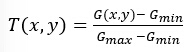 (3)

where G_min​ and G_max​ represent the minimum and maximum intensity values in the input image.

To estimate local uncertainty, the local mean intensity was calculated using a sliding window:

   (4)

where w = 2k + 1 represents the window size. In this study, a 3 × 3 neighborhood window was used (k = 1).

The indeterminacy component was computed according to the local intensity variation:

   (5)

followed by min-max normalization to maintain values within the range [0,1]. The falsity component was obtained as the complementary membership value:

F(x,y) = 1 - T(x,y)  (6)

All three components were independently normalized to the interval [0,1] before being combined to form the neutrosophic representation:

NS(x,y) = [T(x,y),I(x,y),F(x,y) ]  (7)

The resulting neutrosophic image was therefore represented as a three-channel tensor with dimensions equivalent to an RGB image: H×W×3. Where the three channels correspond to the T, I, and F components rather than the conventional red, green, and blue channels. Conceptually, neutrosophic sets represent a further development of classic sets, since their properties include basic operations with them, namely union, intersection, complementation, and so on. These operations have been specially designed to preserve triadic consistency in neutrosophic sets while ensuring basic set properties. Various extensions of the theory of neutrosophic sets have been elaborated in order to address its possible limitations. Such concepts as interval neutrosophic sets, single-valued neutrosophic sets, bipolar neutrosophic sets, etc. have been introduced.

The proposed hybrid model

The proposed model makes use of deep learning through the integration of several pretrained convolutional neural networks (CNNs) via transfer learning. Eight state-of-the-art networks, EfficientNetB0, MobileNet, MobileNetV2, VGG16, Xception, ResNet-50, InceptionResNetV2, and NASNetLarge, are employed, where each model is initially trained on the ImageNet dataset. Their convolutional layers are kept intact since the model has learned some feature representations. However, the original classification layers are removed and replaced with task-specific layers, including global average pooling, batch normalization, fully connected layers, and dropout^28,29,30,31. In the broader context, the method makes use of deep learning in combination with neutrosophic set theory to increase robustness during the processing of uncertain data. Firstly, facial images are processed through several pre-processing techniques to handle illumination changes, scaling, and alignment. Following that, a neutrosophic transformation is carried out, where each pixel is converted into a three-dimensional vector that represents the truth, indeterminacy, and falsity components.

The feature extraction phase involves the use of improved CNN architectures that make use of neutrosophic convolutional layers to allow the processing of the three components simultaneously. As a result, uncertainty information can be preserved and propagated across the network, which allows the generation of a richer representation of facial features. The design of the system is flexible enough to provide options for evaluating each individual model and making predictions via an ensemble model. In the case of the ensemble model, feature representations produced by several selected networks (EfficientNetB0 and ResNet-50) are combined to improve performance. Classification is done using a sigmoid activation function to support binary decisions. Model training is accomplished using the Adam optimizer in combination with a binary cross-entropy loss function. Model performance is measured using accuracy and the area under the receiver operating characteristic curve (AUC). Several training techniques are employed to facilitate generalization and avoid overfitting. For example, validation monitoring and early stopping are used alongside the saving of model checkpoints during training. In the evaluation process, decisions are made using a decision threshold of 0.5. Figure 3 illustrates the architectural design of the proposed framework.

Pre-processing

The preprocessing step plays an essential role in improving the performance of the models, especially given the varying image quality, resolution, illumination, and background noise in facial images. It includes the following procedures:

Image resizing: Input images are resized to the dimension of 180 × 180 to enable compatibility with the CNN architectures of interest.

Normalization: Normalization is performed to normalize the image pixel intensity to the range of [0, 1].

Data Augmentation: As mentioned, data augmentation is necessary for mitigating the effect of data insufficiency and enhancing the generalizability of the models. Techniques such as random horizontal and vertical flips, rotation (up to 20°), zooming (up to 10%), and shifting (up to 10%) are employed.

Neutrosophic transformation

As a means of increasing the size of the dataset and addressing the problem of incorporating uncertainty in modeling, the original dataset undergoes a neutrosophic transformation. Each pixel in an image is decomposed into truth (T), indeterminacy (I), and falsity (F). This transformation increases the total number of images to 150, with 118 being training samples and 32 being test samples.

Feature extraction

Two pre-trained CNNs (EfficientNetB0 and ResNet-50) are used in the model to extract features from faces. In particular, these models are pretrained on ImageNet and fine-tuned via transfer learning by adding new task-related output layers. In the process, each of the selected networks generates a different feature vector f_i ∈ R^di , where d_i represents the dimensionality of the feature space. Therefore, the use of various networks ensures diversity in representations, which enhances the overall capability of representing features.

Feature fusion

The feature vectors generated from the pre-trained CNNs are concatenated to generate one feature vector:

F = [ f₁ ⊕ f₂ ⊕ … ⊕ f_n] (8)

The above fused feature vector allows for the integration of the complementary information generated from the CNNs.

Classification

The fused feature vector is forwarded through fully-connected layers for classification. The classification is done using the following procedure:

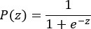   (9)

where p_(z) refers to the probability of class. Thus, the sigmoid activation allows us to calculate the probability of each class. The cross-entropy loss is used for training, and the predicted class will be the one with the highest probability.

Experimental analysis and results

The efficiency of the suggested model was tested using the Google Colab environment. It was implemented using the Python programming language. Due to its flexible architecture and broad library, it is one of the most commonly used languages for machine learning and scientific computing. For the evaluation of the suggested method, the confusion matrix was used. Even though accuracy can serve as a generalized performance indicator, its use may be misleading in case of the existence of imbalanced datasets. In addition to accuracy, evaluation measures such as recall, precision, and F1-score were used for more comprehensive model performance assessment. All the outputs and datasets are explained in Tables 1–9.

To ensure reproducibility, all experiments were conducted using a fixed experimental configuration. The proposed framework was implemented using Python-based deep learning libraries, with training performed on a CUDA-enabled GPU environment. EfficientNetB0 and ResNet50 were initialized using ImageNet pretrained weights and fine-tuned under the specified optimization settings. The dataset was divided before augmentation to prevent information leakage, and all generated samples were restricted to the training subset. Hyperparameters, augmentation parameters, optimization strategy, and model-selection criteria have been explicitly reported. The experimental settings and implementation parameters used for training and evaluating the CNN models are summarized.

The custom dataset used in this study consists of facial images collected from seven participants at Amman Arab University, Jordan. For each participant, the original face images were captured under unconstrained conditions involving variations in illumination, facial expressions, and partial occlusions. Due to the limited number of available samples, a neutrosophic-based data augmentation technique was applied to increase the dataset size. Table 1 shows the original and the neutrosophic dataset. Although the augmentation process contributes to improving model learning under limited-data conditions, the relatively small number of subjects remains a limitation that may affect the generalizability of the obtained results.

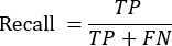
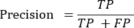
As mentioned previously, in binary classification problems, predictions can take four forms: true positive (TP), false positive (FP), true negative (TN), and false negative (FN). As shown in Table 3, the confusion matrix summarizes the possible outcomes of binary classification. Each component of the matrix has a specific interpretation, which is detailed in Table 4. These components form the basis for computing the evaluation metrics presented in Equations (10)–(13).

   (10)

   (11)

   (12)

   (13)

For the 32 images in the test set, the proposed framework correctly classified 31 images and incorrectly classified one image. Specifically, the confusion-matrix results consisted of 16 true positives (TP), 15 true negatives (TN), 1 false positive (FP), and 0 false negatives (FN). These values resulted in an accuracy of 96.9%, precision of 94.1%, recall of 100%, and F1-score of 96.9%. Reporting the integer confusion-matrix counts provides a direct verification of the performance measures, given the small size of the test set.

Furthermore, the area under the receiver operating characteristic curve (AUC) was used as an evaluation measure. The AUC takes values between 0 and 1; the closer the value is to 1, the better the separability of classes is. Otherwise, values close to 0 indicate that classification performance is rather weak. Table 5 represents a comparative evaluation of the proposed model against other algorithms using the neutrosophic datasets. The proposed ensemble model outperforms the other models in all categories, achieving 96.9% accuracy, 94.1% precision, 100% recall, and an F1-score of 96.9%.

Evaluation and selection of CNN architectures

To determine the most suitable CNN architectures for the proposed feature-fusion framework, eight CNN models were evaluated individually using both Original Data (OD) and Neutrosophic Data (ND), as presented in Table 2.  EfficientNetB0 and ResNet-50 achieved the strongest overall performance and were therefore selected for the proposed feature-fusion model. Both achieved 100% accuracy, precision, recall, and F1-score on OD, while on ND they achieved 93.75% accuracy, 88.89% precision, 100% recall, and 94.12% precision. The remaining architectures, VGG16, NASNetLarge, Xception, MobileNet, EfficientNetB0, ResNet-50, InceptionResNetV2, and MobileNetV2, were evaluated individually but were not selected for the final model. Figure 4 represents the dynamics of changes in the AUC score over time during training and validation for 50 epochs. Training AUC sharply rises at the beginning and reaches its maximum after 20 epochs. The same trend can be observed for the validation set, although its values increase at a lower pace, reaching their maximum at the 30th epoch. These graphs indicate that the algorithm has reached stable convergence.

Table 6 compares the computational characteristics of the proposed model with the baseline deep learning architectures using the neutrosophic datasets. The results indicate that the proposed approach requires a moderate training time of 352.76 s, which is lower than that of NASNetLarge (662.91 s) and InceptionResNetV2 (707.64 s), although it remains higher than the more lightweight architectures such as MobileNet and MobileNetV2. Its inference time of 199.77 ms per image places it within a competitive range, outperforming NASNetLarge, EfficientNetB0, ResNet50, and InceptionResNetV2, while remaining slightly slower than Xception, MobileNet, and MobileNetV2. The model size is 116.74 MB, reflecting a relatively substantial architecture compared with compact networks, but it is considerably smaller than NASNetLarge. In terms of parameterization, the proposed model contains 28.50 million total parameters, with approximately 0.86 million trainable parameters. Notably, its peak GPU memory consumption during training is 1481.53 MB, which is substantially lower than that of Xception and NASNetLarge. During inference, the proposed model records the lowest GPU memory requirement among all evaluated architectures, at only 208.76 MB. Overall, these results demonstrate that the proposed method provides a reasonable balance between computational cost, model complexity, inference efficiency, and memory utilization, particularly under inference conditions.

Table 7 summarizes the classification performance of the proposed model in comparison with the baseline deep learning architectures using the original dataset. The proposed model achieved perfect performance, obtaining 100% accuracy, precision, recall, and F1-score, with a processing time of 506.15 s. Comparable results were also observed for EfficientNetB0, ResNet50, and MobileNetV2, all of which achieved the same scores across the four evaluation metrics. Xception demonstrated strong performance, reaching 93.75% accuracy and an F1-score of 94.12%, while MobileNet produced an accuracy of 87.50% and an F1-score of 88.89%. NASNetLarge yielded comparatively lower performance, with 75% accuracy and an F1-score of 66.67%. In contrast, InceptionResNetV2 recorded the weakest results, achieving 50% accuracy and zero values for precision, recall, and F1-score. Although the proposed method required more processing time than several lightweight architectures, its perfect classification results indicate that it can achieve high predictive effectiveness on the original dataset while maintaining competitive performance relative to the evaluated baseline models. The experimental configuration and implementation parameters of the proposed framework are summarized in Table 8.

Table 9 presents the classification results obtained by the proposed model and three established face-recognition architectures, namely FaceNet, ArcFace, and CosFace, when evaluated on the neutrosophic dataset. The proposed model achieved the highest overall performance, with an accuracy of 96.9%, precision of 94.1%, recall of 100%, and an F1-score of 96.9%. CosFace provided the closest performance, attaining 93.8% accuracy and an F1-score of 94.1%, while also achieving complete recall. ArcFace showed a slightly lower accuracy of 90.6%, with precision, recall, and F1-score values of 84.2%, 100%, and 91.4%, respectively. FaceNet exhibited the lowest performance across the evaluated approaches, particularly in recall (25.0%) and F1-score (36.4%), despite achieving a precision of 66.7%. Overall, the results indicate that the proposed model offers a more balanced classification capability, combining high precision with complete recall and consequently achieving the strongest F1-score among the compared methods.

Figure 5 provides a comparative analysis of AUC scores among all tested models (A) EfficientNetB0 Model, (B) ResNet-50 Model, and (C) Xception Model. Figures 6–10  present the training and testing losses for different CNN architectures over 50 epochs for Xception, MobileNet, ResNet-50, NASNetLarge, and InceptionResNetV2 models. Typically, the training loss gradually drops throughout the whole training process. In contrast, testing loss tends to have peaks and, in certain cases, a steady growth trend, which indicates overfitting. Overfitting implies that the algorithm successfully learns features in the training data set but cannot generalize them to unseen samples. For instance, overfitting occurs in the Xception and ResNet-50 models, where training loss remains almost constant, but testing loss grows steadily. Therefore, there is a need to increase the level of regularization. Figure 11A–D demonstrates the overall performance of all models in terms of accuracy, precision, recall, and F1-score. Thus, the proposed hybrid model significantly outperforms other algorithms in all categories.

The experimental results indicate that combining complementary deep representations can improve verification performance on the evaluated dataset. However, the use of multiple CNN architectures also introduces additional computational requirements. In addition, because the size of the used dataset is quite small, the proposed framework should be viewed as a performance-oriented proof-of-concept rather than as a demonstrably computationally efficient solution.

DATA AVAILABILITY:

A collection of facial images used to train and evaluate the proposed facial recognition framework. The images represent different individuals and facial variations. The data are available on the following repository in the data explorer tab: https://www.kaggle.com/datasets/ibrahim2gad/facial-recognition

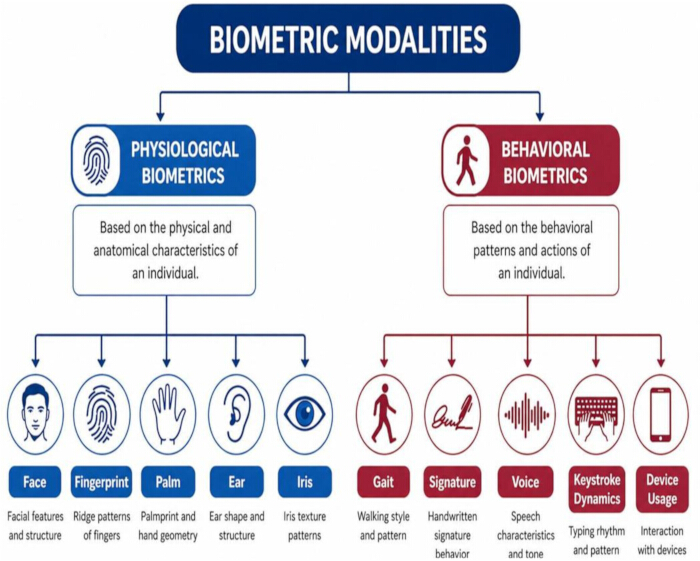
Figure 1: Classification of biometric modalities into physiological and behavioral categories. Biometric modalities are categorized as physiological biometrics, including face, fingerprint, palm, ear, and iris, and behavioral biometrics, including gait, signature, voice, keystroke dynamics, and device usage. Please click here to view a larger version of this figure.

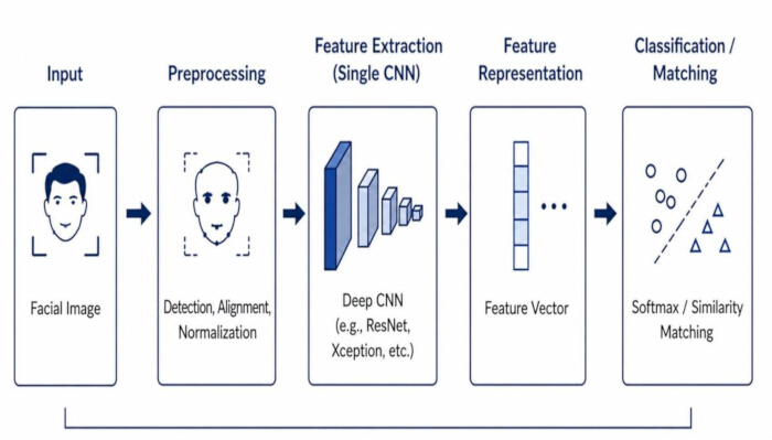
Figure 2: Standard facial recognition pipeline. The conventional single-model facial recognition workflow comprises facial image input, preprocessing through detection, alignment, and normalization, feature extraction using a CNN, feature representation as a feature vector, and final classification or similarity-based matching. Please click here to view a larger version of this figure.

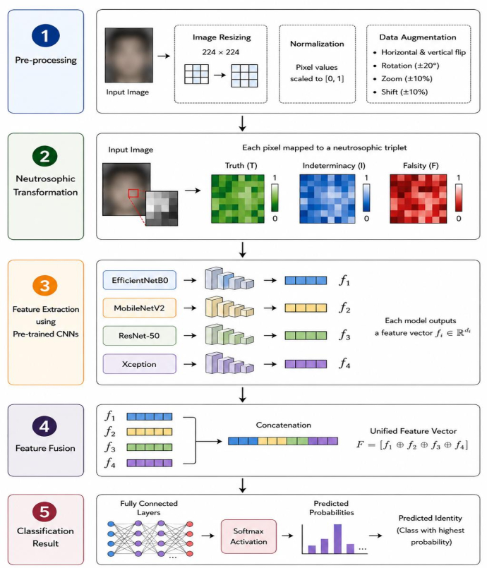
Figure 3: Overview of the proposed facial recognition framework. The proposed framework comprises sequential stages of image preprocessing, neutrosophic transformation into truth, indeterminacy, and falsity components, feature extraction using pretrained CNN models, concatenation of extracted features, and final classification using fully connected layers and Softmax activation. Please click here to view a larger version of this figure.

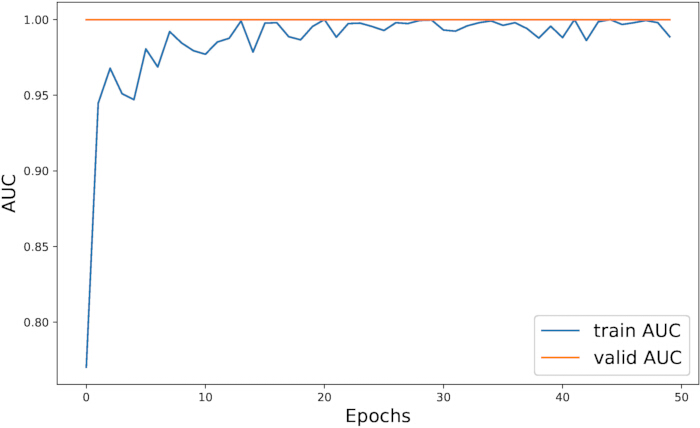
Figure 4: Training and validation AUC curves of the proposed model. Training and validation area under the curve (AUC) values are plotted across 50 epochs to illustrate the learning progression and convergence behavior of the proposed model. Please click here to view a larger version of this figure.

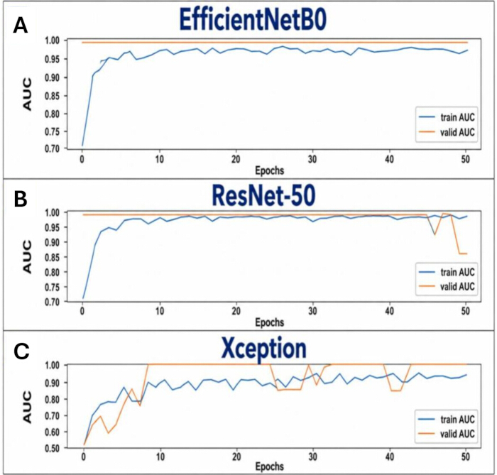
Figure 5: Comparative analysis of training and validation AUC curves across CNN models. Training and validation AUC values across 50 epochs are shown for (A) EfficientNetB0, (B) ResNet-50, and (C) Xception, illustrating differences in learning and validation performance among the evaluated models. Please click here to view a larger version of this figure.

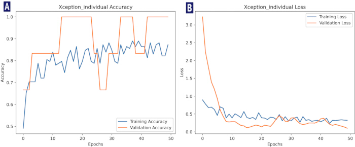
Figure 6: Training and validation performance of the Xception model. (A) Training and validation accuracy across 50 epochs. (B) Training and validation loss across 50 epochs. The curves illustrate the learning progression and generalization behavior of the Xception model. Please click here to view a larger version of this figure.

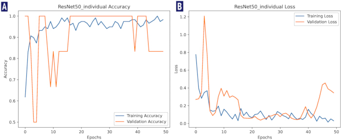
Figure 7: Training and validation performance of the ResNet-50 model. (A) Training and validation accuracy across 50 epochs. (B) Training and validation loss across 50 epochs. The curves illustrate the learning behavior and differences between training and validation performance of the ResNet-50 model. Please click here to view a larger version of this figure.

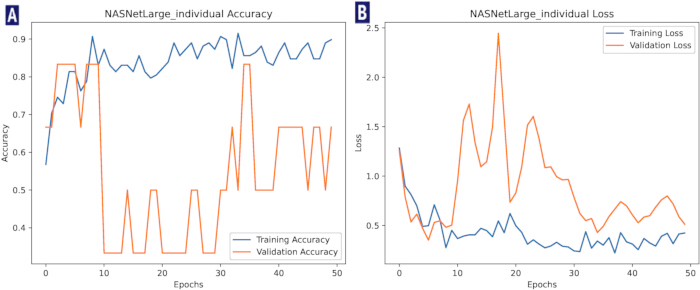
Figure 8: Training and validation performance of the NASNetLarge model. (A) Training and validation accuracy across 50 epochs. (B) Training and validation loss across 50 epochs. The curves demonstrate the training behavior and variation in validation performance of the NASNetLarge model. Please click here to view a larger version of this figure.

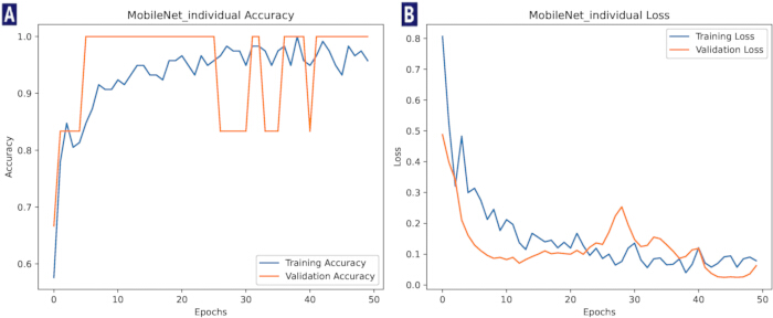
Figure 9: Training and validation performance of the MobileNet model. (A) Training and validation accuracy across 50 epochs. (B) Training and validation loss across 50 epochs. The curves illustrate the learning progression and validation performance of the MobileNet model. Please click here to view a larger version of this figure.

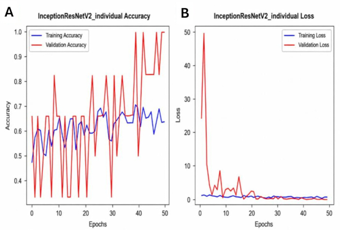
Figure 10: Training and validation performance of the InceptionResNetV2 model. (A) Training and validation accuracy across 50 epochs. (B) Training and validation loss across 50 epochs. The curves illustrate the convergence characteristics and differences between training and validation performance of the InceptionResNetV2 model. Please click here to view a larger version of this figure.

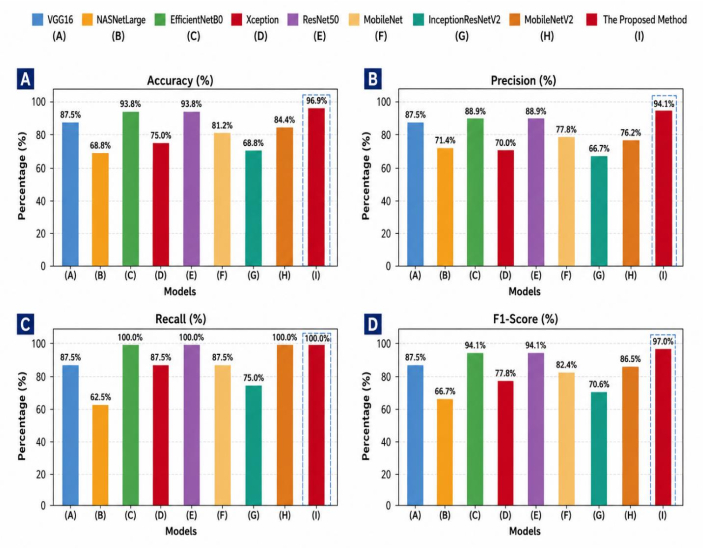
Figure 11: Performance comparison of the proposed method with baseline deep learning models. Comparative performance of the evaluated models is presented in terms of (A) accuracy, (B) precision, (C) recall, and (D) F1-score. Each panel compares VGG16, NASNetLarge, EfficientNetB0, Xception, ResNet50, MobileNet, InceptionResNetV2, MobileNetV2, and the proposed method. Please click here to view a larger version of this figure.

	Training set		Testing set		Total
	Yes	No	Yes	No
Original (OD)	34	25	8	8	75
Neutrosophic (ND)	68	50	16	16	150

Table 1: Distribution of data classes in the original and neutrosophic datasets. The distribution of data classes across the training and testing sets is presented for the original and neutrosophic datasets, showing the number of samples in each class.

CNN Architecture	Key Idea	Advantages	Limitations	Neutrosophic (ND)/ Original (OD) data
				Evaluated individually	Selected for Proposed model
EfficientNetB0	Compound scaling of depth, width, and resolution	High accuracy with fewer parameters	Requires careful tuning	Yes	Yes
ResNet-50	Residual learning with skip connections	Enables deep networks, stable training	Increased architectural complexity	Yes	Yes
MobileNetV2	Depthwise separable convolutions	Lightweight and computationally efficient	Slight trade-off in accuracy	Yes	NO
VGG16	Deep convolutional layers with small filters	Strong feature extraction and simple architecture	High number of parameters	Yes	NO
Xception	Depthwise separable convolutions (extreme Inception)	Efficient and powerful feature extraction	Higher computational cost than lightweight models	Yes	NO
MobileNet	Depthwise separable convolutions	Lightweight and computationally efficient	Slight trade-off in accuracy	Yes	NO
InceptionResNetV2	Inception modules with residual connections	Effective multi-scale feature extraction	High computational complexity	Yes	NO
NASNetLarge	Neural architecture search for optimized convolutional cells	High feature extraction capability	Large computational and memory requirements	Yes	NO

Table 2: CNN architectures used in the proposed framework. The CNN architectures evaluated in the proposed framework are summarized, including their key characteristics, advantages, limitations, evaluation status, and selection for the proposed model.

	Predicted Class
Actual Class	Positive	Negative
Positive	True Positive (TP)	False Negative (FN)
Negative	False Positive (FP)	True Negative (TN)

Table 3: Confusion matrix for binary classification. The confusion matrix structure for binary classification is presented, showing true positive, true negative, false positive, and false negative predictions.

True Positive (TP)	Correctly predicted positive instances
False Positive (FP)	Incorrectly predicted positive instances
True Negative (TN)	Correctly predicted negative instances
False Negative (FN)	Incorrectly predicted negative instances

Table 4: Interpretation of confusion matrix components. The components of the binary confusion matrix are defined, describing the interpretation of true positive, false positive, true negative, and false negative outcomes.

Model	Time	Accuracy (%)	Precision (%)	Recall (%)	F1-score (%)
VGG16	398.743	0.875	0.875	0.875	0.875
NASNetLarge	647.463	0.688	0.714	0.625	0.667
EfficientNetB0	427.686	0.938	0.889	1	0.941
Xception	426.405	0.75	0.7	0.875	0.778
ResNet-50	443.154	0.938	0.889	1	0.941
MobileNet	402.068	0.813	0.778	0.875	0.824
InceptionResNetV2	565.299	0.688	0.667	0.75	0.706
MobileNetV2	423.745	0.844	0.762	1	0.865
The proposed model	502.004	0.969	0.941	1	0.97

Table 5: Performance comparison of the proposed method with baseline models on the neutrosophic dataset. The performance of the proposed method is compared with baseline models using accuracy, precision, recall, F1-score, and computational time on the neutrosophic dataset.

	Training Time (s)	Inference Time (ms) per image	Model Size (MB)	Trainable Params	Total Params	GPU Mem Train Peak (MB)	GPU Mem Inference Peak (MB)
NASNetLarge	662.9129	248.5877	339.417	1040769	85965651	3909.9656	541.4707
EfficientNetB0	284.3383	219.3711	20.0655	330753	4382884	748.6084	550.8516
Xception	282.7168	194.7422	86.1482	528897	21394473	5451.2883	652.5537
ResNet50	298.5304	211.9212	96.6928	528897	24120705	1557.0549	784.9333
MobileNet	242.1108	179.548	15.6827	264705	3495617	1553.9807	772.9109
InceptionResNetV2	707.6381	250.3113	214.4063	396801	54736609	1734.147	1042.1941
MobileNetV2	253.5079	178.9581	12.9866	330753	2591297	1482.0718	1049.4602
The proposed model	352.755	199.7726	116.7427	859649	28503588	1481.5283	208.7615

Table 6: Computational performance and resource utilization of the proposed and baseline models. The computational efficiency and resource requirements of the proposed model and baseline models are compared using training and inference time, model size, parameter count, and GPU memory utilization.

Model	Time	Accuracy (%)	Precision (%)	Recall (%)	F1-score (%)
NASNetLarge	683.1349	0.75	1	0.5	0.6667
EfficientNetB0	444.8527	1	1	1	1
Xception	446.4684	0.9375	0.8889	1	0.9412
ResNet50	451.4806	1	1	1	1
MobileNet	404.8636	0.875	0.8	1	0.8889
InceptionResNetV2	576.889	0.5	0	0	0
MobileNetV2	418.7009	1	1	1	1
The proposed model	506.1484	1	1	1	1

Table 7: Performance comparison of the proposed method with baseline models on the original dataset. The classification performance of the proposed method and baseline deep learning models on the original dataset is compared using the reported performance metrics.

Parameter	Value
Dataset	Custom facial dataset
Input size	180 × 180
CNN architectures	VGG16, EfficientNetB0, ResNet-50, MobileNet, MobileNetV2, Xception, InceptionResNetV2, NASNetLarge.
Pretrained weights	ImageNet
Optimizer	Adam
Learning rate	0.001
Batch size	32
Epochs	50
Random seed	1337
GPU	Tesla T4, 15360 MiB
CUDA	12.5.1
Python	3.13.15
PyTorch	2.1.x
TensorFlow	2.20.x
Keras	2.14.x
Decision threshold	0.5
Augmentation	Random horizontal and vertical flips, rotation (up to 20◦), zooming (up to 10%), and shifting (up to 10%).

Table 8: Experimental settings and implementation parameters of the proposed framework.
The experimental configuration and implementation parameters of the proposed framework are summarized, including dataset settings, model architectures, optimization parameters, training settings, and computational environment.

Model	Accuracy (%)	Precision (%)	Recall (%)	F1-score (%)
FaceNet	0.563	0.667	0.250	0.364
ArcFace	0.906	0.842	1.000	0.914
CosFace	0.938	0.889	1.000	0.941
The proposed model	0.969	0.941	1	0.969

Table 9: Performance comparison of the proposed model with FaceNet, ArcFace, and CosFace on the neutrosophic dataset. The performance of the proposed model is compared with FaceNet, ArcFace, and CosFace on the neutrosophic dataset using the reported classification performance metrics.

讨论

The experimental results demonstrate that the proposed hybrid deep learning framework significantly improves facial recognition performance under uncontrolled environmental conditions. Unlike traditional single-model CNN approaches, the proposed method benefits from integrating complementary deep features extracted from multiple pre-trained architectures, including EfficientNetB0 and ResNet-50. Each model contributes unique discriminative characteristics, enabling the framework to better handle variations in facial expressions, illumination, occlusion, and image noise commonly encountered in real-world scenarios.

The feature-level fusion strategy played a critical role in enhancing recognition accuracy by combining the strengths of the best-performing CNN models while reducing the limitations associated with individual architectures. Furthermore, the smoothing and flattening operations applied to the fused feature vectors improved feature consistency and reduced redundancy, which positively affected the classification performance and computational efficiency of the system. The proposed framework achieved an accuracy of 96.9%, precision of 94.1%, recall of 100%, and an F1-score of 96.9%, outperforming all standalone CNN models evaluated in the study. The perfect recall value indicates the system’s strong capability to correctly identify positive facial instances without missing relevant samples, which is particularly important in security and surveillance applications. Additionally, the high F1-score demonstrates a balanced trade-off between precision and recall, confirming the robustness and reliability of the proposed approach.

Despite its promising performance, the proposed approach has several limitations. First, the use of multiple deep models increases computational complexity during both training and inference, which may limit real-time deployment on resource-constrained devices. Second, the evaluation is conducted on a dataset, which may not fully capture the diversity of real-world conditions, potentially affecting generalizability. Third, the feature fusion process, although effective, may introduce redundancy and increased dimensionality, which could impact scalability if not carefully optimized. Other approaches could be explored to validate and extend the proposed hypothesis. For instance, attention-based mechanisms, such as Vision Transformers (ViTs), could be used to dynamically weight important facial regions instead of relying on static CNN feature extraction^{32,33,34,35,36}.

The proposed hybrid framework has significant implications across multiple application domains. In security and surveillance systems, the high recall (100%) ensures minimal false negatives, which is critical for threat detection and access control. In smart retail and authentication systems, improved recognition accuracy enhances user experience and system reliability. Future research can focus on reducing computational overhead through model compression techniques such as pruning, quantization, or knowledge distillation. Additionally, exploring adaptive or learnable fusion strategies could further improve feature integration by dynamically selecting the most relevant features³⁷. Expanding the evaluation to larger and more diverse datasets would enhance the generalizability of the findings. Finally, integrating emerging architectures such as transformers or hybrid CNN-transformer models may further boost performance and open new avenues for robust facial recognition systems.

Although the proposed framework demonstrates promising performance on the collected dataset, the limited number of subjects and testing samples represents an important limitation. Therefore, the obtained results should be interpreted as a proof-of-concept evaluation rather than evidence of immediate applicability in large-scale real-world systems. Applications such as banking, military identification, and surveillance require extensive validation using large and diverse datasets containing variations in demographic characteristics, illumination, pose, occlusion, image quality, and acquisition conditions. Future work will focus on validating the proposed framework using larger publicly available facial recognition benchmarks and more challenging evaluation protocols. These experiments will include controlled analyses of individual factors, including illumination variation, occlusion levels, pose changes, facial expression diversity, image degradation, and noise robustness, to provide a more comprehensive assessment of generalization capability. In addition, the current evaluation does not establish performance across independent external datasets or large-scale contemporary face-recognition benchmarks. The small number of participants also prevents a reliable assessment of demographic variability and population-level generalization. Consequently, the present results should be interpreted as a proof-of-concept evaluation of the proposed methodology.

This work proposes a novel framework for facial recognition based on the fusion of different pre-trained deep CNNs (EfficientNetB0 and ResNet-50)^{13,14,15,16,17}. Using the method of feature fusion combined with neutrosophic representation allows addressing the issues of uncertainty, variation in facial conditions, and the small volume of data used. According to experimental results, the accuracy of the proposed algorithm was 96.9%. Extensive research, including testing the model performance using metrics like accuracy, precision, recall, F1-score, and AUC values, shows that the use of multiple complementary feature representations is highly effective³⁸, leading to better generalization and classification in real-world situations.

材料

本文使用的材料清单

姓名	公司	目录编号	评论
GPU Acceleration Platform: CUDA Toolkit	NVIDIA Corporation	12.1	GPU acceleration for deep learning operations
Cloud Computing Environment: Google Colab	Google Research	2025 environment	GPU-enabled model development and experimentation
Notebook Environment: Jupyter Notebook	Project Jupyter	7.x	Interactive experimentation and analysis
High-Level Neural Network API: Keras	François Chollet / Google	2.14.x	Rapid construction and training of neural networks
Data Visualization: Matplotlib	Matplotlib Development Team	3.8.x	Plot generation and result visualization
Numerical Computing Library: NumPy	NumPy Developers	1.26.x	Matrix operations and numerical processing
Image Processing Library: OpenCV	OpenCV Team	4.8.x	Image preprocessing, transformation, and computer vision operations
Data Processing Library: Pandas	The Pandas Development Team	2.1.x	Dataset loading, cleaning, and feature manipulation
Programming Language: Python	Python Software Foundation	3.10.x	Main programming language for data processing, model development, and evaluation
Deep Learning Framework: PyTorch	Meta AI / PyTorch Team	2.1.x	Training and inference of deep learning architectures
Machine Learning Library: Scikit-learn	Scikit-learn Developers	1.3.x	Classical ML algorithms, evaluation metrics, preprocessing
Scientific Computing Library: SciPy	SciPy Community	1.11.x	Optimization and scientific computations
Deep Learning Framework: TensorFlow	Google Brain / Google LLC	2.14.x	Deep learning model implementation and experimentation
Operating System: Ubuntu Linux	Canonical Ltd.	22.04 LTS	Experimental computing environment and GPU-based model training