Rethinking Urgency Cues: Scarcity Messaging, Credibility, and Purchase Intention in a Survey of Social Media Fruit Advertising

摘要

Scarcity Message Intensity was positively associated with perceived credibility and fear of missing out (FOMO), with significant indirect associations with purchase intention. Consumer skepticism strengthens the scarcity–FOMO relationship, while household income shows no significant moderating effect.

摘要

Scarcity appeals are widely used in social media advertising, yet their influence on purchase intention may involve both cognitive and affective mechanisms. This study examines the relationships between scarcity message intensity and purchase intention through perceived credibility and fear of missing out (FOMO), with consumer skepticism and household income level as moderators. Drawing on the Elaboration Likelihood Model, Signaling Theory, and the Persuasion Knowledge Model, survey data from 272 Chinese social-commerce users were analyzed using partial least squares structural equation modeling (PLS-SEM). Scarcity message intensity was positively associated with perceived credibility, contrary to the negative relationship proposed in Hypothesis 1, and was also positively associated with FOMO. Both perceived credibility and FOMO were positively associated with purchase intention. Although the direct relationship between scarcity message intensity and purchase intention was non-significant, both indirect pathways were positive and statistically significant, with the indirect effect through perceived credibility larger than that through FOMO. Consumer skepticism significantly moderated the scarcity–FOMO relationship, but in the direction opposite to that hypothesized; therefore, H6 was not supported. Household income did not significantly moderate the perceived credibility–purchase intention relationship, and H7 was not supported.

引言

In contemporary digital commerce, scarcity tactics, particularly algorithm- and digital-technology-driven urgency cues such as countdown timers and low-stock alerts, have become ubiquitous features of e-commerce platforms¹. Scarcity theory proposes that perceived scarcity can increase purchase intention through heightened urgency; however, the proliferation of such cues in digital environments has increasingly invited scrutiny. For inherently perishable products such as fresh agricultural goods, excessive urgency messaging may induce consumer fatigue and skepticism². Scarcity marketing can therefore trigger impulsive emotional reactions³ while also prompting deliberate cognitive reflection⁴, creating a psychological effect inadequately explained by traditional unitary models⁵.

The global fresh e-commerce market has grown rapidly and is now worth more than US$1.2 trillion⁶, with social commerce platforms using product videos and real-time stock alerts to encourage purchases⁷. Despite this growth, three theoretical gaps remain. First, prior research has predominantly examined the affective pathway through which scarcity enhances purchase intention via fear of missing out (FOMO), while giving less attention to the cognitive possibility that intense scarcity messaging may enhance perceived advertising credibility by signaling product quality and rapid turnover⁵. Second, scarcity is often treated as a unidimensional stimulus without distinguishing the concurrent emotional (FOMO) and cognitive (credibility) mechanisms or recognizing that both pathways may operate concurrently in shaping purchase intention despite a non-significant direct effect⁸. Third, the boundary conditions determining pathway dominance remain insufficiently specified because individual differences such as chronic skepticism and socioeconomic status, including household income, are typically examined separately⁹.

To address these gaps, this study proposes and empirically tests a dual-pathway model linking scarcity message intensity to purchase intention. Scarcity intensity may simultaneously activate an affective pathway, in which urgency triggers FOMO and impulsive decision-making, and a cognitive pathway, in which consumers evaluate the credibility of scarcity claims. This simultaneous treatment distinguishes the present framework from approaches that examine scarcity primarily as a direct antecedent of purchase intention or focus on a single psychological mechanism. The model further considers consumer skepticism and household income as boundary conditions that may alter the relative importance of these pathways. The novelty of this study therefore lies in integrating cognitive and affective responses within a single framework while examining whether individual and socioeconomic differences shape their operation. By applying this framework to social media advertising for perishable fruit products, the study extends unidimensional explanations of scarcity marketing and examines when scarcity messages may be effective or counterproductive in digitally mediated commerce.

The theoretical framework integrates scarcity theory, the Elaboration Likelihood Model (ELM)¹⁰, Signaling Theory¹¹, the Persuasion Knowledge Model (PKM)¹², and Reactance Theory¹³. Scarcity theory holds that limited availability can heighten perceived value and stimulate purchasing, while FOMO provides an affective mechanism through which scarcity may encourage impulsive buying⁹. However, repeated artificial urgency cues in algorithm-saturated marketplaces can foster skepticism, complicating a simple positive relationship¹⁴. Socioeconomic differences may further shape responses; consumers with higher household incomes may interpret aggressive scarcity appeals as signals of lower quality, whereas budget-constrained consumers may be more vulnerable to FOMO¹⁵.

ELM provides the overarching dual-route framework¹⁰. Scarcity message intensity can function through a peripheral route, in which urgency triggers FOMO through loss aversion and heuristic processing, and a central route, in which consumers evaluate the credibility and authenticity of the message¹⁰. These processes can operate concurrently rather than representing mutually exclusive responses to scarcity cues. Signaling Theory further suggests that, particularly for perishable goods, intense scarcity messages may function as credible signals of rapid inventory turnover and freshness rather than manipulation¹¹. Thus, perceived credibility can become a positive cognitive appraisal rather than functioning solely as a defensive filter. Although the cognitive and affective pathways may both positively influence purchase intention, they can differ in their relative dominance within the decision-making process. Their simultaneous operation provides a theoretical basis for examining whether scarcity influences purchase intention through concurrent indirect pathways¹⁶.

PKM and Reactance Theory inform the moderating role of skepticism. Highly skeptical consumers are more likely to scrutinize persuasive intent and may resist scarcity appeals^12,13. Income provides a socioeconomic boundary condition; greater financial latitude may facilitate deliberative processing and greater reliance on credibility, whereas lower-income consumers may be more sensitive to temporal pressure and FOMO¹⁵. Accordingly, ELM provides the dual-route structure¹⁰, Signaling Theory explains the potential positive credibility pathway¹¹, and PKM and Reactance Theory explain relevant boundary conditions^12,13.

Scarcity message intensity refers to the degree to which marketing communications emphasize restrictive or urgency-related cues, such as limited stock, expiring offers, or high demand, to create perceptions of limited product availability ¹⁴. In digital social commerce, these cues may include limited-stock notifications, time-limited offers, and indicators of elevated consumer demand. When such cues restrict or appear to restrict consumers’ freedom of choice, they may generate psychological pressure and reactance ¹⁷. In the present study, these related scarcity and urgency cues are conceptualized collectively as scarcity message intensity (SMI) to capture the overall strength of perceived scarcity communicated by the advertisement.

Prior findings concerning scarcity effectiveness are mixed. Scarcity theory and loss-aversion perspectives suggest that intense scarcity can increase purchase intention by eliciting impulsive emotional responses, particularly FOMO⁹, with meta-analytic evidence indicating increased conversion under scarcity conditions¹⁸. Conversely, PKM and Reactance Theory suggest that overused or apparently algorithm-driven scarcity cues can generate skepticism and resistance, with many online consumers questioning their authenticity^12,13,14. The affective pathway is expected to increase purchase intention, whereas the credibility pathway presents a more complex theoretical prediction. From PKM and Reactance Theory, greater scarcity intensity may increase suspicion of manipulative intent and reduce perceived credibility ^12,13.

At the same time, scarcity-induced urgency and FOMO may encourage purchase-related responses⁹. Thus, the affective pathway supports a predicted positive relationship with purchase intention, whereas the cognitive credibility pathway may offset this effect.

H1: Scarcity message intensity has a negative association with perceived credibility.

H2: Scarcity message intensity has a positive association with purchase intention.

H3: Scarcity message intensity has a positive association with FOMO.

Perceived credibility reflects consumers’ evaluation of the truthfulness, authenticity, and reliability of advertising claims⁵. In social media scarcity marketing, it concerns whether limited-inventory warnings are interpreted as genuine supply constraints or potentially manipulative scarcity claims ^14,17. Compromised credibility may reduce purchase likelihood, particularly for perishable products, for which authenticity can influence product evaluations¹⁵. Scarcity and urgency cues can enhance product desirability and purchase-related responses⁴, whereas suspected artificial scarcity may activate persuasion knowledge and resistance ^12,14,17. Social commerce users may consequently approach AI-generated or algorithmically delivered urgency cues with skepticism^1,7. When scarcity messages are perceived as genuine, greater credibility can strengthen purchase intention. Accordingly:

H4: Perceived credibility has a positive association with purchase intention.

FOMO is a psychologically distressing state involving apprehension that others may experience rewarding opportunities from which an individual is absent¹⁹. In consumer contexts, it manifests as anxiety about missing time-limited opportunities and can override rational cost-benefit evaluations²⁰. Scarcity stimuli can produce physiological arousal that accelerates decision-making toward immediate acquisition^4,21. Although responses to FOMO may vary across consumers and contexts, prior research generally supports a positive association between FOMO and purchase-related intentions^9,21. Despite this potential curvilinear pattern, the predominant effect across the relevant intensity range is expected to remain positive.

H5: FOMO has a positive association with purchase intention.

Consumer skepticism is a stable tendency to question and critically evaluate marketing claims²² and can function as a psychological defense against perceived manipulation²³. Highly skeptical consumers may interpret scarcity warnings as algorithmic or deceptive rather than genuine constraints, encouraging systematic evaluation of message authenticity. Skepticism is therefore proposed as an attenuating moderator of the affective pathway. For highly skeptical consumers, cognitive evaluation may interrupt the automatic translation of urgency into FOMO because they recognize the persuasive intent underlying the scarcity appeal^24. Consequently, the positive relationship between scarcity message intensity and FOMO is predicted to weaken as skepticism increases.

H6: Consumer skepticism negatively moderates the relationship between scarcity message intensity and FOMO, such that the positive effect of intensity on FOMO is weaker for consumers with higher skepticism.

Household income is proposed as a socioeconomic moderator of the cognitive pathway. In the present study, income is treated as an observed socioeconomic characteristic that may differentiate consumers’ responses to scarcity-based advertising. Consumers with greater financial resources may experience fewer budget constraints and greater flexibility in their purchasing decisions. Accordingly, household income is examined as a potential moderator of the relationship between perceived credibility and purchase intention.

H7: Household income positively moderates the relationship between perceived credibility and purchase intention, such that the positive relationship is stronger at higher levels of household income.

Accordingly, the objective of the study was to test the direct, indirect, and moderating relationships represented by H1–H7 within the proposed dual-pathway framework.  Figure 1 illustrates the proposed model examining scarcity messaging in social media fruit advertising, emphasizing the dual psychological pathways of FOMO and perceived credibility, with consumer skepticism and household income level as moderators.

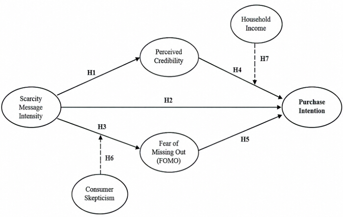
Figure 1: Proposed research model. The model illustrates the hypothesized direct relationships among Scarcity Message Intensity, Perceived Credibility, fear of missing out (FOMO), and Purchase Intention (H1–H5), as well as the moderating effects of Consumer Skepticism on the relationship between Scarcity Message Intensity and FOMO (H6) and Household Income on the relationship between Perceived Credibility and Purchase Intention (H7). Solid arrows indicate direct hypothesized relationships, and dashed arrows indicate hypothesized moderating effects. Please click here to view a larger version of this figure.

方案

Ethical approval for this study was provided by the Ethics Committee of Guangxi Tianhong Certified Public Accountants Co., Ltd. (Ethics Review No. 20240608). The study included only adult participants aged 18 years or older. Electronic informed consent was obtained from all participants through the online questionnaire prior to participation. Participants were informed about the study purpose, procedures, potential benefits and risks, and the voluntary nature of their participation. Participant privacy and confidentiality were protected, and all study data were de-identified.

Research design

This study used a quantitative cross-sectional survey design to examine the affective and cognitive pathways linking scarcity message intensity with purchase intentions in social media fruit advertising, as well as the moderating effects of consumer skepticism and income level. A three-phase analytical approach was used: (1) preliminary data screening and reliability analysis using IBM SPSS Statistics (version 26); (2) measurement model assessment using SmartPLS 4.0; and (3) structural model, mediation, and moderation analyses using SmartPLS 4.0.

Participants and Sampling Procedure

Data were collected from January 15, 2026, to February 28, 2026, in the People’s Republic of China. China was selected as the study context because of its highly developed social-commerce environment. Platforms such as Douyin, Xiaohongshu, and Taobao Live routinely incorporate urgency cues, including limited-stock notifications, flash-sale promotions, countdown displays, and real-time demand indicators, into online purchasing environments, providing an appropriate context for examining the dual-pathway effects of scarcity message intensity. A purposive sampling technique was used to recruit respondents with relevant experience in online fruit purchasing and exposure to scarcity-related advertising.

Questionnaire invitation links were disseminated through online consumer communities and social-commerce discussion groups associated with Douyin, Xiaohongshu, and Taobao Live. The invitation briefly described the study and directed interested respondents to the self-administered online questionnaire.

Eligibility for the focal consumer-experience criteria was assessed through screening questions presented before the main questionnaire. Respondents were asked whether they had purchased fresh fruit online within the preceding three months and whether they had encountered at least one scarcity-themed fruit advertisement, such as “limited stock” or “flash sale ending soon,” within the previous month. Only respondents satisfying both consumer-experience criteria were retained in the eligible response pool.

Responses were subsequently screened for completeness, consumer-experience eligibility, and age eligibility before analysis. Incomplete responses, cases that did not satisfy the consumer-experience criteria, and responses from individuals younger than 18 years were excluded. The final analytical sample comprised 272 adult participants aged 18 years or older, and this adult-only sample was used for all subsequent analyses. The de-identified item-level dataset for the final analytical sample is provided in Supplementary Data File 1.

Statistical power was assessed using the F-test framework for linear multiple regression (fixed model, R² deviation from zero). The most complex endogenous equation, Purchase Intention, contained five predictors: Scarcity Message Intensity, Perceived Credibility, FOMO, Household Income Category, and the Perceived Credibility × Household Income interaction term. Assuming a medium effect size (f² = 0.15), α = 0.05, five predictors, and 0.80 statistical power, 92 participants were required. The final analytical sample of 272 participants therefore exceeded the minimum sample-size requirement.

Methodological Considerations and Contextual Boundaries

The Chinese social-commerce context provides a valuable setting for examining real-world scarcity cues, but several boundaries should be acknowledged. Cultural context and familiarity with digitally curated content may influence responses to scarcity, social proof, FOMO, and skepticism, potentially limiting generalizability to other settings. In addition, differences in platform design across Douyin, Xiaohongshu, and Taobao Live may affect how scarcity cues are processed. Although multi-platform recruitment reduces reliance on a single platform, the study does not permit platform-specific comparisons.

The purposive sampling criteria further limit generalizability to consumers with recent online fruit-purchasing experience. The sample was also concentrated among younger adults and relatively higher-income consumers, who may differ from older, lower-income, or less digitally engaged populations in their responses to online urgency cues. Accordingly, the findings should be interpreted primarily within the context of Chinese social commerce and should not be directly generalized to offline retail or other cultural and demographic settings. Future research should examine these relationships across countries, demographic groups, platforms, and retail environments.

Table 1 presents the demographic and purchasing profile of the final adult sample (N = 272). Participants were predominantly aged 26–35 years (40.1%), followed by 36–45 years (26.1%), 18–25 years (23.9%), and 46 years or older (9.9%). Females represented 56.6% of the sample. Most participants reported monthly household incomes above ¥8,000 (67.3%), while monthly fruit expenditure was most commonly ¥101–300 (37.5%). Overall, the sample primarily comprised

young to middle-aged adults and relatively higher-income consumers with varied income and fruit-purchasing profiles.

Characteristic	Category	n	Percentage (%)
Age (years)	18–25	65	23.9
	26–35	109	40.1
	36–45	71	26.1
	≥46	27	9.90
Gender	Male	118	43.4
	Female	154	56.6
Monthly household income (RMB)	≤3,000	31	11.4
	3,001–8,000	58	21.3
	8,001–15,000	106	39.0
	>15,000	77	28.3
Monthly fruit expenditure (RMB)	≤100	79	29.0
	101–300	102	37.5
	301–500	54	19.9
	501–800	27	9.9
	>800	10	3.7

Table 1: Demographic Characteristics and Purchasing Profile of Participants (N = 272).

Demographic characteristics and purchasing profile of the participants, including age, gender, monthly household income, and monthly fruit expenditure. Household Income was coded into four categories: 1 = <3,000 RMB; 2 = 3,001–8,000 RMB; 3 = 8,001–15,000 RMB; and 4 = >15,000 RMB.

Measures

All continuous constructs were measured using multi-item scales rated on a five-point Likert scale ranging from 1 (Strongly Disagree) to 5 (Strongly Agree). Household income was measured separately using four categorical monthly income brackets. The complete bilingual questionnaire, including the English and Simplified Chinese items, response scales, and coding instructions, is provided in Supplementary Data File 2.

The measurement items for each construct are detailed below, with representative sample items provided to illustrate the content domain.

Scarcity Message Intensity (3 items) was adapted from Gierl and Huettl²⁵, capturing the perceived strength of scarcity and urgency cues. Representative items included: “The advertisement emphasized that this fruit was available in a very limited quantity,” “The promotional message strongly highlighted the short time available to purchase,” and “The advertisement conveyed that this fruit was in high demand with limited supply.”

Perceived Credibility (5 items) was measured using scales from MacKenzie and Lutz²⁶ and Pornpitakpan²⁷, assessing consumers’ trustworthiness evaluations of the scarcity claims. Representative items included: “I believe the claims made in the fruit advertisement are authentic,” “The merchant providing the scarcity advertisement appears trustworthy,” and “The promotional countdown and stock indicators seem genuine.”

Fear of Missing Out (FOMO; 6 items) was adapted from Przybylski et al.¹⁹, capturing FOMO associated with potentially missed opportunities. Representative items included: “I worried that others would purchase the discounted fruit before I did,” “I felt a strong fear of missing out on this limited fruit deal,” and “Missing this promotion would feel like a financial loss.”

Purchase Intention (6 items) was assessed using scales from Dodds et al.²⁸ and Spears and Singh²⁹, measuring the likelihood of product acquisition. Representative items included: “I plan to buy the advertised fruit in the near future,” “I am willing to purchase this fruit during the scarcity campaign,” and “It is very likely that I will order this fresh fruit online.”

Consumer Skepticism (6 items) was adapted from Obermiller and Spangenberg³⁰. Representative items included “I tend to be skeptical of scarcity claims in social commerce fruit ads,” “Most scarcity-themed fruit advertisements are exaggerated,” and “I doubt that flash sales reflect true inventory shortages.”

Content validity was assessed by three marketing academics and two senior e-commerce practitioners. Each expert rated the relevance of individual items on a four-point scale (1 = not relevant, 2 = somewhat relevant, 3 = quite relevant, and 4 = highly relevant). The item-level content validity index (I-CVI) was calculated as the proportion of experts assigning a rating of 3 or 4 to each item. All items met the acceptable criterion of I-CVI ≥ 0.78, with only minor wording refinements required. A pilot test was subsequently conducted with 50 respondents who met the same eligibility criteria as the main study to assess questionnaire clarity, comprehensibility, and completion time (approximately 8 min). Pilot participants were excluded from the final analytical sample. Internal consistency was assessed using the final adult sample (N = 272), and all constructs demonstrated satisfactory reliability. No substantive changes to the final instrument were required.

Data Analysis Strategy

Data analysis was conducted in three sequential phases using IBM SPSS Statistics (version 26) for preliminary analyses and SmartPLS 4.0 for PLS-SEM. Phase 1 involved data cleaning, descriptive analysis, and reliability assessment. Responses were screened for participant eligibility, completeness, missing values, and values outside the permitted response ranges. Cases not meeting the eligibility requirements, including respondents younger than 18 years, were excluded. Missing data were identified by checking each analytical variable for blank or unavailable responses; cases lacking data required for the analysis were excluded rather than imputed. Following cleaning, the final adult analytical sample comprised N = 272, with no missing values.

Internal consistency was assessed using Cronbach’s α. Sampling adequacy was evaluated using the Kaiser–Meyer–Olkin (KMO) measure and Bartlett’s test of sphericity. Exploratory factor analysis (EFA) was conducted using principal axis factoring with Varimax rotation. Factors were retained based on eigenvalues > 1.0 together with inspection of the scree plot. Items were expected to have a primary factor loading of ≥ 0.50 and no substantial cross-loading (≥ 0.30) on another factor. Items failing these criteria were considered for removal based on both statistical performance and conceptual relevance.

Phase 2 involved measurement-model assessment using SmartPLS 4.0. Convergent validity was evaluated using indicator loadings (preferably ≥ 0.70; loadings ≥ 0.60 considered acceptable when construct reliability and validity remained satisfactory), composite reliability (CR ≥ 0.70), and average variance extracted (AVE ≥ 0.50). Discriminant validity was assessed using the Fornell–Larcker criterion and the heterotrait–monotrait ratio (HTMT < 0.85). Model fit was assessed using the normed fit index (NFI) obtained from SmartPLS 4.0, with a value > 0.90 used as the stated acceptance criterion. Phase 3 involved structural-model assessment and hypothesis testing. Path coefficients, standard errors, t statistics, p values, and 95% bootstrap confidence intervals were estimated from 5,000 bootstrap resamples using two-tailed significance testing at α = 0.05. An effect was considered statistically significant when p < 0.05 and its 95% bootstrap confidence interval did not include zero.

Moderation was evaluated by constructing the specified interaction terms in SmartPLS 4.0. For H6, the continuous variables Scarcity Message Intensity and Consumer Skepticism were mean-centered to construct the Scarcity Message Intensity × Consumer Skepticism interaction term. Conditional effects were interpreted at the mean and one standard deviation below and above the mean (−1 SD, mean, +1 SD). H7 was represented by the Perceived Credibility × Household Income interaction term using the four-category Household Income variable reported in Table 1.

Mediation was evaluated using bootstrapped direct and specific indirect effects. An indirect effect was considered statistically significant when its 95% bootstrap confidence interval excluded zero. Mediation type was determined by jointly examining the significance and direction of the direct and indirect effects. A significant indirect effect accompanied by a non-significant direct effect was classified as indirect-only mediation. The PLS algorithm used the path-weighting scheme with a maximum of 300 iterations.

Common Method Bias

Because all data were self-reported, common method bias was addressed through procedural and statistical measures. Procedurally, responses were collected anonymously, and predictor, mediator, and criterion variables were presented in separate questionnaire sections to reduce response-pattern and proximity effects. Statistically, Harman’s single-factor test was conducted using the continuous construct items. The first factor accounted for 31.70% of the total variance, below the 50% criterion. Thus, no single factor accounted for the majority of the variance, suggesting that common method bias was unlikely to dominate the observed relationships.

结果

Descriptive Statistics

Table 2 presents the descriptive statistics for the study variables. Perceived Credibility had the highest mean score (M = 3.90, SD = 0.91), followed by Scarcity Message Intensity (M = 3.72, SD = 1.07), FOMO (M = 3.71, SD = 0.96), Purchase Intention (M = 3.61, SD = 1.06), and Consumer Skepticism (M = 3.57, SD = 1.06). Household Income had a mean coded category of 2.84 (SD = 0.96). Skewness values ranged from −1.25 to −0.45 and kurtosis values ranged from −1.30 to 0.24, indicating no severe univariate distributional departures. The observed ranges also demonstrated adequate variability across the study variables.

Construct/Variable	Mean	SD	Skewness	Kurtosis	Min	Max
Scarcity Message Intensity	3.72	1.07	−0.98	−0.29	1.00	5.00
Perceived Credibility	3.90	0.91	−1.25	0.24	1.60	5.00
FOMO	3.71	0.96	−1.00	−0.52	1.50	5.00
Purchase Intention	3.61	1.06	−0.77	−0.97	1.33	5.00
Consumer Skepticism	3.57	1.06	−0.55	−1.30	1.33	5.00
Household Income	2.84	0.96	−0.45	−0.75	1.00	4.00

Table 2: Descriptive Statistics of Study Variables.

Mean, standard deviation (SD), skewness, kurtosis, minimum, and maximum values for the study variables in the final analytical sample (N = 272). Scarcity Message Intensity, Perceived Credibility, fear of missing out (FOMO), Purchase Intention, and Consumer Skepticism were measured on five-point scales. Household Income was coded into four categories from 1 to 4.

Table 3 shows the Pearson correlations among the study variables. Scarcity Message Intensity was positively correlated with Perceived Credibility (r = 0.429), Purchase Intention (r = 0.404), FOMO (r = 0.429), and Consumer Skepticism (r = 0.320), but showed essentially no correlation with Household Income (r = −0.004). Purchase Intention was positively correlated with Perceived Credibility (r = 0.482), FOMO (r = 0.409), and Consumer Skepticism (r = 0.478), whereas its correlation with Household Income was weak (r = 0.046). Overall, Household Income showed only negligible to weak correlations with the study constructs (r = −0.004 to 0.103).

Construct	1	2	3	4	5	6
1. Scarcity Message Intensity	1.000
2. Perceived Credibility	0.429	1.000
3. Purchase Intention	0.404	0.482	1.000
4. FOMO	0.429	0.384	0.409	1.000
5. Household Income	−0.004	0.049	0.046	0.016	1.000
6. Consumer Skepticism	0.320	0.458	0.478	0.362	0.103	1.000

Table 3: Correlation Matrix of Study Variables.

Values represent Pearson’s correlation coefficients for the final analytical sample (N = 272). Household Income was coded ordinally into four categories from 1 to 4. FOMO = fear of missing out.

Measurement Model Assessment

The measurement model was evaluated to ensure that the indicators of the latent constructs demonstrated adequate reliability and validity before testing the structural relationships.

Table 4 presents the measurement-model assessment for the five latent constructs included in the final model. Standardized outer loadings ranged from 0.680 to 0.833 and met the minimum acceptable criterion. Composite reliability values exceeded 0.70, and AVE values exceeded 0.50 for all five latent constructs. Overall, the results support adequate reliability and convergent validity of the measurement model.

Construct	Items	Factor Loadings (Range)	CR	AVE
Scarcity Message Intensity	3	0.749–0.754	0.818	0.600
Perceived Credibility	5	0.680–0.746	0.850	0.531
FOMO	6	0.744–0.825	0.883	0.602
Purchase Intention	6	0.734–0.833	0.900	0.602
Consumer Skepticism	6	0.750–0.800	0.903	0.609

Table 4: Measurement Model Reliability and Convergent Validity.

Factor loadings, composite reliability (CR), and average variance extracted (AVE) are reported for the five latent constructs. CR ≥ 0.70 and AVE ≥ 0.50 indicate acceptable composite reliability and convergent validity, respectively. FOMO = fear of missing out.

Table 5 provides evidence of discriminant validity for the five latent constructs according to the Fornell–Larcker criterion. The diagonal values, representing the square roots of AVE, were 0.775 for Scarcity Message Intensity, 0.729 for Perceived Credibility, 0.776 for Purchase Intention, 0.776 for FOMO, and 0.780 for Consumer Skepticism. Each diagonal value exceeded the corresponding inter-construct correlations, supporting discriminant validity.

Construct	1. SMI	2. PC	3. PI	4. FOMO	5. CS
1. Scarcity Message Intensity (SMI)	0.775
2. Perceived Credibility (PC)	0.429	0.729
3. Purchase Intention (PI)	0.404	0.482	0.776
4. Fear of Missing Out (FOMO)	0.429	0.384	0.409	0.776
5. Consumer Skepticism (CS)	0.320	0.458	0.478	0.362	0.780

Table 5: Fornell–Larcker Criterion for Discriminant Validity.

Diagonal values represent the square roots of the average variance extracted (AVE), and off-diagonal values represent interconstruct correlations. Discriminant validity is supported when the square root of the AVE for each construct exceeds its correlations with the other constructs. SMI = Scarcity Message Intensity; PC = Perceived Credibility; PI = Purchase Intention; FOMO = fear of missing out; CS = Consumer Skepticism.

Table 6 presents the available model-fit result obtained from SmartPLS 4.0. The NFI value was 0.901, exceeding the stated acceptance criterion of > 0.90.

Model-Fit Index	Observed Value	Acceptance Criterion	Assessment
NFI	0.901	>0.90	Meets criterion

Table 6: Model-Fit Assessment.

The normed fit index (NFI) obtained from the SmartPLS 4.0 analysis was 0.901 and was evaluated against the stated acceptance criterion of >0.90.

Structural Model and Hypothesis Testing

Table 7 presents the direct path analysis. The paths were evaluated using PLS-SEM bootstrapping with 5,000 resamples. Contrary to the hypothesized negative relationship, Scarcity Message Intensity was positively associated with Perceived Credibility (β = 0.459, SE = 0.062, t = 7.428, p < 0.001); therefore, H1 was not supported because the observed relationship was in the opposite direction. The direct relationship between Scarcity Message Intensity and Purchase Intention was not significant (β = −0.033, SE = 0.058, t = −0.570, p = 0.569), and H2 was not supported. Scarcity Message Intensity was positively associated with FOMO (β = 0.235, SE = 0.052, t = 4.508, p < 0.001), supporting H3. Perceived Credibility (β = 0.330, SE = 0.063, t = 5.215, p < 0.001) and FOMO (β = 0.123, SE = 0.055, t = 2.262, p = 0.024) were positively associated with Purchase Intention, supporting H4 and H5, respectively.

Hypothesis	Path	β (Estimate)	SE	t-statistic	p-value	Conclusion
H1	Scarcity Message Intensity → Perceived Credibility	0.459	0.062	7.428	<0.001	Not Supported (opposite direction)
H2	Scarcity Message Intensity → Purchase Intention	−0.033	0.058	−0.570	0.569	Not Supported
H3	Scarcity Message Intensity → FOMO	0.235	0.052	4.508	<0.001	Supported
H4	Perceived Credibility → Purchase Intention	0.330	0.063	5.215	<0.001	Supported
H5	FOMO → Purchase Intention	0.123	0.055	2.262	0.024	Supported

Table 7: Structural Model Results and Hypothesis Testing.

Standardized path coefficients (β), standard errors (SE), t-statistics, p-values, and hypothesis-testing conclusions are reported for the final analytical sample (N = 272). H1 was not supported because the statistically significant relationship was in the direction opposite to that hypothesized. FOMO = fear of missing out.

Mediation Analysis

Bootstrapping showed significant indirect effects through Perceived Credibility (indirect effect = 0.151, SE = 0.035, t = 4.276, p < 0.001, 95% CI [0.098, 0.212]) and FOMO (indirect effect = 0.029, SE = 0.014, t = 2.004, p = 0.028, 95% CI [0.005, 0.061]). The total indirect effect was also significant (0.180, p < 0.001). Because both indirect effects were significant while the direct Scarcity Message Intensity → Purchase Intention path was non-significant, the results indicate indirect-only mediation through the Perceived Credibility and FOMO pathways. The indirect effect through Perceived Credibility was larger than that through FOMO.

Moderation Analysis

Table 8 presents the moderation and conditional-effects analyses. The interaction between Scarcity Message Intensity and Consumer Skepticism was positive and statistically significant (β = 0.131, p = 0.014). However, because H6 predicted a negative moderating effect, H6 was not supported. Conditional-effects analysis showed that the positive association between Scarcity Message Intensity and FOMO was significant at low (2.51; β = 0.190, p = 0.007), mean (3.57; β = 0.307, p < 0.001), and high (4.63; β = 0.424, p < 0.001) levels of Consumer Skepticism, with the effect strengthening as Consumer Skepticism increased. Thus, the observed moderation was opposite to the hypothesized direction.

Hypothesis	Interaction Path	β (Estimate)	SE	t-statistic	p-value	Conclusion
H6	Scarcity Message Intensity × Consumer Skepticism → FOMO	0.131	0.053	2.473	0.014	Not Supported (opposite direction)
H7	Perceived Credibility × Household Income → Purchase Intention	0.048	0.052	0.914	0.362	Not Supported
Conditional effects for H6: Consumer Skepticism (M = 3.5705, SD = 1.0571)
Moderator Level	Effect of Scarcity Message Intensity on FOMO	SE	t-statistic	p-value	95% CI	Assessment
Low (−1 SD = 2.51)	0.190	0.070	2.710	0.007	[0.052, 0.328]	Significant
Mean (3.57)	0.307	0.050	6.166	<0.001	[0.209, 0.405]	Significant
High (+1 SD = 4.63)	0.424	0.067	6.316	<0.001	[0.292, 0.556]	Significant
Conditional effects for H7: Household Income (categorical 1–4; M = 2.8419, SD = 0.9647)
Moderator Level/Category	Effect of Perceived Credibility on Purchase Intention	SE	t-statistic	p-value	95% CI	Assessment
Category 1 (<3,000 RMB)	0.456	0.128	3.556	<0.001	[0.204, 0.709]	Significant
Category 2 (3,001–8,000 RMB)	0.514	0.079	6.468	<0.001	[0.357, 0.670]	Significant
Category 3 (8,001–15,000 RMB)	0.571	0.064	8.969	<0.001	[0.446, 0.697]	Significant
Category 4 (>15,000 RMB)	0.629	0.098	6.382	<0.001	[0.435, 0.823]	Significant

Table 8: Moderation and Conditional Effects.

Standardized interaction coefficients (β), standard errors (SE), t-statistics, p-values, and conditional effects are reported for the final analytical sample (N = 272). For H6, the Scarcity Message Intensity × Consumer Skepticism interaction was statistically significant but in the direction opposite to that hypothesized; therefore, H6 was not supported. Conditional effects are shown at the mean and ±1 SD of Consumer Skepticism. For H7, the Perceived Credibility × Household Income interaction was not statistically significant; therefore, H7 was not supported. Conditional effects across the four Household Income categories are presented descriptively and do not constitute evidence of significant moderation. CI = confidence interval; FOMO = fear of missing out; M = mean; SD = standard deviation.

The interaction between Perceived Credibility and Household Income was not statistically significant (β = 0.048, p = 0.362); therefore, H7 was not supported. Although the conditional association between Perceived Credibility and Purchase Intention increased across the four household-income categories, this pattern did not constitute a statistically significant moderation effect. Accordingly, household income did not significantly moderate the relationship between Perceived Credibility and Purchase Intention in the final sample.

Figure 2 summarizes the estimated structural model and standardized path coefficients for H1–H7.

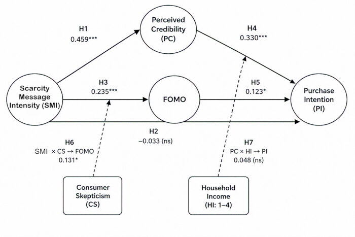
Figure 2: Structural model path coefficients. Standardized path coefficients (β) are shown for the direct (H1–H5) and moderating effects (H6–H7) in the final analytical sample (N = 272). Solid arrows indicate direct relationships, and dashed arrows indicate moderating effects. H1 and H6 were not supported because the statistically significant relationships were in the directions opposite to those hypothesized; H2 and H7 were not supported because the corresponding effects were not statistically significant; and H3–H5 were supported. SMI = Scarcity Message Intensity; PC = Perceived Credibility; PI = Purchase Intention; FOMO = fear of missing out; CS = Consumer Skepticism; HI = Household Income; ns = not significant. *p < 0.05; ***p < 0.001. Please click here to view a larger version of this figure.

Robustness Checks

Robustness checks were conducted to assess whether the findings were stable with respect to potential methodological and model-related concerns. Four complementary procedures were undertaken: (i) assessment of common method bias, (ii) diagnosis of multicollinearity, (iii) determination of effect sizes for the structural relationships, and (iv) assessment of the predictive relevance and explanatory power of the structural model.

Common Method Bias

Common method bias was assessed using Harman’s single-factor test in IBM SPSS Statistics (version 26). The first factor accounted for 31.70% of the total variance, which was below the 50% criterion applied in this study. The extracted factors collectively accounted for 65.50% of the total variance (Table 9). These results indicate that no single factor accounted for the majority of the variance, suggesting that common method bias was unlikely to substantially affect the findings.

Indicator	Value	Threshold	Conclusion
Total variance explained	65.50%	—	—
Variance explained by the first factor	31.70%	<50%	No serious common method bias

Table 9: Harman’s Single-Factor Test for Common Method Bias.

The total variance explained was 65.50%, while the first factor accounted for 31.70% of the variance. Because the variance explained by the first factor was below the 50% threshold, the test indicated no serious common method bias in the final analytical sample (N = 272).

Multicollinearity Diagnosis and Effect Sizes (f²)

Excessive multicollinearity among predictor constructs can inflate standard errors and destabilize path coefficients. VIF values were examined for the predictors in the structural model, and f² values were used to assess the effect sizes of the structural relationships.

As shown in Table 10, all predictor-level VIF values ranged from 1.000 to 1.366, well below the threshold of 3.00, indicating no problematic multicollinearity among the predictors. Regarding effect sizes, Scarcity Message Intensity → Perceived Credibility showed a medium effect (f² = 0.225). Scarcity Message Intensity → FOMO (f² = 0.142), Consumer Skepticism → FOMO (f² = 0.082), Perceived Credibility → Purchase Intention (f2 = 0.120), FOMO → Purchase Intention (f² = 0.047), and Scarcity Message Intensity → Purchase Intention (f² = 0.034) showed small effects. The H6 interaction showed a small effect (f² = 0.023), whereas Household Income (f² = 0.001) and the H7 interaction (f² = 0.003) showed negligible effects. Overall, the results indicate acceptable collinearity and varying effect sizes across the structural relationships.

Dependent Construct	Predictor Construct/Path	Predictor VIF	f²	Effect Size Rating
Perceived Credibility	Scarcity Message Intensity	1.000	0.225	Medium
FOMO	Scarcity Message Intensity	1.116	0.142	Small
FOMO	Consumer Skepticism	1.120	0.082	Small
FOMO	Scarcity Message Intensity × Consumer Skepticism (H6)	1.006	0.023	Small
Purchase Intention	Scarcity Message Intensity	1.366	0.034	Small
Purchase Intention	Perceived Credibility	1.311	0.120	Small
Purchase Intention	FOMO	1.310	0.047	Small
Purchase Intention	Household Income	1.005	0.001	Negligible
Purchase Intention	Perceived Credibility × Household Income (H7)	1.011	0.003	Negligible

Table 10: Collinearity and Effect-Size Assessment.

Predictor-level variance inflation factor (VIF) and f² effect-size values are reported for the final analytical sample (N = 272). VIF values <3.00 indicate acceptable collinearity. Effect sizes were classified as negligible (f² <0.02), small (0.02 to <0.15), medium (0.15 to <0.35), or large (≥0.35). Values represent regression-based checks using the final composite-score model. FOMO = fear of missing out.

Predictive Relevance (Q²) and Explanatory Power (R²)

The structural model’s explanatory power was evaluated using the coefficient of determination (R²), while predictive relevance was assessed using the Stone–Geisser Q² statistic obtained through the blindfolding procedure in SmartPLS 4.0 with an omission distance of D = 7.

As shown in Table 11, the model explained 21.3% of the variance in Perceived Credibility (adjusted R² = 0.210), 18.6% in FOMO (adjusted R² = 0.177), and 51.2% in Purchase Intention (adjusted R² = 0.503). All Stone–Geisser Q² values were greater than zero (0.145, 0.119, and 0.341, respectively), indicating predictive relevance for all three endogenous constructs.

Endogenous Construct	R2	Adjusted R2	Q2 (Stone–Geisser)	Predictive Relevance
Perceived Credibility	0.213	0.210	0.145	Yes (>0)
FOMO	0.186	0.177	0.119	Yes (>0)
Purchase Intention	0.512	0.503	0.341	Yes (>0)

Table 11: Explanatory Power and Predictive Relevance of the Structural Model.

R² and adjusted R² values indicate the proportion of variance explained in each endogenous construct. Stone–Geisser Q² values assess predictive relevance, with values >0 indicating predictive relevance. Results are reported for the final analytical sample (N = 272). FOMO = fear of missing out.

Data Availability Statement:

The de-identified item-level dataset for the 272 adult participants included in the final analysis is provided in Supplementary Data File 1. The dataset includes demographic variables, item-level responses, composite construct scores, and interaction terms used in the analysis. Likert-scale items are coded from 1 to 5. Household Income is included separately as a four-category demographic variable (1–4), while IL1–IL3 represent Financial Literacy/Financial Capability items and are distinct from Household Income. Financial Literacy/Financial Capability was not included as a latent construct in the final structural model. The complete bilingual study questionnaire, including the English and Simplified Chinese items, response scales, demographic questions, and coding instructions, is provided in Supplementary Data File 2.

Supplementary Data File 1: De-identified Dataset.

De-identified item-level dataset for the 272 adult participants included in the final analysis. The file contains demographic variables, item-level responses, composite scores, and interaction terms. Likert-scale items are coded from 1 to 5. Household Income is included separately as a four-category demographic variable coded from 1 to 4. IL1–IL3 represent Financial Literacy/Financial Capability items and are distinct from Household Income; Financial Literacy/Financial Capability was not included as a latent construct in the final structural model. Composite scores were calculated from their corresponding construct items, and interaction terms were calculated from the relevant mean-centered variables. Please click here to download this file.

Supplementary Data File 2: Study Questionnaire.

Complete bilingual study questionnaire containing the English and Simplified Chinese items used for data collection, together with response scales and coding instructions. The file includes demographic screening questions and items assessing Ad Engagement/Awareness, fear of missing out (FOMO), Scarcity Message Intensity, Perceived Credibility, Financial Autonomy, Purchase Intention, Financial Literacy/Financial Capability, and Consumer Skepticism. Likert-scale items were rated from 1 = Strongly Disagree to 5 = Strongly Agree. Household Income was recorded separately as a four-category demographic variable. Please click here to download this file.

讨论

The present study tested a dual-pathway model in which Scarcity Message Intensity is associated with Purchase Intention through an affective pathway involving FOMO and a cognitive pathway involving Perceived Credibility, with Consumer Skepticism and Household Income examined as moderators. Scarcity Message Intensity was positively associated with FOMO (β = 0.235, p < 0.001), supporting H3. Perceived Credibility (β = 0.330, p < 0.001) and FOMO (β = 0.123, p = 0.024) were also positively associated with Purchase Intention, supporting H4 and H5. In contrast, the direct association between Scarcity Message Intensity and Purchase Intention was not significant (β = −0.033, p = 0.569), and H2 was not supported. Both indirect effects were significant through Perceived Credibility (β = 0.151, p < 0.001) and FOMO (β = 0.029, p = 0.028), with a significant total indirect effect (β = 0.180, p < 0.001). These findings extend prior research on scarcity-driven consumer responses and FOMO^4,9,17,24by demonstrating that scarcity messaging can be associated with both affective and cognitive processes. The stronger indirect effect through Perceived Credibility (0.151) than through FOMO (0.029) suggests that cognitive appraisal was particularly prominent in this sample. This finding is consistent with research emphasizing the importance of credibility, advertising evaluation, and consumer skepticism in responses to marketing communications^{5,14,26,27,30}. Accordingly, the proposed model contributes by integrating cognitive and affective pathways rather than treating scarcity as a unitary stimulus that uniformly increases Purchase Intention.

A notable finding was the positive association between Scarcity Message Intensity and Perceived Credibility (β = 0.459, p < 0.001), contrary to H1. One possible explanation is product perishability. In fresh-fruit e-commerce, scarcity cues may signal high demand and rapid inventory turnover, which consumers may associate with freshness and product quality. This interpretation is consistent with Signaling Theory and research showing that scarcity effects depend on product and message characteristics^11,14,25. Participants’ recent experience purchasing fresh fruit online may also have helped them evaluate the plausibility of scarcity claims. Moreover, repeated exposure to urgency cues on Chinese social commerce platforms may normalize such signals as routine features of online shopping rather than inherently manipulative messages. These explanations remain theoretical and require further empirical investigation. The potential role of algorithmic literacy is relevant; however, because platform experience and algorithmic literacy were not directly measured, this explanation requires further empirical testing. More broadly, social media advertising has been associated with business outcomes such as visibility, customer engagement, and sales performance³¹. The interpretation of scarcity information as a quality-relevant signal is also consistent with cue-utilization theory, whereby consumers use available informational cues to infer product quality³². Together, product perishability, category familiarity, and platform-based cues may help explain why the cognitive pathway differed from the negative relationship predicted in H1.

The moderation findings further refine the dual-pathway framework. Consumer Skepticism moderated the relationship between scarcity message intensity and FOMO, but the observed effect was positive rather than the negative effect hypothesized in H6; therefore, H6 was not supported. This unexpected pattern suggests that skepticism may not necessarily protect consumers from scarcity-induced emotional responses. Instead, skeptical consumers may scrutinize persuasive cues more closely, consistent with the persuasion knowledge model and psychological reactance theory^12,13. Because these mechanisms were not directly measured, this interpretation requires further empirical testing. Rather than immediately dismissing an urgency message, skeptical consumers may scrutinize its persuasive intent more closely, potentially increasing attention to the scarcity cue^12,13. Consumer skepticism has similarly been shown to shape how consumers evaluate marketing claims and persuasive information³⁰. Such scrutiny may increase the salience of a potential missed opportunity, providing one possible explanation for the observed positive moderation effect. However, attentional elaboration and related psychological processes were not directly measured and should therefore be treated as theoretical interpretations rather than established mechanisms. The findings suggest that skepticism may not function solely as a defensive filter; under some conditions, greater scrutiny of persuasive intent may coexist with heightened FOMO.

The second moderation effect was not statistically significant. Household Income did not significantly moderate the relationship between Perceived Credibility and Purchase Intention (β = 0.048, p = 0.362); therefore, H7 was not supported. This finding suggests that the positive relationship between Perceived Credibility and Purchase Intention did not vary significantly across household income levels in the present sample. Although socioeconomic resources may influence consumer decision-making, the present findings do not provide evidence that Household Income systematically strengthens the effect of credibility on Purchase Intention. Accordingly, interpretations concerning greater financial latitude, shopping expertise, or quality sensitivity among higher-income consumers should not be inferred from these data. More broadly, the findings suggest that the affective and cognitive pathways may operate differently across consumer characteristics. Consumer Skepticism showed an unexpected positive moderating pattern in the scarcity–FOMO relationship, whereas Household Income did not significantly moderate the relationship between Perceived Credibility and Purchase Intention. Cultural context may also shape responses to scarcity cues. In social-commerce environments where social information and urgency cues are common, consumers may interpret indicators of demand and availability differently depending on their social and cultural context. However, these cultural mechanisms were not directly measured and should be examined in future cross-cultural research.

Several limitations qualify these findings. First, the cross-sectional design identifies associations but cannot establish causality or temporal ordering. Future experimental studies could manipulate scarcity intensity, authenticity, type, and product perishability, while longitudinal research could examine how repeated exposure to scarcity cues influences credibility, skepticism, FOMO, and Purchase Intention over time. Second, reliance on self-reported data creates potential common method bias, although Harman’s single-factor test showed that the first factor accounted for only 31.70% of the variance. Future research could incorporate behavioral measures, purchase records, or experimentally observed choices. Third, purposive recruitment of consumers with recent online fresh-fruit purchasing experience increases contextual relevance but limits generalizability to less digitally engaged or offline consumers. The demographic composition of the sample also limits broader generalization. Fourth, recruitment across multiple Chinese social-commerce platforms was not designed to permit platform-specific comparisons, although scarcity cues may operate differently across short-video, product-review, and live-streaming environments. Fifth, the findings are specific to fresh fruit, where perishability may give scarcity cues informational value that may not generalize to durable products. Finally, several proposed explanatory mechanisms including algorithmic literacy, perceived scarcity authenticity, product-category expertise, cultural orientation, and quality sensitivity were not directly measured. Future studies should operationalize these mechanisms and test their roles directly.

This study provides evidence that scarcity messaging in fresh-fruit social commerce is associated with both cognitive and affective pathways. Although Scarcity Message Intensity did not directly predict Purchase Intention, significant indirect effects through Perceived Credibility and FOMO highlight the importance of these psychological mechanisms. The unexpected positive relationship between scarcity intensity and credibility further suggests that scarcity cues may carry informational value in perishable-product contexts. Consumer Skepticism also showed an unexpected moderation pattern, whereas Household Income did not significantly moderate the credibility–purchase intention relationship. The model explained 21.3% of the variance in Perceived Credibility, 18.6% in FOMO, and 51.2% in Purchase Intention, with positive Q² values indicating predictive relevance. Overall, the findings support a dual-pathway perspective in which scarcity cues may function not only as urgency triggers but also as credibility- or quality-related signals. Future research should test these mechanisms across different products, consumer groups, cultural settings, and digital platforms, particularly by distinguishing authentic from manufactured scarcity and perishable from non-perishable products.

材料

本文使用的材料清单

姓名	公司	目录编号	评论
Consumer Skepticism Scale	Adapted from Obermiller and Spangenberg30	N/A	N/A
Consumer Skepticism Scale	Adapted from Obermiller and Spangenberg30	N/A	N/A
Fear of Missing Out (FOMO) Scale	Adapted from Przybylski et al.19	N/A	N/A
Fear of Missing Out (FOMO) Scale	Adapted from Przybylski et al.19	N/A	N/A
Household Income	Self-reported demographic variable	N/A	N/A
Household Income	Self-reported demographic variable	N/A	N/A
IBM SPSS Statistics, version 26	IBM Corp., Armonk, NY, USA	N/A	N/A
IBM SPSS Statistics, version 26	IBM Corp., Armonk, NY, USA	N/A	N/A
Perceived Credibility Scale	Adapted from MacKenzie and Lutz26 and Pornpitakpan27	N/A	N/A
Perceived Credibility Scale	Adapted from MacKenzie and Lutz26 and Pornpitakpan27	N/A	N/A
Purchase Intention Scale	Adapted from Dodds et al.28 and Spears and Singh29	N/A	N/A
Purchase Intention Scale	Adapted from Dodds et al.28 and Spears and Singh29	N/A	N/A
Scarcity Message Intensity Scale	Adapted from Gierl and Huettl25	N/A	N/A
Scarcity Message Intensity Scale	Adapted from Gierl and Huettl25	N/A	N/A
SmartPLS 4.0	SmartPLS GmbH, Oststeinbek, Germany	N/A	N/A
SmartPLS 4.0	SmartPLS GmbH, Oststeinbek, Germany	N/A	N/A