Machine Learning and Post-Hoc Feature Attribution for Predicting Cardiac MRI Motion Artifacts: A Retrospective Cohort Study

摘要

This study develops an interpretable machine learning framework to predict anxiety-induced motion artifacts during non-sedated cardiac magnetic resonance imaging. The goal is to provide individualized risk stratification to guide targeted nursing interventions and optimize preemptive resource allocation.

摘要

Anxiety-induced motion artifacts frequently compromise image quality during non-sedated cardiac magnetic resonance imaging (CMR), leading to rescans and increased healthcare burdens. This retrospective cohort study hypothesized that combining multidimensional psychological and physiological indicators could accurately predict artifact occurrence. Baseline data from 514 adult patients, encompassing 15 clinical features, were systematically analyzed. Four machine learning algorithms were trained and evaluated using the area under the receiver operating characteristic curve (AUC). The eXtreme Gradient Boosting model demonstrated the highest discriminative ability (AUC = 0.875). To provide clinical transparency, SHapley Additive exPlanations (SHAP) analysis was applied, revealing that state anxiety (evaluated via the State-Trait Anxiety Inventory State subscale, STAI-State), maximum breath-hold duration, and heart rate variability were primarily associated with artifact risk. The novelty of this approach lies in uncovering non-linear threshold effects—such as a sharp risk escalation when STAI-State scores exceeded 45—and complex interactions between physical capacity and claustrophobia. In conclusion, this interpretable machine learning framework offers a robust tool for patient-specific risk stratification, suggesting that preemptive and targeted nursing interventions could be optimized based on individualized algorithmic predictions.

引言

Although CMR is an important diagnostic tool, its long acquisition times and repeated instructions to hold breath make it difficult to use and depend on the patient's ability to cooperate well¹. The enclosed environment and sound of the scanner can often cause psychological stress and anxiety in non-sedated clinical environments². This anxiety is one of the main sources of patient's movement, which usually leads to motion artifacts. Such artifacts can result in poor image quality, require rescanning of sequences, and ultimately drive up the cost of healthcare³. Thus, the early detection of patients who are prone to motion artifacts due to anxiety is an important problem for radiologic nurses.

The current pre-operative nursing evaluations are predominantly dependent on the traditional linear measurement tools, including subjective judgment of clinical phenomena or unidimensional psychological questionnaires such as the State-Trait Anxiety Inventory (STAI)⁴. These methods are useful for providing baseline data, but may not adequately reflect the more complex physiological and psychological coupling that patients may have. Multiple factors, including level of emotional state, regulation of the autonomic nervous system, as well as physical factors like abdominal girth and maximum breath holding time, seem to influence whether or not motion artifacts occur⁵. However, these non-linear relationships and complex interactions between features are often hard to capture using traditional statistical methods and are therefore not well suited for precision nursing decision making^6,7.

Machine learning has been shown to have some promise in dealing with multi-dimensional clinical data and in identifying underlying non-linear patterns^8,9. In this study, the objective is to create predictive models for the risk of anxiety-induced motion artifacts, with the help of several machine learning algorithms, from routine pre-scan clinical indicators. In addition, the transparency of the predictive algorithms will be improved by SHAP analysis. This study aims to transform the algorithmic insights into an interpretable risk stratification framework to offer a data-driven reference point for targeted nursing interventions and interpretation of the potential non-linear thresholds and interactive effects among baseline features.

方案

Study design and ethical considerations
All equipment, hardware devices, measurement instruments, assessment scales, open-source R libraries, and analytical resources utilized in this study are comprehensively itemized in the Table of Materials. The overall experimental and analytical workflow is illustrated in Supplementary Figure 1. The study was an observational cohort study, in compliance with the ethical guidelines of the Declaration of Helsinki, as revised in 1975. This study protocol was approved by the Institutional Review Board of The Third People's Hospital of Chengdu (Approval No. 2026-S-143). Due to the observational nature of the study, which involved the extraction of anonymized clinical data from these patients in a retrospective fashion during routine clinical practice, the need for written informed consent was formally waived by the ethics committee. Data for patients from January 2019 to December 2025 were analyzed systematically.

Patient selection criteria
The study population included adult patients who were referred for non-sedated CMR. Inclusion criteria were as follows: (1) age ≥ 18 years; and (2) preoperative physiological and psychological assessment was completed. Patients were excluded if they had any of the following: (1) missing clinical baseline data; (2) severe arrhythmia (e.g., persistent atrial fibrillation [AF]); (3) cognitive dysfunction, severe hearing loss, or a language barrier to understanding breath-holding instructions; or (4) use of any sedative or anxiolytic drugs within 24 hours of the scan. Patient Preparation and Nursing Workflow: A standardized nursing workflow was implemented for all participants. Upon arrival, approximately 30 min prior to the scan, patients received detailed verbal instructions regarding the examination process, scanner noise, and the importance of remaining motionless. Anxiety assessments and baseline physiological measurements were conducted in a quiet preparation room. Subsequently, structured breath-hold training was administered by the radiologic nurse, requiring the patient to practice end-expiratory breath-holds following a voice command. During positioning, patients were placed supine on the scanner table, fitted with hearing protection (earplugs and headphones), and provided with an emergency squeeze ball. Two-way audio communication and visual monitoring via a camera were maintained consistently throughout the entire scanning procedure.

Data collection and clinical features
Fifteen baseline clinical indicators were systematically collected before the imaging process. Demographic variables such as age (in years) and gender were obtained from medical records, while education (in years) was self-reported by the patient during the nursing interview. Physiological parameters measured in the preparation room included resting heart rate (bpm), heart rate variability (HRV, ms) derived from a 5-min pre-scan ECG recording, maximum breath-hold duration (seconds) assessed during the training phase, systolic blood pressure (SBP, mmHg) measured using an automatic digital upper-arm blood pressure monitor, and peripheral oxygen saturation (SpO₂, %). Physical and medication parameters included abdominal girth (cm) measured at the umbilical level in the supine position using an ergonomic non-elastic medical circumference measuring tape, modified Mallampati score (class I-IV) assessed by clinical staff, and current use of beta-blockers extracted from electronic pharmacy records. Experiential factors, including history of claustrophobia and prior MRI experience, were determined via direct patient questioning and cross-verification with electronic medical records. Specifically, psychological stress was evaluated using the validated Chinese version of the STAI-State subscale (Form Y-1). This self-report questionnaire consists of 20 items rated on a 4-point Likert scale, yielding a total STAI-State score ranging from 20 to 80, where higher scores suggest greater acute anxiety. The assessment was administered by a trained nurse 30 min prior to the patient entering the scanner room. The full STAI questionnaire utilized in this study is provided in Supplementary File 1. In addition, the estimated scan time (min) was calculated theoretically based on the specific clinical protocol prescribed by the referring physician. The main outcome was the presence of motion artifacts due to anxiety requiring rescanning of sequences and/or significantly affecting the diagnostic image quality. Image quality was evaluated on the short-axis and long-axis cine sequences using a standard 4-point Likert scale: 1 (non-diagnostic, severe blurring), 2 (poor, moderate blurring affecting margin sharpness), 3 (good, mild blurring not affecting diagnosis), and 4 (excellent, no motion). The diagnostic threshold for an acceptable image was set at a score of 3 or higher. Cases scoring 1 or 2 due to motion were classified as having positive artifacts. The grading was independently performed by two cardiovascular radiologists, each with over five years of experience, who were blinded to the patients' clinical and psychological data. Any discrepancies in grading were resolved through consensus mediated by a senior radiologist with over ten years of experience. All imaging procedures were performed using a 3.0 T whole-body magnetic resonance scanner equipped with an 18-channel phased-array body coil and a 32-channel spine matrix coil. The standardized cardiac protocol included retrospectively electrocardiogram-gated steady-state free precession sequences for cardiac cine imaging. The typical acquisition parameters for cine imaging were as follows: repetition time of 3.4 ms, echo time of 1.4 ms, flip angle of 50°, slice thickness of 8 mm with a 2 mm gap, and an in-plane spatial resolution of 1.9 x 1.9 mm. Patients were required to hold their breath in expiration for approximately 10–15 s per slice acquisition.

Machine learning algorithms and class imbalance strategy
The data set was then split randomly into 70% training and 30% testing sets for building the predictive framework. Specifically, a fixed random seed (set.seed(123)) was utilized to ensure computational reproducibility. A stratified random sampling approach based on the outcome variable was employed to maintain the native class distribution across both subsets, resulting in a training set of 360 patients and a testing set of 154 patients. Four machine learning algorithms were tested: logistic regression, support vector machine (SVM), random forest and eXtreme Gradient Boosting (XGBoost). XGBoost model was chosen as the main analytical method because it is able to handle non-linear relationships and complex interactions. The XGBoost model was trained with the following hyperparameters: max_depth = 4, eta = 0.05, nrounds = 150 and objective function = binary:logistic. To rigorously prevent data leakage and evaluate true out-of-sample generalizability, all data preprocessing, hyperparameter selection, and decision threshold optimizations were strictly executed within the training set (n = 360). All reported model performance metrics, confusion matrices, calibration assessments, and decision curves were subsequently evaluated on the completely unseen, independent testing dataset (n = 154). In terms of class distribution, the outcome variable had a fairly even native proportion in regard to this particular cohort. As a result, it was decided not to use aggressive synthetic oversampling techniques. To avoid this, the decision threshold was adapted to the maximization of the F1-score and Youden's Index to achieve an optimal balance between precision and recall when classifying in the clinical environment.

Statistical analysis
Normally distributed continuous variables were reported as mean with standard deviation (SD) whereas non-normally distributed continuous variables were reported as median and interquartile range [IQR]. The data of categorical variables were presented as frequencies and percentages. Student's t test, Mann Whitney U test, Chi square or Fisher's exact test were used for baseline group comparisons as appropriate. The AUC and area under the precision-recall curve (AUPRC) were used to evaluate the discriminative performance of the models. Models were compared using the DeLong test to find the AUC differences. SHAP analysis was used to assess feature importance, feature dependence and feature interactions. The reliability of predicted probabilities was determined using calibration curves and Hosmer-Lemeshow testing (implemented via the hoslem.test function in the ResourceSelection package). Non-linear trend analysis and inflection derivatives were computed using local polynomial regression fitting (stats::loess in base R). Individual conditional expectation (ICE) trajectories were extracted via the shapviz package. Decision curve analysis (DCA) and clinical impact curves (CIC) were calculated and visualized using custom vectorized R functions adapted from the rmda methodology. R software and its associated packages (xgboost; pROC) were used for all statistical analyses. All data dictionaries, R analysis scripts, and model codes utilized in this study are provided in Supplementary File 2 to facilitate methodological reproduction. Statistically significant values were set at a p-value of < 0.05 (two-tailed).

结果

Baseline characteristics and exploratory data analysis
This study included 514 patients who had non-sedated CMR. Of these, 309 patients (60.1%) had motion artifacts due to anxiety. Demographic variables such as gender, education level and SpO₂ were not statistically different between the two groups, and therefore provided a similar baseline for subsequent analyses, as detailed in Table 1. To assess potential multicollinearity prior to extensive comparative analysis, a correlation matrix of the included clinical features was created (Figure 1A). Physiological relationships were found as expected, such as a negative correlation between HRV and resting heart rate, but no extreme collinearity was detected, indicating that severe linear multicollinearity was absent and the candidate features provided non-redundant linear information suitable for downstream multivariate modeling. Group comparisons revealed significant differences in core psychological and physiological measures. Patients in the artifact group presented with a higher state anxiety (STAI score) level compared to the non-artifact group (Figure 1B). Objective physiological parameters were also significantly altered, with the artifact group showing reduced heart rate variability (Figure 1C) and reduced maximum breath-hold duration (Figure 1D). Regarding previous MRI experience (Figure 1E), the univariate analysis showed a marginal P-value of 0.086; however, there was a trend toward a higher proportion of patients lacking previous MRI experience in the artifact group. Finally, exploratory analysis revealed that the probability of artifact occurrence exhibited a positive trend with increasing estimated scan duration (Figure 1F).

Machine learning model construction and performance evaluation
The exact sample sizes and the respective number of positive artifact cases for both the training (n = 360) and testing (n = 154) datasets are detailed in Supplementary Table 1, confirming that the native class distribution was evenly preserved across splits. Several machine learning algorithms were trained to predict anxiety-induced motion artifacts, building on the differences in baseline and non-linear trends found in exploratory data analysis. On the independent testing set (n = 154), the XGBoost model achieved an AUC of 0.875 (95% CI: 0.820–0.930), outperforming random forest (AUC = 0.822, 95% CI: 0.758–0.886), SVM (AUC = 0.805, 95% CI: 0.738–0.872), and logistic regression (AUC = 0.779, 95% CI: 0.708–0.850) (Figure 2A). Furthermore, on the precision-recall curve (Figure 2B), XGBoost achieved the highest AUPRC of 0.914, compared to 0.864 for random forest, 0.859 for SVM, and 0.833 for logistic regression. Comprehensive evaluation across multiple classification metrics on the test set (n = 154) demonstrated that XGBoost consistently achieved the highest overall performance: accuracy was 0.818 (95% CI: 0.758–0.878) for XGBoost, 0.768 (95% CI: 0.701–0.835) for random forest, 0.742 (95% CI: 0.672–0.812) for SVM, and 0.695 (95% CI: 0.623–0.767) for logistic regression. Sensitivity was 0.747 for XGBoost, 0.688 for random forest, 0.656 for SVM, and 0.593 for logistic regression. Specificity was 0.921 for XGBoost, 0.889 for random forest, 0.873 for SVM, and 0.841 for logistic regression. Positive predictive value (PPV/Precision) was 0.932 for XGBoost, 0.901 for random forest, 0.882 for SVM, and 0.844 for logistic regression. Negative predictive value (NPV) was 0.716 for XGBoost, 0.653 for random forest, 0.632 for SVM, and 0.589 for logistic regression. F1-score was 0.830 for XGBoost, 0.780 for random forest, 0.752 for SVM, and 0.697 for logistic regression (Figure 2C; Supplementary Table 2). Complete pairwise DeLong tests across all six model pairs revealed: XGBoost versus logistic regression (p = 0.041), XGBoost versus SVM (p = 0.089), XGBoost versus random forest (p = 0.162), random forest versus logistic regression (p = 0.312), SVM versus logistic regression (p = 0.540), and random forest versus SVM (p = 0.684) (Supplementary Table 3). This classification performance could be further highlighted by the confusion matrix for the optimal XGBoost model (Figure 2D). The model also had a high accuracy for predicting true positives and true negatives, but it is pointed out that 23 cases were predicted as negative but were actually artifacts. It could be due to erratic and abrupt patient motion or to transient discomfort during the lengthy scan and is intrinsically hard to capture completely with pre-scan baseline indicators.

The reliability of the predicted probabilities was tested with a calibration curve (Figure 2E). Often the curve followed the diagonal line of reference and the Hosmer-Lemeshow test showed a non-significant p-value of 0.163, suggesting no significant deviation from a perfect fit. Minor variations in the curve may be attributable to the natural variation in actual clinical situations. Lastly, DCA (Figure 2F) was used to assess clinical utility of the model. The XGBoost model exhibited a greater net clinical benefit over a wide spectrum of threshold probabilities than did the logistic regression model as well as the default strategies of treating all or no patients. This implies that it could be useful as an assistive device to inform targeted nursing interventions.

Global interpretability and non-linear associations via SHAP analysis
Once the predictive ability of the XGBoost model was validated, SHAP analysis was performed to understand the features that the model relied upon to make its predictions. It should be emphasized that the values for SHAP correspond to statistical relationships and the influence of features on the model output, but do not indicate causal relationships. Figure 3A is a SHAP summary plot showing the directional impact of the clinical variables on model predictions. For example, higher STAI scores and longer scan durations (shown as red dots) tend to be related to a higher probability of artifacts (indicated by positive SHAP values). In contrast, higher maximum breath-hold durations are concentrated on the negative side of the SHAP axis, indicating a negative attribution value associated with a reduced predicted probability of artifacts within the model structure. Consistently, the feature importance ranking (Figure 3B) indicated the STAI score, maximum breath-hold duration, estimated scan duration, and HRV as key features for predicting motion artifacts, aligning with the earlier noted baseline differences. In order to better understand the complex relationships obtained by the non-linear algorithm, SHAP dependence plots were created. The STAI-State score and predicted artifact probability demonstrated an empirical non-linear trajectory (Figure 3C). Mathematical evaluation of the LOESS curve's first and second derivatives, combined with tree split frequency analysis, identified an inflection zone around an STAI-State score of 45 (where SHAP values shifted from negative to sharply positive). However, this threshold should be interpreted as an empirical transition zone with inherent individual variation rather than a deterministic biological boundary. This pattern indicates a model-learned non-linear transition point, suggesting that while the algorithm attributes minimal incremental risk across lower anxiety scores, scores exceeding approximately 45 receive markedly higher positive SHAP attributions toward artifact prediction. To examine the dose-response relationship between acute anxiety levels and motion artifact incidence, patients were stratified across four established STAI-State clinical score bands: mild anxiety (<35, n = 165), moderate anxiety (35–44, n = 144), clinically significant elevated anxiety (45–54, n = 125), and severe anxiety (≥55, n = 80). The observed artifact occurrence rates exhibited a pronounced graded escalation: 21.2% (35/165) in the <35 group, 45.8% (66/144) in the 35–44 group, 82.4% (103/125) in the 45–54 group, and 94.6% (76/80) in the ≥55 group (trend p < 0.001). This graded relationship corroborates the non-linear risk escalation identified by post-hoc SHAP analysis around the score of 45, which aligns with published clinical thresholds designating clinically actionable situational anxiety.

As far as physiological parameters concerned, the shorter the maximum breath holding time, the more likely to be an artifact, and vice versa, the longer the breath holding time, the less the chance that the data were an artifact (Figure 3D). Likewise, reduced HRV was associated with positive SHAP values, further indicating that reduced autonomic regulation may be associated with increased risk (Figure 3E). A slight upward inflection at the extreme high values in the data distribution is noted in the LOESS smoothing curves in Figure 3D and Figure 3E. The latter is most likely a mathematical effect of the smoothing algorithm fitting the sparse, isolated data points at the ends, and not a change in actual physiology of risk. Lastly, there was a steady positive correlation between the estimated scan duration and the SHAP value (Figure 3F), suggesting that prolonged scan time serves as an important positive contributor to the model's prediction of motion artifacts.

Feature interactions and individualized risk trajectories
In addition to assessing the unique effects of clinical variables, SHAP interaction plots provided insights into how the XGBoost model captures interactions between variables which may be complex and multi-dimensional. There was an interaction between STAI score and previous MRI experience as shown in Figure 4A. Interestingly, patients with high STAI score (STAI score > 45) had obviously higher SHAP values than patients who had already had an MRI. This pattern indicates a model-learned interaction where prior exposure to the imaging environment is associated with an attenuation of the high positive SHAP attribution typically assigned to elevated situational anxiety within the algorithm.

Likewise, a possible synergy between the physiological capacity and physical attributes was found. At a shorter maximum breath-hold duration, the patients with larger abdominal girths tended to have higher SHAP values as shown in Figure 4B. This indicates that the algorithm assigns compounded positive attribution toward artifact prediction when limited breath-holding capacity coincides with increased abdominal dimensions. Another correlation was observed between autonomic regulation and psychological stress; among people with low HRV, high STAI scores were linked to even higher SHAP values, demonstrating a synergistic model attribution where the co-occurrence of reduced autonomic tone and high anxiety produces the highest positive contribution to predicted artifact probability within the model (Figure 4C). Further, longer estimated scan times yielded a more pronounced escalation in model-predicted risk among patients with a history of claustrophobia: at scan durations exceeding 50 min, the mean positive SHAP attribution reached +0.62 in claustrophobic patients compared to +0.28 in non-claustrophobic patients, indicating a distinct vulnerability within this subgroup during prolonged imaging (Figure 4D).

ICE curves were created to represent the trajectories of predicted probabilities, in order to translate these model-level insights into patient-specific risk assessment. Figure 4E illustrates the distribution of the predicted probability of the presence of motion artifacts for each patient in relation to his or her STAI score. The overall trend was that the mean predicted probability remained relatively stable across the lower score spectrum (hovering between 40.2% and 58.1% across STAI-State scores of 20 to 44), but escalated sharply from 58.1% to a plateau of 98.4% (individual range: 95.1%–99.8%) as scores surpassed the empirical inflection point of 45. The step-wise appearance of these trajectories is a mathematical property of tree-based machine learning algorithms that subdivide data at a finite number of split points, and does not necessarily indicate abrupt changes in biological state. The underlying gray lines representing the individual patients' baseline risk level also show the heterogeneity of the cohort in the vertical direction. The predicted probability decreased in a step-wise fashion as breath-hold duration increased, illustrating the model-predicted probability reduction associated with longer breath-hold duration across individual patient trajectories (Figure 4F).

Clinical application and risk stratification
SHAP waterfall plots were created for illustrative examples to showcase the practical use of the XGBoost model in clinical assessment of individuals. Figure 5A shows an “artifact probability” of 99.1% in a high-risk patient. In this particular case, the most important factors that increased the risk of a high score were a high STAI score and a brief breath-hold time. In contrast, Figure 5B shows that the low-risk profile has a projected event risk of 6.5% and is primarily due to good baseline characteristics. The important thing to note is that the x axis of these waterfall plots is the log-odds impact and not the absolute probability. This is a mathematical requirement to ensure additivity of the individual SHAP values and the final predicted probability is the transformed sum of the impacts.

The probability density distribution at the cohort level (Figure 5C) demonstrated distinct (although not absolute) separation in the scores predicted by the models for patients with and without the actual artifacts (p < 0.001). The reason for these overlaps may be due to the natural variation and noise of clinical practice. From these predicted probabilities, the cohort was divided into low, moderate and high clinical risk groups (Figure 5D). Artifact occurrence rates were actually in the correct order, with the high risk group having 93.6%. A small number of false positives (the remaining 6.4%) indicates that the model has some level of generalization, and is not overfitting the training data significantly.

A clinical impact curve was analyzed to further assess the practical implications of implementing this model (Figure 5E). For each level of risk, the predicted number of high-risk patients requiring intervention closely tracked the actual number of artifact cases: at the 40% risk threshold, 638 per 1,000 patients were predicted as high-risk compared to 586 true positive artifact cases, reflecting a modest false-positive margin of 5.2% (52/1,000). At the 50% threshold, 545 per 1,000 patients were predicted as high-risk versus 512 true positive cases (false-positive margin of 3.3%), demonstrating that algorithmic risk alerts maintain high specificity and minimize unwarranted preemptive nursing interventions across clinically relevant decision thresholds. Finally, based on the F1-score (Figure 5F), an optimization analysis found that 42% was the optimal intervention threshold to give the maximum F1-score of 0.940. This threshold could be one indicator that the nursing personnel may wish to consider when deciding how to allocate intervention resources and when a motion artifact needs to be avoided.

DATA AVAILABILITY:
The deidentified clinical dataset and the source data underlying the figures presented in this study have been permanently deposited in the Zenodo repository and are publicly available at https://doi.org/10.5281/zenodo.21980716.

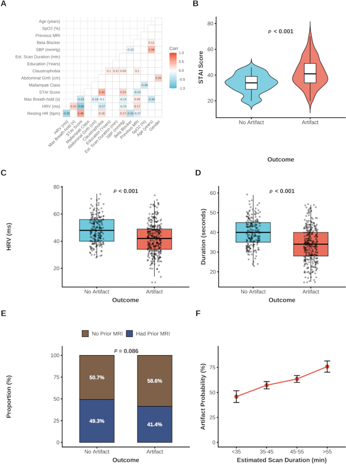
Figure 1: Data exploration and distribution of clinical characteristics. (A) Correlation matrix of the included clinical features. Colors indicate the correlation coefficients. (B) Distribution of STAI score in patients with and without motion artifacts. (C) Distribution of heart rate variability (HRV) in patients with and without motion artifacts. (D) Distribution of maximum breath-hold duration in patients with and without motion artifacts. (E) Proportion of patients with and without previous MRI experience in the two groups. (F) Trend of artifact probability across different estimated scan durations. Error bars represent standard errors. Please click here to view a larger version of this figure.

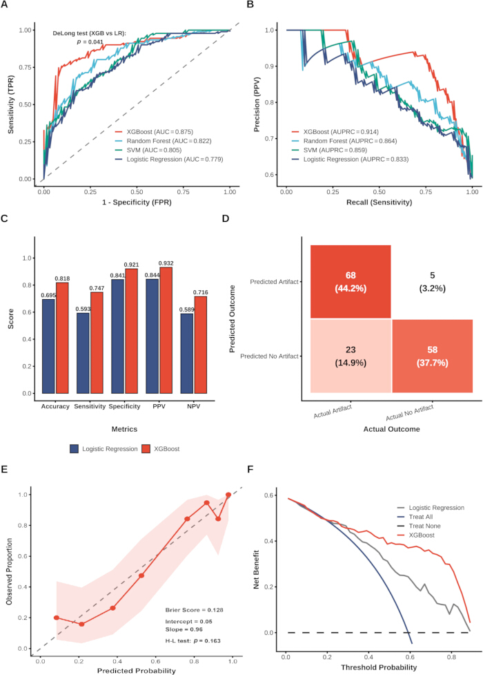
Figure 2: Performance evaluation of the machine learning models. (A) Receiver operating characteristic (ROC) curves of the evaluated models. The p-value from the DeLong test comparing XGBoost and logistic regression is shown. (B) Precision-recall curves of the evaluated models. (C) Comparison of key performance metrics between logistic regression and XGBoost. (D) Confusion matrix of the XGBoost model for predicting motion artifacts. (E) Calibration curve of the XGBoost model showing agreement between predicted probabilities and observed proportions. (F) DCA showing the net benefit of the models across a range of threshold probabilities. Abbreviations: AUC = area under the receiver operating characteristic curve; AUPRC = area under the precision-recall curve; FPR = false-positive rate; HR = heart rate; NPV = negative predictive value; PPV = positive predictive value; ROC = receiver operating characteristic; SVM = support vector machine; TPR = true-positive rate; XGBoost = eXtreme Gradient Boosting. Please click here to view a larger version of this figure.

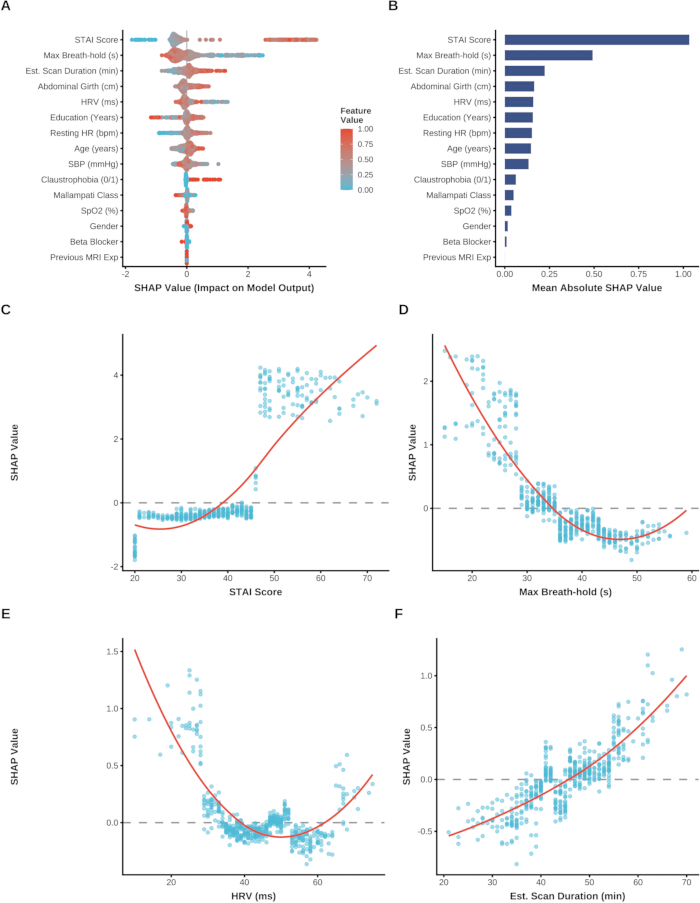
Figure 3: Global interpretability of the XGBoost model using SHAP analysis. (A) SHAP summary plot showing the distribution and direction of SHAP values for each feature. Colors indicate feature values, ranging from low (blue) to high (red). (B) Feature importance ranked according to the mean absolute SHAP value. (C) SHAP dependence plot for STAI score. (D) SHAP dependence plot for maximum breath-hold duration. (E) SHAP dependence plot for HRV. (F) SHAP dependence plot for estimated scan duration. Red lines represent LOESS smoothing curves illustrating potential nonlinear relationships between the features and model output. Abbreviations: HRV = heart rate variability; LOESS = locally estimated scatterplot smoothing; MRI = magnetic resonance imaging; SBP = systolic blood pressure; SHAP = SHapley Additive exPlanations; SpO₂ = peripheral oxygen saturation; STAI = State-Trait Anxiety Inventory; XGBoost = eXtreme Gradient Boosting. Please click here to view a larger version of this figure.

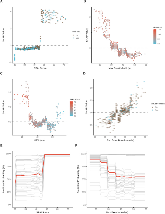
Figure 4: Feature interaction analysis and individual risk trajectories. (A) SHAP interaction plot showing the combined effects of STAI score and previous MRI experience on model output. (B) SHAP interaction plot showing the combined effects of maximum breath-hold duration and abdominal girth on model output. (C) SHAP interaction plot showing the combined effects of HRV and STAI score on model output. (D) SHAP interaction plot showing the combined effects of estimated scan duration and history of claustrophobia on model output. (E) ICE curves showing predicted probability trajectories for individual patients across varying STAI scores. (F) ICE curves showing predicted probability trajectories for individual patients across varying maximum breath-hold durations. Thick red lines represent the average trends. Abbreviations: HRV = heart rate variability; MRI = magnetic resonance imaging; SHAP = SHapley Additive exPlanations; STAI = State-Trait Anxiety Inventory. Please click here to view a larger version of this figure.

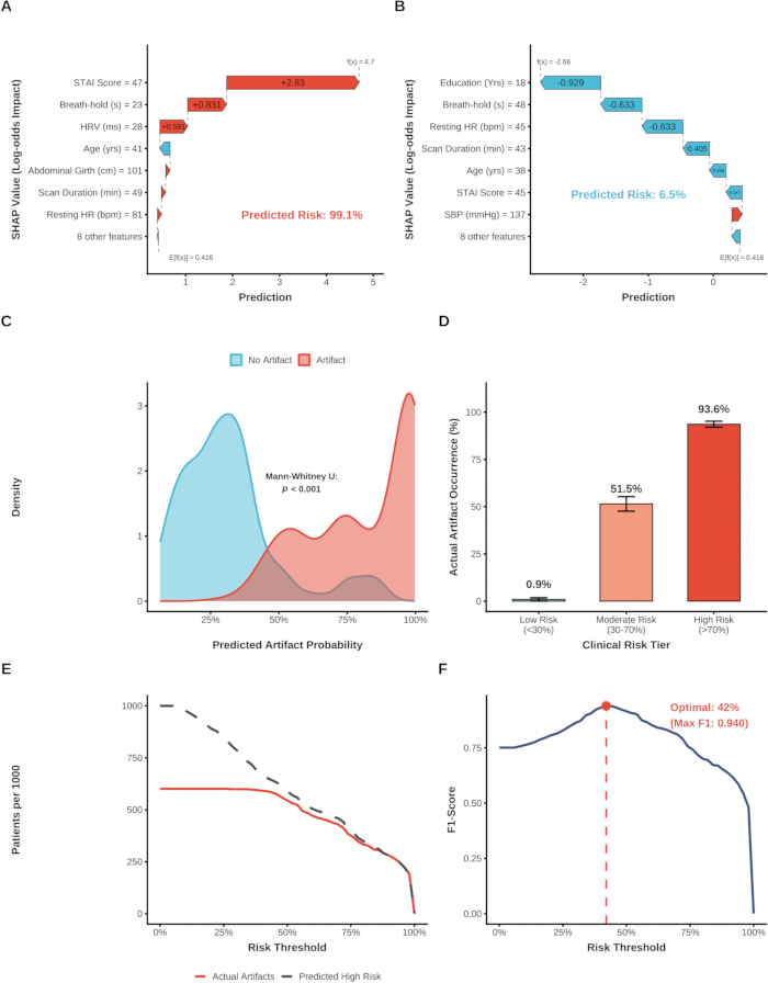
Figure 5: Clinical application and risk stratification based on the XGBoost model. (A) SHAP waterfall plot for a representative high-risk patient, showing the positive (red) and negative (blue) contributions of individual features to the prediction. (B) SHAP waterfall plot for a representative low-risk patient, showing the positive (red) and negative (blue) contributions of individual features to the prediction. (C) Probability density distributions of predicted artifact probabilities according to actual outcome. (D) Actual artifact occurrence rates across clinical risk categories (low, moderate, and high risk). (E) Clinical impact curve comparing the predicted number of high-risk patients with the actual number of artifact cases per 1,000 patients across different risk thresholds. (F) Optimization of the clinical intervention threshold, with the red point indicating the threshold that maximizes the F1-score. Abbreviations: HR = heart rate; HRV = heart rate variability; SBP = systolic blood pressure; SHAP = SHapley Additive exPlanations; STAI = State-Trait Anxiety Inventory; XGBoost = eXtreme Gradient Boosting. Please click here to view a larger version of this figure.

Supplementary Figure 1: Comprehensive workflow of the study. The diagram summarizes the overall study workflow, including patient selection, data collection, machine learning model development and evaluation, model interpretation, and clinical risk stratification. Please click here to download this file.

Table 1: Baseline clinical characteristics of the study population categorized by the occurrence of motion artifacts. Data are presented as mean (standard deviation) for normally distributed continuous variables, median [interquartile range] for nonnormally distributed continuous variables, and number (%) for categorical variables. The total sample size was N = 514 (no artifact, n = 205; artifact, n = 309). p-values were calculated using Student’s t-test for normally distributed continuous variables, the Mann–Whitney U test for nonnormally distributed continuous variables, and the chi-square test or Fisher’s exact test for categorical variables, as appropriate. Abbreviations: HR = heart rate; HRV = heart rate variability; IQR = interquartile range; MRI = magnetic resonance imaging; SBP = systolic blood pressure; SD = standard deviation; SpO₂ = peripheral oxygen saturation; STAI = State-Trait Anxiety Inventory. Please click here to download this Table.

Supplementary Table 1: Sample size distribution and class balance across the overall cohort, training set, and testing set. Data are presented as number (%). The dataset was partitioned using stratified random sampling based on motion artifact status with a fixed random seed (set.seed(123)). The p-value was calculated using Pearson’s chi-square test with Yates’ continuity correction to compare the proportion of motion artifact cases between the training and testing sets. Please click here to download this file.

Supplementary Table 2: Predictive performance of the evaluated machine learning models on the independent testing dataset. Performance metrics were calculated on the independent testing dataset (n = 154; 91 motion artifact cases and 63 non-artifact cases) using decision thresholds derived from the training set. The 95% confidence intervals (CIs) for AUC were calculated using 2,000 stratified bootstrap replicates, and 95% CIs for accuracy were calculated using the exact binomial (Clopper–Pearson) method. p-values were calculated using the DeLong test comparing each model with XGBoost. Abbreviations: AUC = area under the receiver operating characteristic curve; AUPRC = area under the precision-recall curve; CI = confidence interval; NPV = negative predictive value; PPV = positive predictive value; ROC = receiver operating characteristic; SVM = support vector machine; XGBoost = eXtreme Gradient Boosting. Please click here to download this file.

Supplementary Table 3: Pairwise statistical comparison of model discrimination using the DeLong test. Values represent p-values from pairwise DeLong tests comparing the receiver operating characteristic curves of XGBoost, random forest, support vector machine, and logistic regression. Abbreviations: ROC = receiver operating characteristic; XGBoost = eXtreme Gradient Boosting  Please click here to download this file.

讨论

Patient anxiety during non-sedated CMR leads to non-diagnostic motion artifacts in approximately 10% to 30% of unselected clinical cohorts and up to 60% in anxiety-prone populations, prolonging scan times by 15 to 20 min and substantially escalating institutional healthcare expenditures through repeat sequence acquisitions^10,11. This study created a machine learning model using XGBoost to predict the occurrence of these artifacts and used SHAP analysis to unveil the non-linear relationships and interaction effects of baseline psychological and physiological variables, offering a data-driven approach to risk stratification and targeted nursing interventions.

However, previous studies have mainly focused on evaluating patient's compliance with imaging procedures using a psychological questionnaire that relies on a single index or a traditional linear regression model. The outcome of the present study however shows that the XGBoost model was able to produce better discriminative performances than the logistic regression^12,13. This enhancement indicates that the predictive relationships between baseline clinical indicators and motion artifact occurrence are multidimensional and non-linear within the dataset. The current sample size of the cohort is moderate for complex deep learning, but for tree-based ensemble algorithms, it is deemed as appropriate for detecting complex patterns in the data and interactions between features that are not captured by traditional parametric models¹⁴.

The SHAP analysis provided a detailed look at the contribution of the various features, with state anxiety, maximum breath-hold duration and heart rate variability being the major features associated with the risk of an artifact. It should be stressed here that the SHAP values are not the actual causal physiological pathways but rather statistical associations as per the logic of the model¹⁵. Interestingly, the dependence plots indicated that an empirical non-linear transition zone: positive SHAP attribution shifted sharply from −0.42 at an STAI-State score of 40 to +3.85 at scores exceeding 48. A consistent non-linear pattern was observed for breath-holding capacity (where SHAP attribution rose from -0.58 at durations >45 s to +2.48 at durations <20 s) and autonomic regulation (where SHAP attribution increased from −0.18 at HRV >50 ms to +1.28 at HRV <20 ms). There were some small variations, either at the high or low end of any of these distribution curves, but this is a normal mathematical feature that occurs when the smoothing algorithm is applied to sparse data at the margins and does not seem to detract from the broader clinically plausible trends¹⁶.

Moreover, the interaction analyses indicated that the high positive SHAP attribution of elevated anxiety was attenuated in patients with prior MRI experience, while larger abdominal girth compounded the model-predicted risk associated with shorter breath-hold capacity. A risk stratification scheme and clinical impact curve analysis were used to transform these algorithmic insights into clinical guidance for nursing. This is because, in the real world, clinical environments have natural noise and inter-individual variability, and the high-risk class naturally achieved a 93.6% occurrence rate, which is not an absolute maximum, but rather a realistic figure that demonstrates good generalization while preventing overfitting. The optimized intervention threshold obtained from this study could be used by the nursing personnel to effectively utilize the preemptive resources, balancing between failure in scan and unnecessary intervention of patients. When considering alternative methodologies, traditional clinical risk scoring systems offer simplicity but often fail to capture the synergistic effects elucidated by our model. Alternatively, incorporating intra-scan physiological tracking (such as real-time respiratory belts or functional continuous ECG monitoring) could provide a dynamic assessment of anxiety and impending motion, potentially offering a time-series alternative to static baseline predictions. Ultimately, transitioning from this retrospective design to a prospective multicenter validation approach will be essential to comparatively evaluate whether ML-driven predictions yield superior patient outcomes compared to standard nursing intuition. In summary, this study provides three principal contributions relative to existing literature: First, from a methodological perspective, it addresses the limitation of unidimensional pre-scan screening by demonstrating that coupling objective autonomic metrics (HRV) and physical capacity (breath-hold) with acute psychological scores (STAI-State) via tree-based algorithms significantly improves artifact prediction accuracy. Second, from a clinical translation standpoint, post-hoc feature attribution successfully transforms abstract algorithmic probabilities into transparent risk strata with an empirically optimized 42% intervention threshold, providing radiology nurses with a concrete decision-support tool. Third, to enable practitioners and researchers to build upon, validate, and adapt this framework, our complete analytical code, data dictionary, and anonymized dataset have been made publicly accessible as an open-source pipeline (Supplementary File 2). Nonetheless, as our findings originate from a single-center cohort, prospective external validation across diverse healthcare systems remains an essential prerequisite before broad clinical implementation.

There are some limitations in this study. Firstly, artifact grading inherently relies on subjective visual assessment by radiologists, and despite establishing blinded consensus protocols, minor evaluation biases may persist. Secondly, the sample size of 514 patients is relatively constrained for complex machine learning. While measures such as fitting preprocessing pipelines solely on the training set were employed to prevent data leakage, and a validation set was utilized to monitor potential overfitting, the robustness of the model could be further stabilized with a larger dataset. Thirdly, this investigation was largely a single-center study; institutional-specific factors like scanner bore size, ambient acoustic noise, and local patient preparation protocols could have an intrinsic impact on the results, highlighting the critical absence of, and need for, multicenter external validation. Lastly, the predictive model was built exclusively from baseline assessments, which may not adequately capture the dynamic physiological or psychological fluctuations patients undergo during extended scanning periods.

In conclusion, this study created an interpretable machine learning framework based on the XGBoost algorithm to forecast anxiety-induced motion artifacts in non-sedated cardiac MR imaging. Through SHAP analysis, possible non-linear relationships and interactions between psychological status, physiological ability, and physical traits were found. Interestingly, a specific threshold effect of state anxiety was identified. While the clinical implications of these algorithmic results suggest the possibility of tailoring nursing interventions using optimal probability thresholds to improve resource allocation, it must be explicitly clarified that the current model provides risk prediction only. Prospective randomized clinical trials are strictly required to confirm whether nursing interventions guided by these algorithmic risk scores translate into an actual reduction in artifacts and improved clinical efficacy.

材料

本文使用的材料清单

姓名	公司	目录编号	评论
18-channel body matrix coil	Siemens Healthcare	Body 18	Phased-array body matrix radiofrequency coil used for thoracic CMR signal reception
32-channel spine matrix coil	Siemens Healthcare	Spine 32	Integrated table spine coil used in combination with body coil during cardiac MRI
Automatic digital blood pressure monitor	Omron Healthcare	HEM-7121	Digital upper-arm sphygmomanometer used for pre-scan systolic blood pressure measurement
caret package	CRAN	Version 6.0-93	R library used for stratified data splitting and confusion matrix evaluation (RRID:SCR_021138)
Clinical dataset and analysis scripts	Zenodo	DOI: 10.5281/zenodo.21980716	Public repository containing deidentified patient data, modeling code, and DCA/CIC scripts
dplyr package	CRAN	Version 1.1.2	R package used for clinical data wrangling and transformation (RRID:SCR_016708)
e1071 package	CRAN	Version 1.7-13	R library used for Support Vector Machine (SVM) modeling (RRID:SCR_025345)
Emergency squeeze ball	Siemens Healthcare	Pneumatic Call Bulb	MR-safe pneumatic bulb for real-time patient-nurse emergency communication
ggplot2 package	CRAN	Version 3.4.2	R package used for publication-quality visual graphic rendering (RRID:SCR_014601)
Hearing protection headset and foam	Siemens Healthcare	MR Audio System	MR-safe acoustic noise attenuation system with pneumatic audio communication line
MAGNETOM Prisma 3.0 T MRI scanner	Siemens Healthcare	risma VE11C	Clinical 3.0 Tesla whole-body magnetic resonance imaging system
Medical circumference measuring tape	Seca GmbH	Seca 201	Ergonomic non-elastic medical measuring tape used for pre-scan abdominal girth assessment
patchwork package	CRAN	Version 1.1.2	R library used for combining multi-panel figures
pROC package	CRAN	Version 1.18.0	R package used for ROC curve analysis and DeLong statistical significance testing (RRID:SCR_022718)
PRROC package	CRAN	Version 1.3.1	R package used for Precision-Recall curve computation
Pulse oximeter and ECG monitoring unit	Siemens Healthcare	Wireless Physiological Unit	MR-compatible physiological monitoring unit for pre-scan SpO2, HR, and HRV recording
R software environment	R Foundation for Statistical Computing	Version 4.2.2	Core platform for machine learning and statistical computing (RRID:SCR_001905)
randomForest package	CRAN	Version 4.7-1.1	R library implementing Breiman's random forest algorithm for classification (RRID:SCR_015718)
ResourceSelection package	CRAN	Version 0.3-5	R library used for Hosmer-Lemeshow goodness-of-fit calibration testing
shapviz package	CRAN	Version 0.9.1	R library used for extracting SHAP values, beeswarm plots, and ICE trajectories
State-Trait Anxiety Inventory (STAI)	Mind Garden, Inc.	Form Y-1	Standardized 20-item self-report questionnaire assessing acute state anxiety levels
stats package (Base R)	R Core Team	Version 4.2.2	Built-in R package providing loess local polynomial regression and derivative modeling
tableone package	CRAN	Version 0.13.2	R library used for baseline demographic and statistical table synthesis
xgboost package	CRAN	Version 1.7.5.1	eXtreme Gradient Boosting algorithm used as the primary prediction framework (RRID:SCR_021361)