小鼠模型在推动我们对胚胎发育的理解方面发挥着关键作用。本文介绍了一种对完整固定的小鼠胚胎进行蛋白质和转录本染色的实验方案,以及如何在三维空间中对染色结果进行定量分析。这些技术可实现对关键发育细胞类型和发育过程的可视化与分析。
方法文章
优化的小鼠胚胎整体蛋白与转录表达发育研究方法
100 次观看
⸱
2026年9月11日
本文内容
摘要
摘要
小鼠模型在推动我们对胚胎发育的理解方面发挥了重要作用。分析胚胎内蛋白质和转录本的表达与定位,对于阐明发育和疾病相关的细胞与分子机制至关重要。然而,传统的小鼠胚胎转录本和蛋白质分析技术存在局限性。RNA 原位 杂交可实现转录本的整体染色,但缺乏多重检测能力。相比之下,胚胎切片技术虽可实现多重靶标染色,但仅限于二维(2D)层面。近年来,RNAscope 和免疫荧光染色等技术已被应用于整体胚胎,可在三维(3D)空间中实现多重靶标检测。这些方法能够在克服传统技术局限性的同时,对胚胎发育所必需的关键相互作用、信号通路和细胞类型进行定位与描绘。
本文介绍了使用RNAscope或免疫荧光法对固定后的胚胎第8.5天(E)8.5和E9.5小鼠胚胎进行整体染色的优化方法。两种方法均可在同一胚胎中同时实现最多4个靶标的多重检测。我们还提供了一种在同一胚胎中联合使用免疫荧光染色与RNAscope的方法,以可视化发育过程中蛋白质与转录本之间的相互作用。此外,我们描述了利用蔡司Arivis Pro软件对整个胚胎以及特定发育细胞类型中靶标表达进行共聚焦成像和三维分析的工作流程。综上所述,这些方法可实现对三维空间中多重蛋白质和转录本靶标的全面分析,为研究早期至中期胚胎发生过程中的细胞与分子相互作用提供了强有力的系统。
引言
小鼠模型在推动发育生物学研究进展方面发挥了重要作用,因其允许在体内(in vivo)研究与人类相关的发育过程,这得益于小鼠与人类在发育上的同源性,并可通过Cre-LoxP或CRISPR/Cas9等关键技术调控基因表达1,2。小鼠与人类之间约90%的基因组区域是保守的3,且两者共享许多发育过程。例如,小鼠和人类的胚胎发生均遵循相似的时间进程,包括受精卵形成、发育为胚泡,随后发生植入和原肠胚形成4。此外,大多数器官的发育在小鼠和人类之间也十分相似。例如,人类和小鼠心脏均经历相似的心脏环化、心房与心室的分隔、瓣膜形成以及流出道形成等过程,最终发育为四腔心脏5。因此,发育中及完全成熟的小鼠与人类心脏在结构上具有显著的相似性6,7。
为了研究正常和病理发育过程中发生的过程,已开发出多种技术,能够实现关键蛋白质和转录本的空间可视化。这些技术包括免疫荧光染色和RNA 原位杂交。
RNA 原位 杂交技术最早由 Gall 和 Pardue8 以及 John、Brinstall 和 Jones 于 1969 年9,以及 Buongiorno-Nardelli 和 Amaldi 于 1970 年10 首次描述。该技术用于检测转录本在组织中的表达8。简而言之,选择含有与目标 RNA 互补序列的探针,并用可检测的标记物进行标记。此类标记物包括放射性标记、生物素或地高辛。固定后的样品需进行通透处理,以允许探针渗透,随后探针与组织中的靶序列杂交。若使用放射性标记,可直接对组织成像;否则可通过与碱性磷酸酶或荧光染料偶联的抗体来可视化标记信号。RNA 原位 杂交的优势在于可用于整体样品染色,实现三维定位11。然而,该技术通常受限于多重检测能力,一般只能同时检测不超过两个目标,除非采用具有特定应用的优化技术,或使用 DNA 杂交方法(如用于染色体荧光标记的 M-FISH 技术)12,13。
免疫荧光技术由 Coons 等人于 1941 年首次开发14,15,是一种用于检测固定或冷冻样本中目标蛋白的方法。简而言之,样本 需先进行封闭处理,以减少抗体与组织非靶区域的非特异性结合。随后,将针对目标抗原的特异性一抗与样本孵育。一抗可直接与荧光染料或荧光蛋白偶联,也可通过使用荧光标记的二抗进行间接检测,该二抗特异性识别一抗所来源的物种。相比直接偶联荧光基团的一抗,使用二抗的优势在于可实现信号放大,从而提高检测灵敏度。通过使用不同物种来源的一抗,并结合直接偶联或与不同激发和发射光谱的荧光染料偶联的二抗,可实现多靶标同时检测。
传统的技术如RNA原位杂交和免疫荧光存在局限性。通常,RNA原位杂交仅允许在样品中检测单一靶标,因此不同细胞类型和通路之间的相互作用研究极为受限。此外,免疫荧光传统上是在组织切片中进行,而非整体封片,导致空间分辨率局限于二维。近年来的技术发展则聚焦于在三维系统中实现多重靶标检测。免疫荧光方案的优化使其可用于整体封片样品16。此外,已开发出可通过荧光标记探针实现转录本多重检测的技术,其原理与免疫荧光类似。
RNAscope 由 Wang 等人于 2012 年首次描述,其基于 RNA 原位 杂交技术17,可在固定样本中实现转录本的空间定位。简而言之,固定后的样本经过通透处理,使靶标探针能够渗入并与互补的转录序列结合。RNAscope 探针采用“双 Z 设计”,包含一个特异性识别靶标 RNA 中 18–25 个碱基对区域的片段、一个含 14 个碱基对的尾部区域,以及连接两个“Z 探针”的间隔区域。两个尾部区域共同形成一个 28 bp 的区域,可被预扩增子结合。结合后的 Z 探针对通过预扩增子上的结合位点依次结合一系列扩增子而实现扩增。扩增子可被带有荧光标记或辣根过氧化物酶(HRP)标记的探针特异性识别。探针的双 Z 设计旨在防止未结合探针的扩增,从而减少非特异性扩增;而使用多个扩增子则可提高检测灵敏度。与传统 RNA 原位 杂交相比,RNAscope 的优势在于可通过为不同靶标使用不同的荧光标记,在单个样本中实现多重转录本检测。RNAscope 已广泛应用于福尔马林固定石蜡包埋的组织切片,可在二维空间内实现转录本的定位检测18。近期研究进一步报道了在小鼠胚胎中进行整体装片 RNAscope 染色,从而实现对关键发育过程的三维分析19。
本文介绍了对固定的小鼠E8.5和E9.5胚胎进行整体染色的优化方法,结合使用RNAscope 原位 杂交和免疫荧光技术。本方案描述了一种改进的免疫荧光与RNAscope联合染色方法,适用于整体E8.5/E9.5小鼠胚胎,可通过引入第四种RNAscope探针并结合Opal 780荧光染料,实现在整体RNAscope染色中增加一个额外的检测通道,并详细阐述了一种广泛适用的染色胚胎分析方法。这些方法可用于深入研究细胞迁移和信号通路等关键发育过程,通过免疫荧光染色和RNAscope技术在整体E8.5/E9.5小鼠胚胎中实现最多4种蛋白和转录本目标的多重可视化,并进行发育过程中的定量三维分析。
方案
All animal experiments were performed in compliance with the UK Animals (Scientific Procedures) Act 1986 and approved by the University of Oxford animal welfare review board and the Home Office (Project license PP7967396).
1. Dissection, dehydration, and storage of E8.5 and E9.5 mouse embryos
- Cull pregnant females using an approved method at E8.5 or E9.5 gestation.
NOTE: Mice in this study were culled using cervical dislocation followed by confirmation of death by exsanguination. Exsanguination is performed by making an incision in the ventricles, facilitating bleeding. Other methods, such as CO2 inhalation, may be used, but were not tested in this protocol. - Open the abdomen first by cutting through the skin, then the abdominal wall.
NOTE: Swab mice with 70% ethanol to reduce dander and bacterial contamination. When opening the abdominal wall, it is important to pull the wall away from the abdomen, then make a small incision. Cut the abdominal wall in a V-shape, avoiding inadvertently cutting the uterus. - Remove the uterus by cutting where the uterus meets the vagina. For both uterine horns, cut the uterus away from the abdominal fat, making small excisions until you reach the ovary.
NOTE: It is worthwhile to make a note of the position of each embryo within the uterus. Dissect out the ovary with the uterus to help maintain orientation. - Individually cut a single embryo from the uterine horn, within the surrounding uterus, and place it in a dish containing 1× Hanks’ Basic Salt Solution with 5mM EDTA.
- Using fine forceps, gently peel away the uterus from the embryo, placenta, and the decidua surrounding the two.
- Identify where the placenta meets the part of the maternal decidua surrounding the embryo; there should be a slight difference in color between these two sections. Carefully separate the embryo by cutting through the maternal decidua to disconnect the placenta and reveal the embryo.
- Gently tease the embryo within its yolk sac from the remaining tissue. Using fine forceps, remove the yolk sac surrounding the embryo. Remove the amnion. Count somites to determine the exact embryonic stage.
NOTE: The yolk sac surrounds the embryo and is thicker and more opaque. The amnion is thin, transparent, and clings tightly to the embryo. This needs to be carefully removed to ensure downstream probe/antibody penetration. For older embryos, a hole can be poked in the head with fine forceps to prevent probe trapping in the developing brain ventricles. It is important at this point to remove as much of the yolk sac as possible. Leftover yolk sac fluoresces strongly when anti-mouse secondary antibodies are used. - Optional: Store the yolk sac for genotyping by washing in 500 µL of PBS or 70% ethanol, depending on downstream genotyping, in a 1.5 mL Eppendorf tube to remove contaminating blood. Hold the yolk sac in the PBS using fine forceps and manually agitate. Take the washed yolk sac and place it in a clean 1.5 mL Eppendorf tube or genotyping plate. Store for up to 4 weeks at -20 °C or proceed to the preferred DNA extraction technique.
- Using a 2 mL low-density polyethylene (LDPE) Pasteur pipette, gently pipette the embryo and move to a 2 mL round-bottomed Eppendorf containing 1 mL of freshly made or frozen stock 4% paraformaldehyde (PFA), taking care to add minimal dissection media to the PFA.
NOTE: When dissecting E9.5 embryos, cut the end of the Pasteur pipette at an angle to increase the size of the opening. This is important to avoid damage to the embryo when pipetting. Use of round-bottomed 2 mL Eppendorf tubes is important to prevent the embryo from getting stuck in the bottom of the tube and allowing easier recovery. Avoid repeated freeze-thaw cycles of PFA.
CAUTION: PFA is toxic and carcinogenic. Use appropriate personal protective equipment (PPE) and do not inhale or ingest. Powdered PFA is dangerous if inhaled; therefore, it must be prepared in a fume hood. - Incubate the embryo in 4% PFA for 16–24 h at 4 °C with gentle rocking, with tubes at right angles to the direction of rocking.
- Dehydrate the embryo using washes in a methanol series. Using LDPE Pasteur pipettes and taking care not to pipette up the embryo, take off PFA and add 1 mL PBS. Wash for 10 min at room temperature (RT) with gentle rocking, with tubes at 90° to the plane of rocking. Repeat for washes in 25%, 50% 75% and 2× 100% methanol in PBS.
- Replace the last 100% methanol wash with 1.5 mL of fresh 100% methanol and store at -20 °C.
NOTE: Samples can be stored for years at -20 °C. Take care to avoid evaporation.
CAUTION: Methanol is flammable and toxic. Wear appropriate PPE and store in a flammables cabinet. Do not inhale or ingest.
2. Staining whole-mount E8.5 and E9.5 embryos for proteins using immunofluorescence
NOTE: All wash steps are 1 mL volume performed in a 2 mL round-bottomed Eppendorf tube. Perform 1mL wash steps with gentle rocking and tubes at 90° to the plane of rocking. Remove and replace liquid using a 2 mL LDPE Pasteur pipette, taking care not to pipette up the embryo. When using E9.5 embryos, cut the end of the Pasteur pipette to prevent damage to the embryo in the case of inadvertent pipetting. Dilute methanol in PBS. Embryos can be stained individually or in a tube with up to 12 pooled embryos. For E9.5 embryos: up to 2 conditions can be stained in a single tube. If using multiple conditions, cut the tail of one of the groups so they can be distinguished when imaging.
- Retrieve embryos from -20 °C storage and allow them to come to room temperature (RT) at 20–26 °C for 10–20 min. Make sure embryos have similar somite numbers to ensure comparison of similar developmental stages.
- Bleach and permeabilize the embryos in a solution of 100% methanol: Dimethyl sulfoxide (DMSO):30% hydrogen peroxide in a 4:1:1 ratio for 2 h.
CAUTION: Hydrogen peroxide is corrosive and irritant. It can cause serious eye damage and be harmful if swallowed. If hydrogen peroxide is in the eye, rinse with water for several minutes. Hydrogen peroxide is an aquatic hazard; dispose of it at an approved waste disposal facility. Wear appropriate PPE, including eye protection. Do not ingest. - Pre-heat the heat block to 98 °C, prepare the citrate unmasking buffer by diluting 100 µL of citrate unmasking buffer in 10.7 mL of distilled water.
- Rehydrate the samples by rinsing in 70% methanol, then washing in 50% methanol, 25% methanol, then PBS for 10 min each at RT with rocking.
- Preheat citrate unmasking buffer to 98 °C using the pre-heated heat block for at least 20 minutes. Wash the embryos in citrate unmasking buffer for 3 x 10 min at RT.
- After RT washes, add pre-heated citrate unmasking buffer to the embryos and heat in the heat block at 98 °C for 10 min. Remove from heat and allow to cool for at least 40 min.
NOTE: Do not use citrate unmasking buffer for antigen retrieval in E8.5 embryos, as it can lead to embryo dissociation. Embryos can become sticky when in citrate unmasking buffer, so keep the washes stationary to avoid embryo damage due to clumping. - Wash the embryos for 3 × 10 min in PBS + 0.1% Triton-X at RT with rocking. Block embryos for 16–24 h in a minimum of 150 µL/tube PBS + 0.1% Triton-X + 10% normal donkey serum at 4 °C with rocking.
- Prepare the primary antibodies by diluting them in PBS + 0.1% Triton-X + 10% normal donkey serum in recommended concentrations 1 h before placing on embryos and keep at 4 °C.
- Remove the blocking solution from the embryos and add a minimum of 150 µL/tube of the diluted antibody solution. Incubate for 1–3 days at 4 °C with rocking.
NOTE: Primary antibodies can be multiplexed as long as each antibody is raised in a different species. Use of antibodies raised in mice, and subsequent anti-mouse secondary antibodies, can lead to bright non-specific staining. Alternatively, in some instances, primary antibodies of a single species can be multiplexed, where primary antibodies are of a different isotype and combined with isotype-specific secondary antibodies. - Rinse embryos in PBS + 0.1% Triton-X, wash embryos for 6 × 30 min in PBS + 0.1% Triton-X at RT.
- Block secondary antibody by diluting appropriate fluorescently conjugated secondary antibodies and DAPI (or alternative nuclei marker) in 0.1% Triton-X + 10% normal donkey serum in recommended concentrations 1 h before placing on embryos at 4 °C in the dark.
- Remove wash and add diluted secondary antibody solution to the embryos and incubate for 16–24 h at 4 °C with rocking in the dark.
NOTE: We recommend using F(ab) fragment fluorescently conjugated secondary antibodies rather than whole antibodies. F(ab) fragments are smaller, therefore have better tissue penetration, and the lack of the Fc region helps to reduce non-specific background. - Rinse embryos in PBS + 0.1% Triton-X, then wash embryos for 6 × 30 min in PBS + 0.1% Triton-X at RT with rocking in the dark. Store for up to 4 weeks in PBS + 0.1% Triton-X at 4 °C in the dark.
3. Staining whole-mount E8.5 and E9.5 embryos for transcripts using RNAscope
NOTE: All wash steps are 1 mL in volume, performed in a 2 mL Eppendorf tube. Perform 1 mL wash steps with gentle rocking and tubes at 90° to the plane of rocking. Remove and replace liquid using a 2 mL LDPE Pasteur pipette, taking care not to pipette up the embryo. When using E9.5 embryos, cut the end of the Pasteur pipette to prevent damage to the embryo in the case of inadvertent pipetting. Methanol should be diluted with PBS. Switch on the hybridization oven prior to starting at 40 °C with some damp tissue at the bottom. Embryos can be stained individually or in a tube with up to 12 pooled embryos. For E9.5 embryos: up to 2 conditions can be stained in a single tube. If using multiple conditions, cut the tail of one of the groups so they can be distinguished when imaging.
- Prepare the bench, pipettes, and rack by cleaning with 70% ethanol followed by an RNase decontamination solution.
- Rehydrate embryos through a graded methanol series diluted in PBS of 75%, 50%, 25%, PBS, and PBS + 0.1% Tween 20, for 5 min per step with gentle rocking.
- Permeabilize embryos by incubating in ~75 µL (3 drops) of protease III for 20 min at RT with upright rocking.
NOTE: Permeabilization time can be optimized by embryonic stage/size. 20 min works well for E8.5/E9.5 embryos, but longer incubations might be needed to see deeper structures in E9.5 embryos. Too long permeabilization steps can lead to embryo dissociation. - Wash embryos in PBS + 0.01% Tween 20 for 3 × 5 min.
- Prepare RNAscope probes by putting approximately 150 µL (around 6 drops) per tube of C1 probes into an Eppendorf tube. Dilute any C2–C4 probes in the C1 probe at a concentration of 1:50 and incubate upright in a hybridization oven at 40 °C for 10 min prior to placing on embryos.
NOTE: For each set of RNAscope probes in an experiment, ‘C’ indicates the channel designation. A C1 probe is needed, as all other probes are diluted in the C1 probe. Make sure only one probe of each channel designation is used in each mix. Probe mixes can be reused at least 1× if stored at 4 °C for up to 6 weeks. - Remove the last wash and add 150 µL of probe mix to each tube of embryos. Incubate in a hybridization oven upright for 16–24 h at 40 °C.
- Remove probe mix and wash in 0.2× Saline-Sodium Citrate (SSC) buffer + 0.1% Tween 20 for 3 × 8 min at RT.
- Post-fix embryos in 4% PFA at RT with gentle rocking, with tubes at 90° to the plane of rocking.
- Wash in 0.2× SSC buffer + 0.1% Tween 20 for 3 × 8 min at RT.
- Incubate samples in approximately 150 µL (6 drops)/tube of Amp1 reagent for 30 min at 40 °C in a hybridization oven, keeping tubes upright.
- Wash in 0.2× SSC buffer + 0.1% Tween 20 for 3 × 8 min at RT.
- Incubate samples in approximately 150 µL (6 drops)/tube of Amp2 reagent for 30 min at 40 °C in a hybridization oven, keeping tubes upright.
- Wash in 0.2× SSC buffer + 0.1% Tween 20 for 3 × 8 min at RT.
- Incubate samples in approximately 150 µL (6 drops)/tube of Amp3 reagent for 15 min at 40 °C in a hybridization oven, keeping tubes upright.
- Wash in 0.2× SSC buffer + 0.1% Tween 20 for 3 × 8 min at RT.
- Incubate in 150 µL (6 drops) HRP-C1 for 15 min at 40 °C upright in a hybridization oven. Wash in 0.2× SSC buffer + 0.1% Tween 20 for 3 × 8 min at RT.
- Incubate samples with a fluorophore diluted in TSA buffer for 30 min at 40 °C in a hybridization oven, keeping tubes upright.
NOTE: RNAscope fluorophores can be used on different probes. TSA-vivid 570 is the brightest, then TSA-vivid 650, then TSA-vivid 520. Select fluorophores based on expected probe abundance. - Wash in 0.2× SSC buffer + 0.1% Tween 20 for 3 × 8 min at RT.
- In the dark, incubate samples in approximately 150 µL (6 drops)/tube of HRP-blocker reagent for 15 min at 40 °C in a hybridization oven, keeping tubes upright.
- Wash in 0.2× SSC buffer + 0.1% Tween 20 for 3 × 8 min at RT.
NOTE: The protocol can be paused here for 16–24 h by leaving the embryos in the last wash at RT. - Repeat steps 3.16–3.20 for each of probes C2–C4 if being used, swapping HRP-C1 for HRP C2/C3/C4 as required. Use a different fluorophore for each separate probe.
NOTE: If using C4 probes, the RNAscope 4-plex ancillary kit and the Opal 780 fluorophore are required. Opal 780 should only be used when multiplexing of 4-probes is needed and should be the last fluorophore used, as it is sensitive to degradation. When selecting fluorophores, it is important to consider the capabilities of the microscopy platform you will be using. Always check that the imaging system has appropriate excitation wavelengths, emission filtering, and detector sensitivity for all probes used. When staining with Opal 780, replace steps 3.17–3.19 with the following:- Incubate samples in 150 µL/tube TSA-DIG (diluted 1:100 in TSA-buffer) for 30 min at RT with gentle rocking.
- Wash in 0.2× SSC buffer + 0.1% Tween 20 for 3 × 8 min at RT.
- In the dark, incubate samples in approximately 150 µL (6 drops)/tube of HRP-blocker reagent for 15 min at 40° in a hybridization oven, keeping tubes upright.
- Wash in 0.2× SSC buffer + 0.1% Tween 20 for 3 × 8 min at RT.
- Incubate samples in 150 µL/tube of Opal Polaris 780 diluted in Antibody Diluent/Block for 45 min at 40 °C in a hybridization oven, keeping tubes upright
- In the dark, incubate samples in approximately 150 µL of DAPI diluted in 0.2 x SSC buffer + 0.1% Tween 20 (working concentration 1µg/mL) for 16–24 h at 4 °C with gentle rocking, keeping tubes upright
- Wash in 0.2× SSC buffer + 0.1% Tween 20 for 3 × 8 min at RT. Store samples short-term in PBS at 4 °C.
4. Combined RNAscope and immunofluorescence staining in whole-mount E8.5 embryos
- Follow steps 3.1–3.21 of the RNAscope protocol.
NOTE: Reduction of the time of the RNAscope permeabilization step might help with improved antibody performance on immunofluorescence. - Wash samples for 16–24 h in 1 mL of 0.2× SSC buffer + 0.1% Tween 20 at RT with rocking.
- Follow steps 2.7–2.12 of the immunofluorescence protocol.
5. Preparing whole-mount embryos for imaging using point scanning or spinning disk confocal microscopy
- After staining, using an LDPE Pasteur pipette, gently pipette up the embryo and pipette the embryo into either a multi-well imaging slide or a cavity slide, taking care to make sure the embryo does not dry out. If needed, orient the embryo as desired, taking care not to damage the sample.
NOTE: Cavity slides are beneficial for ensuring the orientation of embryos but can lead to embryo compression and tissue damage. Multi-well imaging slides are gentle on embryos but can lead to variation in imaging orientation and may introduce edge-of-well artifacts. - Optional – Tissue clearing: clear tissues by gently removing the last wash from the embryo and adding up to 200 µL of CUBIC-R solution within the imaging dish at RT. Keep the embryo in a single incubation CUBIC-R for a minimum of 40 min before imaging. Cleared samples should be imaged in the same CUBIC-R solution used for the incubation.
CAUTION: CUBIC-R is toxic when inhaled and can lead to eye and skin irritation. Avoid inhalation and use appropriate PPE when handling.
NOTE: Embryos become completely transparent shortly after exposure to CUBIC-R. Only add CUBIC-R directly to the imaging dish after orienting and take care not to lose the embryo. Partial reversal of clearing occurs if CUBIC-R is removed from the embryo and replaced with PBS. - If not performing tissue clearing, top up wells with PBS to ensure embryos do not become too dry. If using a cavity slide, cover the slide using a #1.5 coverslip. Add a lid to the multi-chamber imaging slide.
NOTE: Embryos can be imaged with a wide range of light microscopes. Due to sample thickness, it is pertinent to select a microscope that can image at an appropriate depth. Choose an objective appropriate for the desired structure. A 10x, low numerical aperture objective gives a good overview of whole embryo staining, but a higher magnification and numerical aperture objective might be necessary to resolve smaller or deeper structures in high resolution. Embryos can sometimes move in the imaging dish, introducing errors, so reducing imaging time where possible is important.
6. Analyzing nuclei for counts and signal intensity
NOTE: This protocol covers analysis of nuclei using Zeiss Arivis Pro; similar analyses may be possible using alternative image analysis programs. It works best with samples that are nuclear, e.g., transcripts or nuclear proteins. If analyzing non-nuclear proteins, it may be worth using a stain to visualize cell structure, e.g., CellMask, which stains cell membranes, and examining the expression of markers within the entire cell.
- Convert imaging files into SIS format using Zeiss Arivis SIS converter. Open the converter and select ‘Add files,’ then ‘Browse folder’. Select the source image folder. Select 1-to-1 conversion. Choose your output directory and select ‘start conversion’.
- Import SIS files into Zeiss Arivis Pro by selecting ‘file,’ then ‘open,’ then select the desired SIS file.
- Prepare the data for pipeline analysis by rotating images. To do so, select ‘Data’ then ‘Transformation gallery’. Select the ‘rotation’ function and rotate the embryo so the region of interest can align into a rigid rectangular box.
- Crop regions of interest by selecting ‘Data,’ then ‘Transformation gallery,’ selecting the ‘Crop’ option. Drag edges to crop to a region of interest and select ‘Ok’.
NOTE: For the head region in E8.5 embryos, crop region to head, cutting off the image at the notch close to the otic vesicle. For the heart region of E8.5 embryos, crop from below the notch close to the otic vesicle, to the bottom of the heart tube. When cropping rotated images, crop out the black regions created as an artifact of the rotation. - Start a new pipeline by selecting ‘Analysis’ then ‘Analysis Panel’. Select ‘new pipeline’.
- Input ROI: Set ROI to ‘current image set’, set channels to ‘All channels,’ and scaling to ‘100%’. Ensure ‘include Z’ is selected.
NOTE: Images can be downscaled (e.g., to 50%) if they are too large or processing is too slow; this will reduce the resolution of the images. - Find nuclei (marker #1) using the blob finder tool: Select ‘Add Operation,’ then find ‘Blob finder’. In the channel, select the channel containing the nuclei marker. Set the diameter to 6 µm and optimize the probability threshold based on staining intensity. Nuclei in the plane should be detected with appropriate separation between the nuclei. Set the split sensitivity. 55% is a reasonable value for most samples. Set ‘Normalization’ to the first time-point. Set output name, e.g., Blob finder (nuclei). Detected objects can be visualized by selecting the ‘eye’ icon in the top bar of the operation.
- Find the expression of marker #2 using the blob finder tool: Select ‘Add Operation’, then find ‘Blob finder’. In the channel, select the channel containing the nuclei marker. Set the diameter to 6 µm and optimize the probability threshold based on staining intensity. ‘Blobs’ positive for marker #2 in the plane should be detected with appropriate separation. Set the split sensitivity. 55% is a reasonable value for most samples. Set ‘Normalization’ to the first time-point. Set output name, e.g., Blob finder (channel 2). Detected objects can be visualized by selecting the ‘eye’ icon in the top bar of the operation.
- Find the expression of marker #3 using the blob finder tool: Select ‘Add Operation,’ then find ‘Blob finder’. In the channel, select the channel containing the nuclei marker. Set the diameter to 6 µm and optimize the probability threshold based on staining intensity. ‘Blobs’ positive for marker #3 in the plane should be detected with appropriate separation. Set the split sensitivity. 55% is a reasonable value for most samples. Set ‘Normalization’ to µ first time-point. Set output name, e.g., Blob finder (channel 3). Detected objects can be visualized by selecting the ‘eye’ icon in the top bar of the operation.
- Optional: volume filter – If there is a lot of debris in imaging, a volume filter can be used to remove artifacts. Select ‘Add Operation,’ then find ‘Object Feature Filter’. Set input to Blob finder (nuclei) (or other set name from step 6.7). Set ‘is type’ to ‘any’. In the dropdown menu, select Volume (volume) and set the value to > 6 µm3. Select ‘Add filter’. In the dropdown menu, select Volume (volume) and set the value to <3000 µm3. Name the output, e.g., ‘nuclei’. Run the pipeline to here by selecting the 3 lines button in the module and clicking ‘run pipeline to here’.
NOTE: Volume filters can also be used for the other channels if necessary. Optimize the greater than and less than values to ensure all positive objects are being selected, but omitting debris. - To identify nuclei that are positive for one other marker, use the intersect tool. Select ‘Add operation’ and find the ‘compartments’ tool. In the first dropdown box, add the nuclei output (e.g., blob finder (nuclei) or the volume filtered ‘nuclei’) and ensure the button to the left of the box is selected. In the inset dropdown box, select the desired channel (e.g., blob finder (channel 2)). Name the output, e.g., ‘nuclei with channel 2’. Repeat for all desired markers.
- To find nuclei that are positive for 2 or more other markers, select ‘Add operation’ and find the ‘Object Feature Filter’ tool. Set the input to the nuclei marker (e.g., ‘nuclei’, type= any and add filters from the previous step after ‘Has tag,’ e.g. Nuclei with channel 2’ and ‘Nuclei with channel 3’. Name output, e.g., ‘Nuclei with channel 2 and channel 3’. Run the pipeline to here
- Create custom features to count nuclei by selecting the data table icon in the top bar, selecting ‘create,’ and selecting ‘object count’. Give the feature an appropriate label (e.g., nuclei count) and select the desired output to quantify (e.g., nuclei) in the tag menu. Repeat this step for each group to be quantified.
- Create object groups by selecting ‘Add operation’ then ‘Create object groups’. Select each of the groups to be used in the analyses in the inputs. Label outputs as ‘Create object groups’. Run pipeline to here.
- Export summary counts by selecting ‘Add operation’ then ‘Export object features’. In inputs, select ‘create object groups’. Select a directory to save data. Mode is ‘single table’. Click features, and select the custom features created in step 6.13.
- Export nuclei detail by selecting ‘Add operation’ then ‘Export object features’. In inputs, select the nuclei detection created in step 6.7 (or 6.10 if using a volume filter). Select a directory to save data. Mode is ‘single table’. Click features, and select ‘intensities’ for each channel (#1, #2, #3, etc.) and other desired features to export, e.g., volume (volume).
- Store objects by selecting the objects needed for visualization/analysis in the store objects box.
- Save pipeline by reverting all steps, selecting the 3 lines in the top right, and clicking ‘Export’. Select ‘folder’ to save ‘pipeline’ in and save.
- To batch run a pipeline, reload Arivis. In the top bar, select ‘Analysis’ then ‘Batch analysis’. In the window, select the pipeline saved in step 6.18. In ‘files’ select the files for analysis and select ok. Once loaded in, any unwanted views can be deleted. Select ‘Ok’. In the next screen, select the directory to save data. Click ‘Run’. Data will automatically save in the selected output folder.
An overview of the workflow is shown in Figure 1.
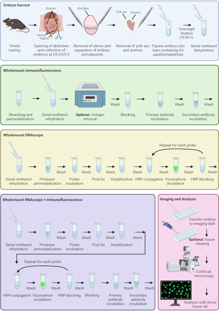
Figure 1: Immunofluorescence and RNAscope staining protocol. Schematic representing key stages of embryo harvest, immunofluorescence, RNAscope, combined immunofluorescence and RNAscope, sample imaging, and analysis. Colored boxes correspond to different protocol stages. Created in BioRender. Sparrow, D. (2026) https://BioRender.com/q6rmax8 Please click here to view a larger version of this figure.
结果
采用免疫荧光染色法对E8.5胚胎进行染色,以分析处于细胞周期G2/M期的迁移性神经嵴细胞数量。样品使用靶向PHH3的抗体染色以显示细胞周期的G2/M期,同时使用SOX10抗体标记迁移性神经嵴细胞。随后使用相应的二抗进行染色。细胞核用DAPI染色。使用Olympus SpinSR转盘共聚焦显微镜配备10倍物镜(NA = 0.4)对样品成像。图像通过Hamamatsu Orca Fusion BT相机和50 µm针孔转盘采集,并采用平铺拼接功能以Z栈形式获取,Z轴间距为1.99 µm。神经嵴细胞通过上皮-间质转化(EMT)实现脱离及后续迁移,此过程要求迁移前的神经嵴细胞处于细胞周期的S期或G2/M期20。在此,我们可观察到在迁移性神经嵴细胞群体中处于细胞周期G2/M期的细胞,其由PHH3染色(绿色)指示,而迁移性神经嵴细胞由SOX10染色(品红色)指示(图2A)。可通过定量对照组与处理组胚胎中处于G2/M期的迁移性神经嵴细胞数量,判断处理是否影响了处于G2/M期的迁移性神经嵴细胞数量,从而推断该处理是否也可能干扰通过EMT介导的神经嵴细胞脱离过程。部分胚胎在解剖后仍残留卵黄囊(图2A’,红色箭头)。由于抗PHH3抗体来源于小鼠,残留的卵黄囊对小鼠来源的二抗具有敏感性,在本样本中尤为明显,因此整个卵黄囊会因与抗小鼠抗体偶联的荧光染料而产生强烈荧光。在此极端情况下,非特异性染色可能影响PHH3信号的定量分析,因此该样本应从分析中剔除。此外,使用抗小鼠抗体时,在E8.5胚胎的心管附近常出现一条非特异性“条带”状背景信号(图2A’,红色箭头)。在对来源于小鼠的一抗信号进行定量时,应考虑该区域的干扰。
采用本方案通过免疫荧光染色E9.5胚胎,以观察血管结构和心脏前体细胞的分布。样本使用靶向ISLET1(ISL1)的抗体标记第二心区,SOX10抗体标记迁移中的神经嵴细胞,ENDOMUCIN(EMCN)抗体标记静脉和毛细血管内皮细胞,并配合相应的二抗进行染色。细胞核使用DAPI染色。通过组织透明化处理以提高成像深度。样本使用Olympus SpinSR转盘共聚焦显微镜配备10倍物镜(NA = 0.4)进行成像。在E9.5时期,可见心脏神经嵴细胞迁移并参与主动脉弓的形成(SOX10,黄色),以及第二心区前体细胞(ISL1,绿色)参与心房、心室流出道及左心室的形成21(图2B)。心脏前体细胞的异常是先天性心脏病发生的关键驱动因素22,23。利用该方法,我们能够可视化心脏前体细胞的空间分布模式及其数量。下一步可比较对照组与处理组之间心脏前体细胞分布模式的差异,以确定干预措施是否干扰了细胞迁移或导致关键细胞类型的丢失。
为了确定神经嵴细胞发育阶段与Wnt信号通路之间的关系,采用本方案通过RNAscope对E8.5胚胎进行染色,以检测处于不同迁移和分化阶段的神经嵴细胞以及Wnt信号通路的标记物。使用了分别标记神经板边界(神经嵴细胞的起源部位,Msx1)、迁移中的神经嵴细胞(Sox10)以及神经嵴细胞分化(Dlx2)的探针,并与指示Wnt信号通路的探针(Sp5)进行比较。采用TSA-vivid 520、570、650和Opal 780荧光染料对探针进行可视化。样品使用Evident FV4000显微镜成像,物镜倍数为10倍(NA=0.4),针孔大小为144 µm,像素尺寸为621 nm。通过平铺拼接功能以Z堆栈方式采集图像,Z轴间距为4.32 µm。神经板边界(Msx1,绿色)与迁移中的神经嵴细胞(Sox10,品红色)在头部占据不同的区域,部分区域存在重叠,表明细胞正从神经管开始迁移(图3A)。部分迁移中的神经嵴细胞区域与Dlx2(青色)共定位,提示部分细胞正向颅面分化方向进展(图3A)。Wnt信号通路(Sp5,黄色)存在于神经板边界区域,这一点具有重要意义,因为Wnt信号通路的调控对于神经嵴细胞的脱离和分化是必需的24,25,同时也在迁移中神经嵴细胞相邻的一个独立区域中被检测到(图3A)。
进一步染色旨在通过标记神经嵴状态和Wnt信号通路的标志物,研究E9.5时期神经嵴细胞迁移与Wnt信号通路之间的关系。用于指示神经板边界位置的探针(Msx1)以及迁移性神经嵴细胞(Sox10)被使用,并与指示 Wnt 信号通路的探针进行比较(Sp5)。使用 TSA-vivid 520、570 和 650 荧光染料对探针进行可视化。样品采用 Olympus SpinSR 转盘共聚焦显微镜,配备 10 倍物镜(NA = 0.4)进行成像。在此我们可以观察到神经板边界(Msx1,绿色),与迁移中的神经嵴细胞(Sox10 品红)(图3B). Wnt信号通路(Sp5,黄色)在胚胎背部区域明显可见,此处躯干神经嵴细胞正在发生去分化,同时在头部特定区域以及围绕1st 和 2nd 鳃弓、流出道下方以及耳囊内(图3B通过该方法比较对照组与处理组中神经嵴细胞的空间分布模式及Wnt信号通路活性,可帮助我们确定干预措施是否影响神经嵴细胞的去上皮化与迁移过程,以及任何影响是否源于Wnt信号通路的改变。
为了确定神经板边界细胞的细胞周期状态,我们采用该方案结合免疫荧光与RNAscope染色技术。使用了针对神经板边界的RNAscope探针(Msx1)。样品通过靶向PHH3和PCNA的抗体进行染色,分别用于显示细胞周期的G2/M期和S期。胚胎进一步使用相应的二抗进行染色。细胞核使用DAPI染色。样品使用Olympus SpinSR转盘共聚焦显微镜配备10倍物镜(NA = 0.4)(图4A、B),或使用Evident FV4000共聚焦显微镜配备10倍物镜(NA = 0.4)、127 µm针孔和311 nm像素尺寸进行成像(图4B’)。在此我们可以观察到处于G2/M期(PHH3,黄色)和S期(PCNA,品红色)的细胞均与神经板边界区域重叠(图4A)。利用该方法,我们可以量化神经板边界内各细胞周期阶段的细胞比例,并判断这些比例是否因处理组的不同而发生变化。值得注意的是,该胚胎中存在因使用精细镊子过度操作导致解剖损伤而形成的孔洞。这凸显了解剖过程中需格外小心以避免损伤的重要性,尤其是在E8.5时期,胚胎尤为脆弱。
将RNAscope与免疫荧光结合使用可能导致RNAscope探针的染色信号比单独进行RNAscope时更弱。当与一种荧光非常强且使用邻近荧光染料(例如Fluorescein和Cy3)的一抗结合时,可能会导致信号从较亮的通道渗漏到较暗的通道(图4B)。为避免此问题,可采用稀释度更高的高亮度抗体,选择光谱差异更大的荧光染料,或调整样本的成像参数。转盘共聚焦显微镜对胚胎成像速度很快,但由于其使用具有固定发射波长窗口的带通发射滤光片,无法动态缩小检测窗口以匹配特定荧光染料。而使用点扫描显微镜(例如Evident FV4000),操作者可精确至纳米级别调节检测窗口,因此在使用发射光谱存在轻微重叠的荧光染料时,可有效减少信号渗漏(图4B’)。
为了确定E8.5胚胎中处于细胞周期不同阶段的细胞比例,我们采用本方案分析细胞周期S期和G2/M期的细胞核比例及信号强度。样品使用靶向PHH3和PCNA的抗体进行染色,分别用于标记细胞周期的G2/M期和S期,随后使用相应的二抗进行染色。细胞核使用DAPI染色。采用Olympus SpinSR转盘共聚焦显微镜配备10x物镜(NA = 0.4)对样品进行成像。使用Zeiss Arivis Pro软件识别所有细胞核、PHH3阳性细胞核、PCNA阳性细胞核以及双阳性细胞核(图5A)。通过该方法,我们能够比较处于细胞周期G2/M期(PHH3+)和S期(PCNA+)的细胞比例(图5B),以及每个单独细胞核中PHH3或PCNA染色的强度(图5C)。结果显示,心脏区域PCNA+细胞核的比例略高于头部区域和整个胚胎(图5B)。此外,头部区域PHH3+和双染细胞核的比例高于心脏区域和整个胚胎(图5B)。各区域之间PHH3或PCNA染色强度无明显差异(图5C)。上述数据来源于一个代表性胚胎(n = 1),旨在展示分析流程;未进行推论性统计分析。综上,该方法使我们能够在心脏和颅面发育关键阶段,确定细胞周期传播的模式。该方法将有助于判断我们的处理是否影响胚胎不同区域的细胞周期进程。
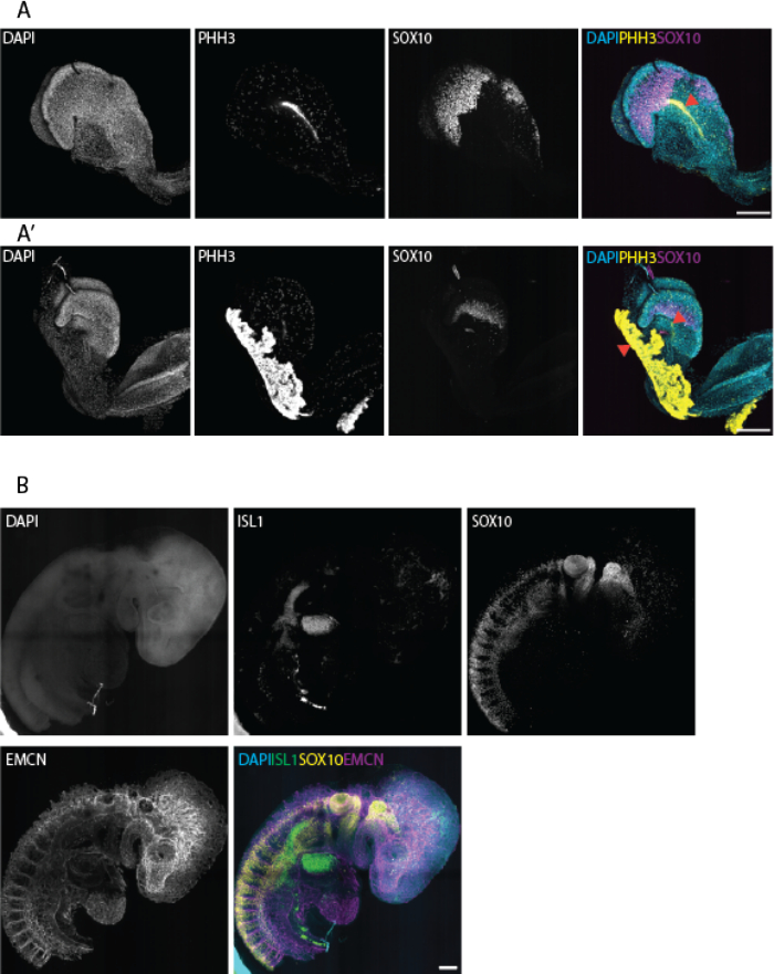
图2:E8.5 和 E9.5 胚胎中蛋白质的免疫荧光染色。(A, A’)对 E8.5 小鼠胚胎进行免疫荧光染色,以 PHH3 标记细胞周期 G2/M 期的细胞,SOX10 标记迁移中的神经嵴细胞,DAPI 标记细胞核。N = 1 次实验中的 11 个胚胎。(B)对 E9.5 胚胎进行 ISL1 染色以标记第二心区前体细胞,SOX10 染色以标记迁移中的神经嵴细胞,EMCN 染色以标记毛细血管和静脉血管,以及 DAPI 染色以标记细胞核。红色箭头指示卵黄囊中的非特异性染色,以及 胚胎内抗小鼠二抗产生的非特异性染色(n = 1 次实验中的 15 个胚胎)。比例尺 = 200 µm。DAPI:4′,6-二脒基-2-苯基吲哚;PHH3:磷酸化组蛋白 H3;EMCN:内黏蛋白。请点击此处查看该图的放大版本。
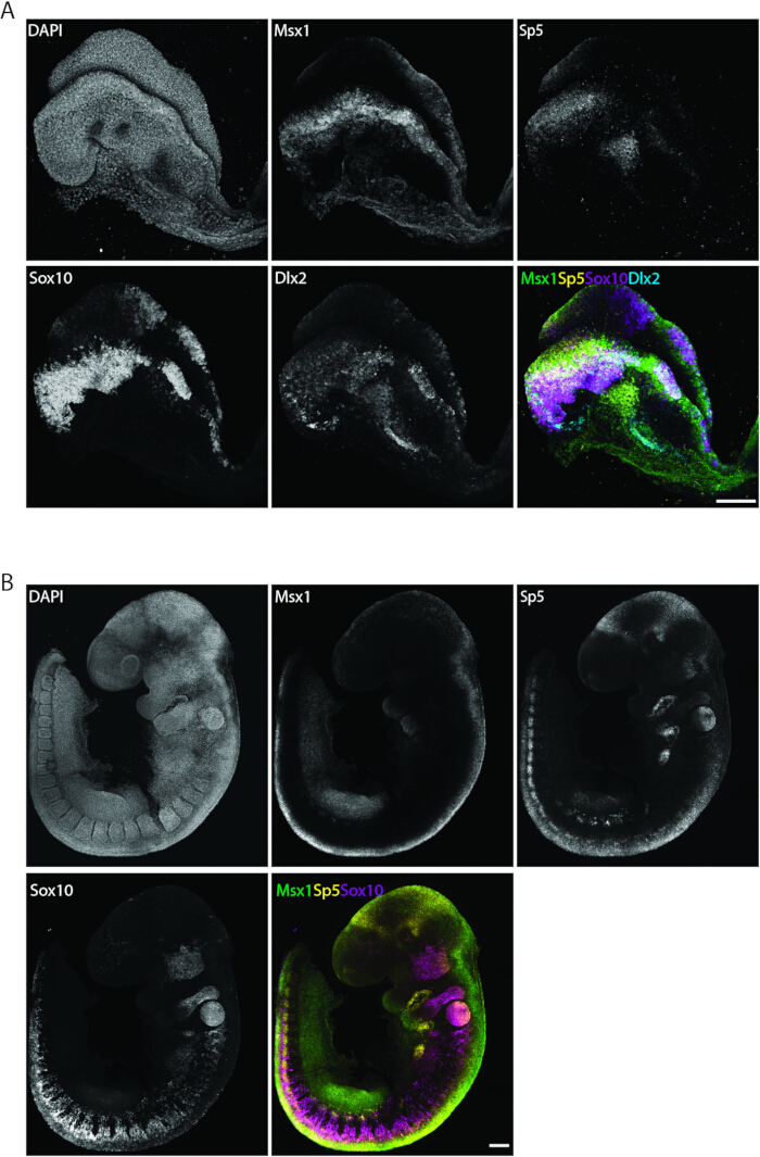
图3:通过RNAscope对E8.5和E9.5胚胎中的转录本进行染色。 (A) E8.5 胚胎经 RNAscope 染色,探针靶向 Msx1 可视化神经板边界, Sox10 以观察迁移中的神经嵴 Dlx2 以观察神经嵴的分化过程,以及 Sp5 用于Wnt信号通路。n = 13个胚胎,来自1次实验。(BE9.5 胚胎经 RNAscope 染色,探针靶向 Msx1 可视化神经板边界, Sox10 以观察迁移中的神经嵴, Sp5 以可视化 Wnt 信号通路。n = 1 次实验中的 4 个胚胎。比例尺 = 200 µm. 请点击此处以查看此图的放大版本。
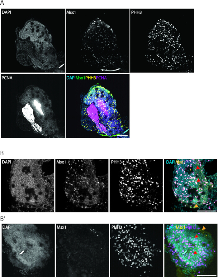
图4E8.5 胚胎中联合免疫荧光染色与 RNAscope 检测 (A,B,B’) E8.5 胚胎经 RNAscope 染色,探针靶向 Msx1 通过免疫荧光标记PCNA以显示细胞周期S期的细胞,以及PHH3抗体以显示细胞周期G2/M期的细胞,从而可视化神经板边界。橙色箭头指示特定 Msx1 染色,红色箭头指示荧光串色,(B),或特异性PHH3染色且无渗漏至Msx1通道(B')。N = 1 次实验中的 2 个胚胎。比例尺 = 200 µm. 请点击此处以查看此图的放大版本。
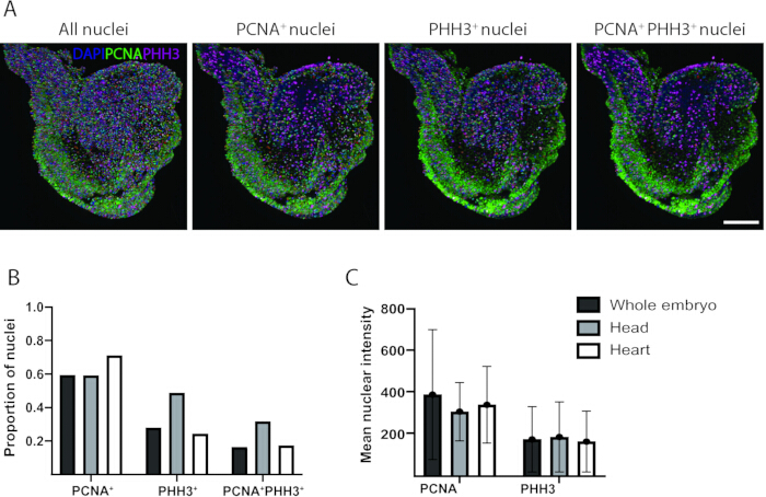
图5使用 Arivis Pro 分析 E8.5 胚胎的细胞周期阶段 (A) E8.5小鼠胚胎经免疫荧光染色,使用PCNA标记细胞周期S期细胞(绿色),PHH3标记细胞周期G2/M期细胞(洋红色),DAPI标记细胞核(蓝色)。检测到的三维对象(多色球体)通过蔡司Arivis Pro中的4D观察器进行叠加与可视化。B) 该图展示了PCNA的比例+PHH3+,以及单个胚胎全身、头部和心脏中的双阳性细胞核。C) 该图展示了单个胚胎整体、头部和心脏中每个细胞核的 PCNA 和 PHH3 染色平均强度。圆圈代表平均值;误差线代表单个样本内所有细胞核的标准差。图表使用 GraphPad Prism 制作。比例尺 = 200 µm对 n = 1 个胚胎进行了定量分析。未进行推断性统计分析。误差线表示单个细胞核之间的标准差。3D:三维;DAPI:4′,6-二脒基-2-苯基吲哚 请点击此处以查看此图的放大版本。
讨论
本文介绍了一种优化的方法,用于在E8.5和E9.5全胚胎标本中空间分析基因和蛋白质的表达。与传统的RNA 原位 杂交和组织切片免疫荧光方法相比,该方法具有更高的空间分辨率和多重检测能力。本方案在现有最新方案的基础上,进一步用于研究小鼠胚胎的发育通路。最近一项研究利用RNAscope与免疫荧光染色技术检测胚胎中的Wnt信号通路,但其染色对象为组织切片而非全胚胎标本26。另一项近期研究对E8.5至E10.5阶段的全胚胎小鼠标本进行了全胚胎RNAscope和免疫荧光染色27,但作者未将两种染色技术结合使用,也未使用C4探针和Opal 780荧光染料实现第四通道的RNAscope染色。联合使用免疫荧光与RNAscope技术此前已在E3.5全胚胎中有所报道,其中RNAscope在完成免疫荧光流程后进行28。尽管我们尚未在较晚期胚胎中尝试该确切方案,但在E8.5胚胎中,若将RNAscope染色夹在免疫荧光的一抗与二抗孵育之间,则抗体染色效果较差。这可能是由于对较大胚胎进行RNAscope时需要蛋白酶孵育步骤,而E3.5胚胎的研究中无需此步骤。蛋白酶孵育可能影响已结合抗体的完整性,因此在该系统中调换RNAscope与免疫荧光的顺序可能不可行。另一项近期在肌纤维中的研究通过在免疫荧光染色前进行RNAscope实现了两种方案的结合29。与本方案类似,该研究也是先进行RNAscope再进行免疫荧光;然而,该方法未在全胚胎小鼠标本中验证其流程,也未通过C4探针与Opal 780荧光染料实现额外RNAscope通道的染色。
利用多重标记技术对整体胚胎进行染色,在发育生物学中具有广泛的应用价值,可用于定位关键的转录本和蛋白质,标记不同发育阶段胚胎中的前体细胞类型或发育相关信号通路。我们已成功应用这些技术绘制了心脏前体细胞的分布图谱(图 2B)、不同迁移和分化阶段的神经嵴细胞(图 3)、Wnt 信号通路(图 3)以及细胞周期阶段(图 2,图 4,图 5)。通过调整所使用的探针和抗体,该技术可用于检测任何感兴趣的细胞类型或信号分子,只要这些分子在该发育阶段的胚胎中存在即可。尽管本方案主要聚焦于 E8.5 和 E9.5 阶段的胚胎,但通过优化组织通透化处理、孵育时间及组织透明化步骤,也可能实现对更早期或更晚期胚胎的染色。
然而,这种在整体胚胎中同时检测蛋白质和转录本表达的能力增强也带来了新的挑战。首先,与切片样本上的免疫荧光和RNAscope检测相比,整体样本的分析更为耗时,后者通常可在1–2天内完成,而整体样本则需要多日。此外,使用整体样本需要仔细考虑显微成像参数,以确保足够的成像深度和分辨率。需要配备能够穿透尽可能厚的样本进行成像的显微镜,其成像深度可达 700 µm 厚组织样本需要对较大的胚胎使用组织透明化技术,否则可能遗漏样本深层的结构。此外,由于样本较厚,使用宽场显微镜成像会导致大量来自焦平面外的光线被采集,从而影响图像质量;而共聚焦显微镜因其能够消除焦平面外信号的能力,可实现对样本的逐层成像并排除非焦平面信号,因此更为适用。其中,转盘式共聚焦显微镜通常可实现更快的图像采集速度,但在荧光信号检测的精细控制方面相较于点扫描共聚焦显微镜有所折衷。胚胎的尺寸也可能带来挑战,因为许多显微镜的视场不足以在无需拼接扫描的情况下完整成像整个胚胎,这可能导致图像中出现拼接伪影(例如, 图2B)。多重检测样本还可能导致通道间串扰(例如, 图 4B), 可通过选择点扫描共聚焦显微镜来减轻这一问题,该显微镜能够缩小检测窗口,适用于发射光谱略有重叠的荧光染料。使用Opal 780荧光染料有助于在单个样本中进一步实现多靶标多重检测;但需要具备近红外成像能力的显微镜才能检测该系统,而大多数光学显微镜不具备此项功能。
成像样品的封片也需要仔细考虑。如果让样品自由漂浮(例如在多孔板腔室载玻片中成像),样品在成像时并不总处于完全相同的角度,这可能导致染色强度的差异,具体取决于胚胎的哪些部分最接近相机/探测器,从而在后续的强度分析中带来挑战。使用多孔腔室载玻片的另一个问题是,孔的边缘可能位于成像视野内,从而在图像中产生伪影。将胚胎固定在凹面载玻片中虽有助于保持方向一致,但容易造成胚胎损伤和/或压缩,使结构的体积分析变得困难。
在执行本方案时,需考虑若干因素。进行免疫荧光染色时,在抗原修复过程中需特别注意避免胚胎解离,尤其是在分析较早期胚胎时。为避免此问题,可尝试采用其他抗原修复方法,例如使用Tris/EDTA等替代缓冲液,或采用蛋白酶消化法进行抗原修复。对于较小或较大的胚胎,可能需要优化抗体孵育时间。选择一抗时需谨慎,因为许多抗体是在小鼠体内产生的,而使用抗小鼠二抗可能会与残留的卵黄囊结合并产生强荧光信号。该现象在使用AlexaFluor 488标记的抗小鼠二抗(图2)和AlexaFluor 647标记的抗小鼠二抗(图4)时可见。本实验室尚未测试其他荧光染料,但不同荧光染料的荧光强度可能存在差异,需进一步优化。在使用抗兔(图2、图4、图5)或抗大鼠抗体(图2B)的荧光通道中未观察到此类非特异性信号,因此建议在可行的情况下优先选用非小鼠来源的一抗。
对于RNAscope实验,优化蛋白酶孵育步骤至关重要,因为孵育时间过短会导致探针渗透不足,而时间过长则可能导致样本完全解离。在优化蛋白酶孵育时间时,建议每次仅调整1分钟。最佳实践还包括使用适当的对照,以确定探针或抗体是否有效。阴性对照可采用相同发育阶段的胚胎,同时进行染色但不加探针或不加一抗,或分别使用IgG同型对照或阴性对照探针,用于免疫荧光或RNAscope,以确认所观察到的染色信号是真实的。此外,使用已知表达目标基因或转录本的大小相当的组织作为阳性对照,也有助于判断染色是否成功。
总体而言,本方案是一种稳定且经过优化的方法,可用于在E8.5和E9.5期小鼠胚胎整体标本中可视化蛋白和转录本的表达,在研究正常胚胎发育及疾病中的细胞与分子机制方面具有广阔的应用前景。
披露
作者声明无竞争性财务利益。
致谢
作者感谢牛津大学人类遗传学中心细胞成像核心设施团队为本手稿中涉及的显微镜技术和图像分析提供的技术支持。作者感谢牛津大学生物医学服务中心工作人员在动物饲养以及定时交配以获取胚胎方面给予的支持。
本研究的资助来自英国心脏基金会高级研究员项目 FS/SBSRF/22/31022(DBS)、Additional Ventures 单心室基金(DBS)、牛津大学 John Fell 基金 0016065(VSR)以及牛津大学医学科学内部基金 0016707(VSR)。
材料
| 姓名 | 公司 | 目录编号 | 评论 |
|---|---|---|---|
| 塑料器皿/玻璃器皿 | |||
| 3 ml 胎牛血清移液管,低密度聚乙烯(LDPE)带刻度 | Wheaton | 711116 | |
| Eppendorf 安全锁 1.5 ml 微量离心管 | Eppendorf | 0030 120.086 | |
| Ibidi µ-slide 18 孔板 | Ibidi | 81817 | #1.5H 玻璃盖玻片,未处理 |
| Menzel X1000 盖玻片 22×50 mm #1.5 (0.16–0.19 mm) | Thermo Scientific | 17284904 | |
| 带凹槽的载玻片 | Marienfeld Superior | 1320000 | |
| 安全密封微量离心管 2 ml | Sarstedt | 72.695.500 | 2 ml “Eppendorf”管,圆底 |
| 溶液/缓冲液 | |||
| 1× 抗体稀释/封闭液 | Akoya Biosciences | ARD1001EA | |
| Ambion™ RnaseZap™ RNase 去污染溶液 | Ambion | 9780.9782 | |
| 柠檬酸盐抗原修复缓冲液 | Vector labs | H-3300 | 标记为抗原修复液, 柠檬酸为基础 |
| 二甲基亚砜(DMSO) | Merck (Sigma-Aldrich) | D8418 | |
| Hanks' 平衡盐溶液 10× | Merck (Sigma-Aldrich) | H4641 | |
| 过氧化氢溶液 | Merck (Sigma-Aldrich) | H1009 | 30% (w/w) 水溶液 |
| 甲醇 | Merck (Sigma-Aldrich) | 32213-2.5L-M | |
| 正常驴血清 | Abcam | Ab7475 | 100% 储存浓度, 最终浓度 10% |
| 多聚甲醛(PFA)粉末 | Merck (Sigma-Aldrich) | 158127-500g | 用水稀释至 4%。在通风橱中配制。加热搅拌,并加入少量 NaOH 以促进溶解。pH 7.2–7.6 |
| 磷酸盐缓冲液(PBS) | Merck (Sigma-Aldrich) | P4417 | 每 200 ml 蒸馏水溶解 1 片 |
| RNAscope 4-Plex 辅助试剂盒(用于多重荧光检测试剂盒 v2) | ACD (Bio-Techne) | 323120 | 包含 HRP-C4 和 HRP 封闭剂 |
| RNAscope™ 多重荧光检测试剂盒 v2 | ACD (Bio-Techne) | 323110 | 包含蛋白酶 Plus、蛋白酶 III、 蛋白酶 IV、过氧化氢、TSA 缓冲液、 Amp1/2/3、Hrp-C1/2/3、HRP-封闭剂和 DAPI |
| 盐水-柠檬酸钠(SSC)缓冲液 20× 溶液 | Fisher Bioreagents | BP-1325-1 | 用蒸馏水稀释至 0.2× |
| 组织透明试剂 Cubic-R+(M) [用于动物] | Tokyo Chemical Industry | T3741 | |
| Triton™ X-100 | Merck (Sigma-Aldrich) | X100 | |
| Tween® 20 | Merck (Sigma-Aldrich) | P7949 | |
| Ultrapure™ 0.5 M EDTA,pH 8 | Invitrogen | 15575020 | |
| 一抗 | |||
| 内粘蛋白抗体(V.7C7) | Santa Cruz | SC-65495 | 使用 1:50 稀释。 |
| 胰岛素瘤相关抗原 1 和 2 抗体 | 发育研究杂交瘤库 | 34.4DS-5 | 用甘油稀释 50%。使用 1:50 稀释。 |
| PCNA(PC10)小鼠单克隆抗体 | Cell Signaling Technology | 2586S | 使用 1:500 稀释 |
| 磷酸化组蛋白 H3(Ser10)(6G3)小鼠单克隆抗体 | Cell Signaling Technology | 9706S | 使用 1:500 稀释 |
| 磷酸化组蛋白 H3(Ser10)(D7N8E)XP® 兔单克隆抗体 | Cell Signaling Technology | 53348S | 使用 1:500 稀释 |
| Sox10(E6B6I)XP® 兔单克隆抗体 | Cell Signaling Technology | 69661S | 使用 1:500 稀释 |
| 二抗/核染料 | |||
| AlexaFluor® 488 标记的 Affinipure® 驴抗小鼠 IgG(H+L) | Jackson Immunoresearch | 715-545-151 | 使用 1:500 稀释 |
| AlexaFluor® 647 标记的 Affinipure® 驴抗大鼠 IgG(H+L) | Jackson Immunoresearch | 712-605-153 | 使用 1:500 稀释 |
| AlexaFluor® 647 标记的 Affinipure® F(ab')2 片段驴抗小鼠 IgG(H+L) | Jackson Immunoresearch | 715-606-150 | 使用 1:500 稀释 |
| Cy™3 标记的 Affinipure® 驴抗兔 IgG(H+L) | Jackson Immunoresearch | 711-165-152 | 使用 1:500 稀释 |
| DAPI | Merck (Sigma-Aldrich) | D9542 | 使用浓度为 1 µg/ml |
| RNAscope 探针 | |||
| RNAscope® 探针 - Mm Sp5-C4 | ACD (Bio-Techne) | 405681-C4 | C4 探针 |
| RNAscope® 探针 - Mm-Dlx2-C3 | ACD (Bio-Techne) | 555951-C3 | C3 探针 |
| RNAscope® 探针 - Mm-Msx1 | ACD (Bio-Techne) | 421841 | C1 探针 |
| RNAscope® 探针 - Mm-Sox10-C2 | ACD (Bio-Techne) | 435931-C2 | C2 探针 |
| RNAscope 荧光染料 | |||
| Opal 780 试剂包 | Akoya Biosciences | FP1501001KT | 包含 Opal 780 试剂、Opal TSA-DIG、 DMSO |
| TSA-vivid™ 荧光染料 520 | ACD (Bio-Techne) | 323271 | 现为 ClariTSA™ 荧光染料 520 |
| TSA-vivid™ 荧光染料 570 | ACD (Bio-Techne) | 323272 | 现为 ClariTSA™ 荧光染料 570 |
| TSA-vivid™ 荧光染料 650 | ACD (Bio-Techne) | 323273 | 现为 ClariTSA™ 荧光染料 650 |
| 仪器/软件 | |||
| Fluoview FV4000 激光扫描 显微镜 | Evident | fv4000 | 激发激光:405/488/561/640/730 nm。 检测波长(图 3):430–470、500–540、570–620、 650–710、750–850 nm。检测波长(图 4):430–470、 500–531、570–620 nm。 |
| Graphpad Prism 10 | Graphpad | v10.6.1 | |
| 加热金属块 | Grant | QBT1 | |
| Hybrigene 杂交炉 | Techne (Bibby Scientific) | FHB4DD | |
| Ixplore IX83 SpinSR 超分辨率显微镜系统 | Olympus | ixplore-ix83-spinsr | 激发激光:405/488/561/640 nm。 发射滤光片:447/60、525/50、617/73、685/40。 |
| Zeiss Arivis Pro | Carl Zeiss Microscopy GmbH | v. 4.5(原为 Arivis Vision 4D) | |
| Zeiss Arivis SIS 转换器 | Carl Zeiss Microscopy GmbH | v. 4.3.0 |
参考文献
- Bruter AV, Varlamova EA, Okulova YD, Tatarskiy VV, Silaeva YY, Filatov MA. Genetically modified mice as a tool for the study of human diseases. Mol Biol Rep. 2024;51(1):135.
- Rashbrook VS, Brash JT, Ruhrberg C. Cre toxicity in mouse models of cardiovascular physiology and disease. Nat Cardiovasc Res. 2022;1:806–16.
- Breschi A, Gingeras TR, Guigo R. Comparative transcriptomics in human and mouse. Nat Rev Genet. 2017;18(7):425–40.
- Mole MA, Weberling A, Zernicka-Goetz M. Comparative analysis of human and mouse development: From zygote to pre-gastrulation. Curr Top Dev Biol. 2020;136:113–38.
- Krishnan A, Samtani R, Dhanantwari P, Lee E, Yamada S, Shiota K, et al. A detailed comparison of mouse and human cardiac development. Pediatr Res. 2014;76(6):500–7.
- Anderson RH, Bamforth SD. Morphogenesis of the Mammalian Aortic Arch Arteries. Front Cell Dev Biol. 2022;10:892900.
- Wessels A, Sedmera D. Developmental anatomy of the heart: a tale of mice and man. Physiol Genomics. 2003;15(3):165–76.
- Gall JG, Pardue ML. Formation and detection of RNA-DNA hybrid molecules in cytological preparations. Proc Natl Acad Sci U S A. 1969;63(2):378–83.
- John HA, Birnstiel ML, Jones KW. RNA-DNA hybrids at the cytological level. Nature. 1969;223(5206):582–7.
- Buongiorno-Nardelli M, Amaldi F. Autoradiographic detection of molecular hybrids between RNA and DNA in tissue sections. Nature. 1970;225(5236):946–8.
- Dakou E, Vanbekbergen N, Corradi S, Kemp CR, Willems E, Leyns L. Whole-mount in situ hybridization (WISH) optimized for gene expression analysis in mouse embryos and embryoid bodies. Methods Mol Biol. 2014;1211:27–40.
- Anderson R. Multiplex fluorescence in situ hybridization (M-FISH). Methods Mol Biol. 2010;659:83–97.
- Kearney L. Multiplex-FISH (M-FISH): technique, developments and applications. Cytogenet Genome Res. 2006;114(3-4):189–98.
- Burnett R, Guichard Y, Barale E. Immunohistochemistry for light microscopy in safety evaluation of therapeutic agents: an overview. Toxicology. 1997;119(1):83–93.
- Coons AH, Creech HJ, Jones RN. Immunological properties of an antibody containing a fluorescent group. P Soc Exp Biol Med. 1941;47(2):200–2.
- Bardot E, Tzavaras N, Benson DL, Dubois NC. Quantitative Whole-mount Immunofluorescence Analysis of Cardiac Progenitor Populations in Mouse Embryos. J Vis Exp. 2017(128).
- Wang F, Flanagan J, Su N, Wang LC, Bui S, Nielson A, et al. RNAscope: a novel in situ RNA analysis platform for formalin-fixed, paraffin-embedded tissues. J Mol Diagn. 2012;14(1):22–9.
- Erben L, Buonanno A. Detection and Quantification of Multiple RNA Sequences Using Emerging Ultrasensitive Fluorescent In Situ Hybridization Techniques. Curr Protoc Neurosci. 2019;87(1):e63.
- De Bono C, Lescroart F, Zaffran S. How to Study Gene Expression and Gain of Function of Hoxb1 in Mouse Heart Development. Methods Mol Biol. 2025;2889:121–37.
- Zhao R, Moore EL, Gogol MM, Unruh JR, Yu Z, Scott AR, et al. Identification and characterization of intermediate states in mammalian neural crest cell epithelial to mesenchymal transition and delamination. Elife. 2024;13.
- Guijarro C, Kelly RG. On the involvement of the second heart field in congenital heart defects. C R Biol. 2024;347:9–18.
- Bradshaw L, Chaudhry B, Hildreth V, Webb S, Henderson DJ. Dual role for neural crest cells during outflow tract septation in the neural crest-deficient mutant Splotch(2H). J Anat. 2009;214(2):245–57.
- Zawada D, Kornherr J, Meier AB, Santamaria G, Dorn T, Nowak-Imialek M, et al. Retinoic acid signaling modulation guides in vitro specification of human heart field-specific progenitor pools. Nat Commun. 2023;14(1):1722.
- Rabadan MA, Herrera A, Fanlo L, Usieto S, Carmona-Fontaine C, Barriga EH, et al. Delamination of neural crest cells requires transient and reversible Wnt inhibition mediated by Dact1/2. Development. 2016;143(12):2194–205.
- Bhattacharya D, Rothstein M, Azambuja AP, Simoes-Costa M. Control of neural crest multipotency by Wnt signaling and the Lin28/let-7 axis. Elife. 2018;7.
- Kishimoto K, Furukawa KT, Luz-Madrigal A, Yamaoka A, Matsuoka C, Habu M, et al. Bidirectional Wnt signaling between endoderm and mesoderm confers tracheal identity in mouse and human cells. Nat Commun. 2020;11(1):4159.
- De Bono C, Liu Y, Ferrena A, Valentine A, Zheng D, Morrow BE. Single-cell transcriptomics uncovers a non-autonomous Tbx1-dependent genetic program controlling cardiac neural crest cell development. Nat Commun. 2023;14(1):1551.
- Hazra R, Spector DL. Simultaneous visualization of RNA transcripts and proteins in whole-mount mouse preimplantation embryos using single-molecule fluorescence in situ hybridization and immunofluorescence microscopy. Front Cell Dev Biol. 2022;10:986261.
- Kann AP, Krauss RS. Multiplexed RNAscope and immunofluorescence on whole-mount skeletal myofibers and their associated stem cells. Development. 2019;146(20).
重印与许可
本文已发表
视频即将推出