This review examines perturbation- and backpropagation-based explainable artificial intelligence methods for medical imaging, comparing their principles, strengths, limitations, and clinical applications, and highlighting current challenges and future directions to improve interpretability and trust in AI-assisted healthcare.
Übersichtsartikel
Towards Explainable Artificial Intelligence in Medical Imaging: A Review of Perturbation and Backpropagation-Based Methods
In diesem Artikel
Zusammenfassung
Zusammenfassung
Machine and deep learning algorithms have been proven their efficiency in the medical domain. This is particularly noticeable in medical imaging, where these algorithms have demonstrated exceptional capabilities, often surpassing human experts in detecting diseases, segmenting anatomical structures, and in aiding diagnosis. However, despite their high performance, the non-transparency of these models has raised concerns about trust and explainability, especially in critical domains, such as healthcare. Explainable AI (XAI) has emerged as a promising field that, aims to make the decision-making processes of AI systems more interpretable and understandable to humans. By offering clear, human-understandable justifications, XAI enhances clinicians’ trust in AI-assisted decisions, and supports the safe integration of these technologies into clinical workflows. This paper focuses on perturbation-based and backpropagation-based explainability methods that are widely adopted for convolutional neural networks in medical imaging. We intend to provide deeper insight into the relevance of XAI methods in medical imaging. We propose a structured taxonomy that categorizes these methods into perturbation and backpropagation-based approaches. For each category, we highlight their respective strengths, limitations, and areas of applicability. Furthermore, we discuss the key challenges hindering the adoption of XAI and identify promising research directions to bridge the gap between high-performance AI models and their responsible deployment in real-world healthcare environments.
Einleitung
Advances in computational power have been a critical driver of artificial intelligence (AI) over the past decades1. As a result, AI has experienced unprecedented progress, transforming diverse domains by automating complex tasks and enabling systems to emulate aspects of human intelligence. These advances have led to the emergence of several major research areas, including deep learning (DL), computer vision (CV), natural language processing (NLP), and large language models (LLMs)2. Among these, deep learning and computer vision have demonstrated remarkable success in medical imaging3, where they support a wide range of tasks such as image enhancement, classification, segmentation, registration, and disease detection. By exploiting information acquired from imaging modalities such as X-ray, computed tomography (CT), magnetic resonance imaging (MRI), and ultrasound, AI-based systems have achieved outstanding performance in detecting abnormalities4, diagnosing diseases5, and assisting clinicians in medical decision-making6. Convolutional neural networks (CNNs) have enabled automated image analysis with diagnostic accuracy that, in some applications, rivals or even surpasses human experts.
Despite these achievements, the rapid increase in predictive performance has been accompanied by a corresponding increase in model complexity. Most state-of-the-art AI models, particularly deep neural networks, operate as blackbox systems whose internal decision-making processes remain difficult to interpret7. This lack of transparency raises important concerns regarding trust, accountability, fairness, and patient safety, especially in high-stakes domains such as healthcare, where clinical decisions directly affect patient outcomes. Consequently, although AI has demonstrated exceptional potential in medical imaging, its adoption in routine clinical practice remains limited, as clinicians often require clear justification before relying on AI-assisted diagnoses. This has led to a fundamental trade-off between predictive accuracy and interpretability: while inherently interpretable models, such as decision trees and linear models, provide greater transparency at the expense of predictive performance, more complex architectures, such as deep neural networks, generally achieve higher accuracy but offer limited insight into their decision-making process (Figure 1).
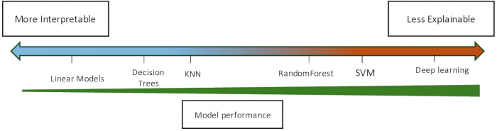
Figure 1. Model performance versus explainability. Abbreviations: kNN = k-nearest neighbors; SVM = Support Vector Machine. Please click here to view a larger version of this figure.
These challenges naturally raise two fundamental questions: How can high predictive performance be maintained while improving model transparency, and how can clinicians understand and trust AI-assisted decisions without compromising diagnostic accuracy? Addressing these questions has led to the emergence of explainable Artificial Intelligence (XAI)8, a research field dedicated to making AI systems more transparent and understandable to human users. In medical imaging, XAI enables clinicians to understand the rationale behind model predictions, validate diagnostic outcomes, and identify image regions that contribute to automated decisions, thereby strengthening confidence in AI-assisted diagnosis while supporting ethical and accountable clinical practice9. Furthermore, XAI can reveal potential biases in AI-driven pathological assessments10, allowing medical experts to identify features that may inadvertently influence diagnostic decisions (Figure 2).
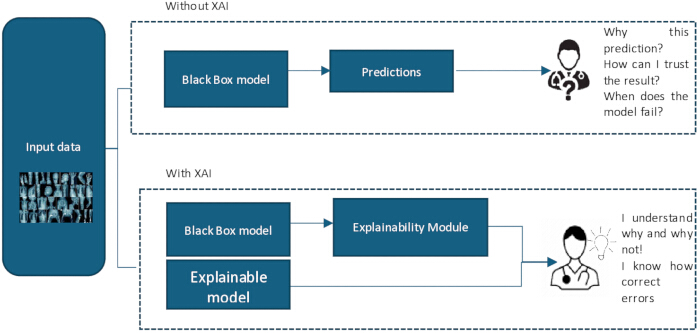
Figure 2. Conceptual depiction of the interaction between AI models and end-users with/without explainable AI. Abbreviation: XAI = explainable AI. Please click here to view a larger version of this figure.
However, explainability in medical imaging is not solely a technological challenge. Its successful adoption also depends on medical, ethical, legal, and regulatory considerations. From a clinical perspective, explanations must be meaningful and compatible with existing diagnostic workflows. From a legal and ethical standpoint, AI systems must comply with requirements related to transparency, accountability, patient privacy, and fairness. In this review, however, we focus exclusively on the technological perspective of explainable artificial intelligence in medical imaging.
Our objective is to provide a focused review of perturbation-based and backpropagation-based explainability methods and to analyze their role in improving the interpretability, trustworthiness, and clinical applicability of AI-driven diagnostic systems. Several recent surveys have reviewed the broad landscape of explainable artificial intelligence in medical imaging, including comprehensive surveys of deep learning visualization techniques11 and recent systematic reviews covering XAI techniques, clinical applications, and associated challenges12. In contrast, this review adopts a focused perspective by examining perturbation-based and backpropagation-based explainability methods within a unified taxonomy. Beyond describing these methods, the review comparatively analyzes their theoretical foundations, computational trade-offs, robustness, faithfulness, quantitative evaluation strategies, and clinical applicability, providing a structured synthesis intended to support researchers and practitioners in selecting appropriate explainability techniques for medical imaging applications.
This review focuses on perturbation- and backpropagation-based post hoc explainability methods developed primarily for two-dimensional convolutional neural networks (CNNs) and widely applied in medical image analysis. Although these techniques remain among the most established and widely adopted XAI approaches in clinical imaging, they do not encompass the full scope of explainable artificial intelligence. Recent developments, including attention-based attribution methods for Vision Transformers (ViTs)13, concept-based explanations (e.g., TCAV)14, prototype-based learning15, counterfactual explanations, and other intrinsically interpretable approaches, are beyond the scope of this review because they rely on fundamentally different explanation mechanisms and evaluation paradigms. Likewise, although the reviewed methods have been extensively applied to volumetric imaging modalities such as CT and MRI, their presentation in this review primarily follows their formulation for two-dimensional CNN architectures, which constitute the methodological foundation of many subsequent medical imaging applications.
Überprüfung und Perspektive
Literature selection strategy
This review provides a focused analysis of perturbation-based and backpropagation-based explainability methods for medical imaging. The literature was selected to cover the seminal methods, major methodological developments, and representative applications in medical imaging.
Relevant publications were identified through searches of major scientific databases, including IEEE Xplore, PubMed, Scopus, and Web of Science, using combinations of keywords such as Explainable Artificial Intelligence, XAI, Medical Imaging, Saliency Maps, Grad-CAM, Integrated Gradients, LIME, SHAP, Layer-wise Relevance Propagation, and Occlusion Sensitivity. Additional relevant studies were identified from the reference lists of highly cited publications.
The selection was performed by the authors based on relevance to the scope (perturbation-based and backpropagation-based methods for medical imaging) and methodological contribution. Priority was given to peer-reviewed journal articles and conference papers that introduce influential explainability methods or report significant applications in medical imaging. Emphasis was placed on studies that have shaped the development of perturbation-based and backpropagation-based explainability techniques. Because the objective of this work is to provide a methodological synthesis rather than a quantitative systematic review or meta-analysis, no formal PRISMA screening procedure or study quality assessment was performed.
Taxonomies of explainable AI methods
Numerous methods have been proposed in response to the increasing demand to understand the reasons behind ML algorithms' decisions, each developed to address explainability issues (when, how, …). Several taxonomies have been proposed to organize XAI methods according to their underlying principles, model dependence, and explanation mechanisms16. Recent reviews have further organized explainability approaches for medical imaging into categories such as perturbation-based, gradient-based, decomposition-based, attention-based, and transformer-based methods11. Although these taxonomies offer a useful foundation for understanding and selecting XAI techniques, it is important to note that there is no single, universally accepted taxonomy. The distinctions between these categories are ambiguous, and the classification may vary depending on the use case. In this section, we briefly present the most widely used taxonomies; a comprehensive analysis can be found in these studies10,17.
Model-specific vs model-agnostic
Model-specific methods have been developed for specific machine learning architectures. They used the model's internal structure and parameters to explain. Therefore, they offer deeper insight and more precise explanations. However, they lack generalizability because their explanations cannot be extended to other types of models, and they can be complex to implement and difficult to understand because of their reliance on the model’s architecture.
Global model vs local model
Global explainable methods aim to explain the overall behavior of the entire model. They described how the model made final decisions across all the possible input data. Global methods explain the general trends and patterns a model learns by simplifying its underlying logic. By contrast, local methods concentrate on a particular input instance. These methods were designed to explain why the model makes a particular decision in that case. This makes them useful for anomaly detection and justifies individual decisions. However, they can be computationally expensive and may fail to detect the systematic biases present in the model. Global methods, however, require a high-level understanding of the model and may oversimplify its overall behavior, omitting nuances in complex datasets.
Pre-model vs in-model vs post-model
The explainability process can occur before the model is built. During data preparation, we discuss pre-model methods to clarify the input data and make the modeling process more transparent. This category of XAI models ensures that the input variables are meaningful and understandable, thereby improving explainability without relying on the model’s architecture. In-model methods focus on integrating explainability directly into a model’s structure during construction. Other methods, implemented after building the model, are called post-model methods. They provided explanations for the behavior of an already-trained model without altering its structure.
Surrogate vs visualization
Surrogate methods involve creating a simpler, interpretable model to analyze a more complex one. The surrogate model can approximate the blackbox model’s behavior, making it easier to understand its decision pattern. It uses the same input data as the blackbox model; however, rather than being trained on the true labels, it is trained on the complex model's predictions. Decision trees and linear regression are examples of surrogate models. The main disadvantage of these methods is that the surrogate model can oversimplify or potentially miss subtle patterns. Visual methods create visual representations, such as plots, charts, or heatmaps, to provide insights into the model’s inner workings, making it easier to identify relevant features that contribute to the model’s decision.
Intrinsic vs post-hoc
Intrinsic methods18 refer to models that are inherently explainable through design. Their architecture is transparent and understandable and does not require additional methods or tools for explanation. Typical examples include linear models and decision trees19,20. However, post hoc methods apply explainability techniques after predictions are made. They are used for blackbox models where intrinsic interpretability is lacking. They can be harder to implement and understand than intrinsic methods; however, they are more flexible. Figure 3 shows a flow chart of the different taxonomies.
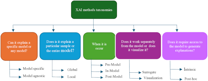
Figure 3. Classification criteria for explainable AI methods. Abbreviation: XAI = explainable AI. Please click here to view a larger version of this figure.
XAI methods in medical imaging
In medical imaging, explainability methods are generally divided into visual (saliency-based) and non-visual methods. While common saliency-based methods focus on generating visual representations to highlight medical image regions that contribute to the model’s decision-making21, non-visual methods aim to provide explanations for textual22 and tabular data, as well as statistical analyses. Visual methods calculate the attribution of each input feature (pixel or region) to the model output. These attributions are visualized as attribution maps, which are often represented as heatmaps. Frequently, in heatmap representation, positive contributions are shown in warm colors (red, orange, blue) to indicate parts that support the model’s output, and negative contributions are shown in cool colors (blue, cyan) to indicate regions that suppress the effect on the model’s decision23. This category is the most common form of XAI in medical imaging10,24. However, some use non-visual methods (textual, auxiliary, and case-based), particularly in scenarios where visual explanations alone are insufficient. Textual methods translate the model’s reasoning into human-readable text25 (e.g., “The lesion in the upper-left lobe shows characteristics of a malignant tumor based on its irregular borders and high density”), auxiliary methods, such as tabular and graphical explanations, provide quantitative insights by highlighting the contributions of individual features or regions in tabular, plot, or chart form. For example, tabular explanations can provide the importance score of each feature and its contribution type (positive, negative, or neutral). Finally, case-based methods provide explanations by referencing instances, such as input data from the dataset. In medical imaging, these methods are particularly useful because they align well with clinicians' diagnostic practices, in which decisions are often informed by comparisons with known cases.
As medical imaging is primarily concerned with visual tasks, most explainability methods include saliency-based XAI techniques. In this section, we discuss the full potential of visual XAI methods for medical imaging. As mentioned previously, visual methods are based on attribution methods that use maps. Technically, the generation of attribution maps can be achieved through two primary methods: Perturbation and backpropagation-based26. These methods are discussed in more detail with examples for each category, and their key characteristics are summarized in Table 1.
Backpropagation-based methods
In neural networks, backpropagation is a fundamental algorithm for computing the gradients of a loss function with respect to the model parameters by applying the chain rule of calculus. These gradients are subsequently used by an optimization algorithm, such as Stochastic Gradient Descent (SGD) or Adam, to update the network weights during training. In explainable artificial intelligence (XAI), backpropagation is used for a different purpose. Rather than computing the gradients of the loss with respect to the model parameters, the trained network is kept fixed, and the gradients of the output score for a target class with respect to the input image are computed. These gradients indicate how small changes in the input affect the prediction, allowing the identification of image regions that contribute most to the model's decision.
Saliency map visualization
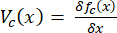
Introduced by Simonyan et al. in 2013, saliency map visualization is one of the earliest and most fundamental gradient-based methods for explaining the predictions of convolutional neural networks27. The main idea is to identify the parts of the input image that most influence the model’s decision by computing the gradient of the class score with respect to the input pixels. Mathematically, this involves the following calculations:
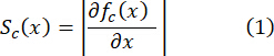
Where fc(x) denotes the score (before softmax) for class c, x is the input. The result is a saliency map Sc(x) that highlights the sensitivity of the class score to changes in each input pixel. To obtain a single two-dimensional map from a multi-channel input, the absolute magnitude of the partial derivatives is computed.
This method is appealing because of its simplicity and model-agnostic implementation, as it does not require architectural modifications or retraining. However, it also suffers from several limitations, such as noisy and visually ambiguous maps, especially in deeper networks; sensitivity to input perturbations that lead to unstable explanations; and a lack of directional insight, which only indicates how much each pixel affects the output.
The Vanilla Gradient method is a straightforward extension of the saliency map technique, in which the raw gradient of the model’s output with respect to the input is used to understand which input features contribute the most to the prediction28. This method offers richer interpretations of the costs of potential noise and sensitivity. It provides directional insights (positive or negative contributions) by considering the gradient’s sign (positive or negative gradient)29. Therefore, what distinguishes the Vanilla Gradient from Saliency Maps is that it preserves the sign of the gradient, allowing not only identification of influential input features but also interpretation of their direction of influence; positive gradients suggest that increasing the input value increases the class score, whereas negative gradients imply the opposite effect.
 (2)
(2)
Integrated gradient
Integrated gradients (IG), introduced by Sundararajan et al. in 2017, is a gradient-based attribution method designed to overcome the limitations of conventional saliency methods, particularly gradient saturation and local sensitivity30. Instead of computing the gradient only at the input point, IG accumulates gradients along a straight-line path from a reference input (baseline) x′ to the original input x. This produces attribution scores that better reflect the cumulative contribution of each feature to the model prediction.
For an input feature xi’ the attribution is defined as:

Where F(⋅) denotes the model output for the target class, x’ is the baseline input, and α interpolates between the baseline and the original input.
Because the integral is incalculable, the definition of integrated Gradients is approximated numerically using a Riemann summation:
 (4)
(4)
Where m denotes the number of interpolation steps. Typical implementations use between 20 and 300 steps, depending on the desired trade-off between computational cost and approximation accuracy.
Unlike conventional gradient methods, Integrated Gradients satisfies several desirable axioms that provide theoretical guarantees for feature attribution. Sensitivity ensures that features influencing the prediction receive non-zero attribution, Implementation Invariance guarantees identical explanations for functionally equivalent networks, and Completeness ensures that the sum of all feature attributions equals the difference between the model outputs at the input and the baseline.
The choice of the baseline is a critical factor affecting the quality of the explanations. While a zero-valued or black image is commonly adopted for natural images, such a baseline may not represent the absence of information in medical imaging. For example, in computed tomography (CT), an intensity value of zero corresponds approximately to water on the Hounsfield scale rather than to an empty image, while magnetic resonance imaging (MRI) intensities are also physically meaningful. Consequently, inappropriate baseline selection may introduce misleading attribution patterns and should be carefully adapted to the imaging modality and clinical context.
Integrated gradients provides smoother and more stable attribution maps than conventional saliency methods and is less affected by gradient saturation. However, its computational cost increases with the number of integration steps, and its explanations remain dependent on the selected baseline.
DeepLIFT
Deep Learning Important FeaTures (DeepLiFT) were introduced by Shrikumar et al. in 2017, to address specific challenges such as gradient saturation and zero gradients31 quantifies the contribution of each input feature to the output by comparing neuron activations against a predetermined baseline, rather than relying solely on gradients. Because DeepLiFT depends on a defining baseline input for each feature to determine its impact on the final output, the choice of baseline can significantly influence attribution, and implementations may define or apply baselines differently. Unlike gradient-based methods, DeepLIFT does not rely directly on the gradients of the output with respect to the input. Instead, it utilizes reference-based differences to propagate relevance through the network. This approach makes DeepLIFT particularly useful for sensitive networks or those that may suffer from gradient saturation.
DeepLIFT builds on the idea introduced by the Gradient × Input method31 but improves upon it by comparing activations at the actual input with those at a reference (often a baseline or neutral input), rather than relying solely on gradients. In the Gradient × Input method, saliency maps are obtained by multiplying the gradient of the output with respect to the input by the input itself, which approximates the first-order change in the output when the input is perturbed. This approach is a simple first-order Taylor approximation of how the model output changes if the input is set to zero. DeepLIFT improves this by using activation differences, making it more robust, particularly in situations where gradients are saturated or near zero.
Input×gradient, as a gradient-based method, computes attributions by multiplying the input values by the output partial derivatives with respect to the input. Mathematically, for an input vector x= [x1, x2, ..., xn] and the model output f(x), the attribution for each feature xi is given by:
 (5)
(5)
Like Integrated Gradients, DeepLIFT relies on a reference baseline to estimate feature contributions. Consequently, the quality and clinical relevance of the generated explanations strongly depend on the appropriateness of the chosen baseline. In medical imaging, a zero-valued baseline may not indicate the absence of anatomical information; for example, in CT, zero represents water rather than an empty image, making modality-specific baseline selection an important consideration.
DeconvNet
In 2014, Zeiler and Fergus introduced a method known as Deconvolutional Networks (DeconvNet) to better understand how convolutional neural networks (CNNs) process visual information32. Their aim was to map feature activities in the intermediate layers, showing which patterns or structures in the input image are responsible for activating specific neurons. Unlike methods that focus directly on the network's output, DeconvNet provides a window into the model's internal hierarchical representations. DeconvNet is structured to operate similarly to convolutional networks, using the same components (filtering and pooling) but in reverse (Figure 4 illustrates the procedure). Reverse propagation is achieved in three main steps:
Unpooling: During the forward pass, max-pooling reduces the spatial dimensions by retaining only the strongest activations. DeconvNet reverses this step by placing the activation back to its original position using the stored pooling indices.
Rectification: A modified (Rectified Linear Unit (ReLU) function was applied during the backward pass, allowing only positive gradients to propagate while suppressing negative ones. This rectification step filters irrelevant signals and enhances the clarity of the reconstructed visualization.
Filtering: using the transposed versions of the learned convolutional filters. This filtering operation reconstructs lower-level feature representations from higher-level activations and progressively traces the visual patterns that activate the selected neuron. Unlike the forward convolution, no new parameters are learned during this step; the trained convolutional filters are reused in reverse for visualization purposes.
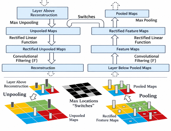
Figure 4. Deconvolutional neural network22. Please click here to view a larger version of this figure.
Guided backpropagation
Guided Backpropagation (GBP) was proposed in 2015 by Springenberg et al.33. This method improves upon Vanilla Gradient and DeconvNet by modifying the backward propagation through Rectified Linear Unit (ReLU) layers. While Vanilla Gradient propagates gradients only through neurons that were active during the forward pass, and DeconvNet propagates only positive incoming gradients, Guided Backpropagation combines both conditions, resulting in more focused and visually interpretable attribution maps.
Let a denote the forward activation before the ReLU function and ggg the incoming gradient during the backward pass. The backward propagation rules for the three methods can be expressed as follows:
Vanilla Gradient:  (a > 0)
DeconvNet: 
Guided Backpropagation: 
Where 1(⋅) denotes the indicator function
The core idea of Guided Backpropagation is therefore to introduce a double-gating mechanism during the backward pass: gradients are propagated only when the neuron was activated during the forward pass, and the incoming gradient is positive. This selective filtering suppresses noisy or irrelevant negative signals, producing a sharper, more localized visualization of the image regions that contribute to the prediction.
Unlike DeconvNet, which constructs visual features via transposed convolutions, Guided Backpropagation operates directly on the original network by modifying only the backward ReLU operation. Consequently, it does not require architectural changes and can be readily applied to a wide range of neural network models.
Layer-wise relevance propagation (LRP)
Layer-wise relevance propagation (LRP), introduced by Bach et al.34, explains the prediction of a trained neural network by decomposing its output into relevance scores assigned to each input feature. Rather than relying on local gradients, LRP redistributes the prediction score backward through the network using predefined propagation rules, thereby quantifying each neuron's contribution to the final prediction. The resulting relevance scores indicate the extent to which individual input features support or oppose the predicted class.
The fundamental principle of LRP is the relevance conservation rule, whereby the relevance assigned to a neuron is redistributed to neurons in the preceding layer according to specific propagation rules. Under the basic LRP formulation (LRP-0), the total relevance is conserved across successive layers, such that the sum of the relevance scores remains equal to the prediction score. However, this conservation property does not hold exactly for all LRP variants. For example, the widely used LRP-ε rule introduces a stabilizing term to avoid numerical instabilities, while bias terms may also absorb part of the propagated relevance. Consequently, relevance conservation is only approximate for these variants and depends on the selected propagation rule.
An important theoretical result reported by Ancona et al.35 demonstrates that several attribution methods are closely related. LRP-0 is mathematically equivalent to Gradient × Input for ReLU networks, while DeepLIFT using the Rescale rule with a zero baseline produces equivalent relevance scores under the same assumptions. These equivalences provide a unified theoretical perspective on gradient- and relevance-based attribution methods, highlighting that their differences often stem from the adopted propagation rules rather than from fundamentally different explanatory principles.
LRP has been extensively applied in medical imaging29,36, where it has demonstrated the ability to identify clinically meaningful regions consistent with expert annotations. Its class-specific and semantically informative heatmaps make it a valuable tool for interpreting deep neural networks in safety-critical applications. Nevertheless, LRP also presents several limitations. It requires customized backward propagation rules that are not natively supported by all deep learning frameworks, and the quality of the generated explanations depends strongly on the selected propagation rule. Furthermore, the interpretation of negative relevance values remains an open research question, particularly in complex clinical decision-making scenarios.
Class activation maps (CAM)
Another important family of backpropagation-based explainability methods is Class Activation Mapping (CAM), which aims to identify the spatial regions in an input image that contribute most to the prediction of a target class. Introduced by Zhou et al.37 in 2016, the original CAM method requires modifying the architecture of a convolutional neural network (CNN) by replacing the fully connected layers with a Global Average Pooling (GAP) layer applied to the feature maps of the last convolutional layer. The GAP layer computes a single activation value for each feature map, and the resulting class activation map is obtained as a weighted linear combination of these feature maps:

Where Ak(x,y) denotes the k-th feature map of the last convolutional layer at spatial location(x,y) and  is the weight connecting feature map k. The resulting heatmap highlights the image regions that contribute most strongly to predicting the target class.
Although CAM provides intuitive class-discriminative visualizations, its main limitation is its architectural dependency. Specifically, it can only be applied to CNNs containing a GAP layer immediately before the classification layer, making it unsuitable for many pre-trained models that employ fully connected layers after the convolutional blocks.
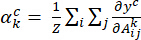
To overcome this limitation, Gradient-weighted Class Activation Mapping (Grad-CAM) was proposed by Selvaraju et al.38. Unlike CAM, Grad-CAM can be applied to a wide range of CNN architectures without requiring architectural modifications. Instead of using the classifier weights directly, Grad-CAM computes the importance of each feature map by averaging the gradients of the target-class score with respect to that map.
 (7)
(7)
Where yc is the score of the target class Aijk represents the activation at spatial location (i,j) of feature map k, and Z is the total number of spatial locations. These importance weights are then used to construct the class activation map.
Despite its flexibility and widespread adoption, Grad-CAM has several limitations. First, because it relies on the last convolutional layer, the resulting heatmaps have a relatively coarse spatial resolution and must be upsampled to the original image size, which can reduce localization accuracy. Second, Grad-CAM may fail to accurately localize multiple instances of the same class, often highlighting only the most dominant object. Finally, the final ReLU discards negative evidence, preventing visualization of image regions that inhibit the predicted class.
Several extensions have been proposed to address these limitations. Grad-CAM++39, one of the most widely used explainability methods in medical imaging, refines the computation of the feature-map weights by incorporating pixel-wise gradient information, enabling improved localization of multiple object instances and producing more precise attribution maps. Furthermore, Guided Grad-CAM38 combines the high spatial resolution of Guided Backpropagation with the class-discriminative localization of Grad-CAM. By fusing these complementary explanations, Guided Grad-CAM generates detailed visualizations that preserve fine-grained image structures while emphasizing the regions that contribute to the model's prediction. Figure 5 outlines the evolution of CAM-based backpropagation methods.
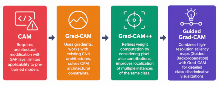
Figure 5. The evolution of CAM-based backpropagation explainability methods. Abbreviations: CAM = Class Activation Mapping; GRAD-CAM = Gradient-weighted CAM. Please click here to view a larger version of this figure.
Perturbation-based methods
These methods assess the impact of localized, small changes in the input features on the model's output. These changes can be implemented by masking, removing, or altering specific input features. After each perturbation, the model's prediction was evaluated. The change in the model output owing to the applied perturbation can be represented as
 (8)
(8)
Where x: a given input, f: the model’s prediction, and δ: the perturbation vector.
Therefore, Δy, which represents the difference between predictions, quantifies the model's sensitivity to the perturbation. A large Δy indicates that the perturbed region is important for the prediction of the model, whereas a small Δy suggests a minimal impact. The sign of Δy indicates the direction of the prediction; a positive Δy (Δy > 0) suggests that the perturbation reinforces or increases the prediction, whereas a negative Δy (Δy < 0) indicates that the perturbation weakens or decreases the prediction.
Occlusion sensitivity map
Among perturbation-based explainability methods, Occlusion Sensitivity is one of the simplest and most intuitive techniques for identifying the contribution of different image regions to a model's prediction. Proposed by Zeiler and Fergus32 in 2014, this method systematically masks a small region of the input image with a predefined patch (typically gray or black) and measures the resulting change in the model's prediction score. By repeating this process over the entire image, an importance map is generated, highlighting the regions that most influence the model's decision.
Although equation (8) defines the perturbation effect as the change in prediction score after applying a perturbation, occlusion sensitivity maps are conventionally visualized using the opposite sign, that is, as the decrease in the target class score after masking a region:

Where xoccluded denotes the input image after masking the local region. Under this n, larger positive values indicate that occluding the corresponding region produces a greater reduction in the prediction score, implying that the region is more relevant to the model's decision.
Occlusion Sensitivity is a model-agnostic method because it does not require access to the model's internal architecture or parameters. Instead, it treats the model as a black box and evaluates the effect of perturbing individual input regions solely through repeated forward passes. However, this exhaustive evaluation is computationally expensive, as each occluded region requires a separate inference. Consequently, generating high-resolution occlusion maps may require hundreds or even thousands of forward passes for a single image, making the method significantly slower than gradient-based approaches23.
Local interpretable model-agnostic explanation LIME
LIME40 is another perturbation-based method that uses a comparative approach to occlusion, in addition to a simpler, interpretable surrogate model to explain individual predictions (local explainability), to create a blackbox model. The surrogate model aims to approximate the behavior of the primary model around a specific input. It can be a linear regression or a decision tree. LIME’s sub-steps start by generating a perturbed version for a specific instance by altering the so-called super-pixels that can be of any arbitrary shape. The model predictions for these altered instances were then used to train a surrogate model that replicates the original model's behavior around each instance. LIME analyzes the surrogate model to identify the most influential features for prediction, resulting in a localized and interpretable explanation of the model's choice. The weights of the features in the local interpretable model represent their importance in explaining the blackbox model's prediction of the original data.
LIME is also an agnostic method that explains the predictions of any type of machine-learning model (e.g., deep neural networks, support vector machines). Furthermore, it provides localized, detailed explanations for individual predictions, offering insights into the model's behavior in the vicinity of that point. However, its main limitations are the instability in explanations owing to randomness in perturbations and the high computational cost for generating and analyzing perturbations.
SHapley Addiditive exPlanations SHAP
In 2017, Lundberg and Lee41 introduced the SHAP (SHapley Additive exPlanations) method, which provides consistent and mathematically sound explanations for machine-learning model predictions. SHAP’s strategy is based on cooperative game theory, particularly the concept of Shapley values, to fairly estimate the “contribution” of each feature towards the model's output. In cooperative game theory, Shapley values are used to allocate payouts among players based on their contributions to the total outcome. SHAP adapts this concept to blackbox prediction models (machine learning) by treating the input features as players and the model’s prediction as the payout.
In technical terms, the input features are grouped into coalitions that reflect which features are included (present) or excluded (absent) in a particular evaluation. The presence or absence of features in each coalition was systematically examined to explore the model for 2n possible feature coalitions (where n is the number of input features) which becomes computationally prohibitive for high-dimensional inputs such as medical images28, and it is precisely this computational bottleneck that motivates the need for approximation methods like KernelSHAP. The Shapley value for feature i is defined as the average marginal contribution of that feature across all possible feature subsets:
 (10)
(10)
Where N denotes the total number of features, S is a subset of features not containing i. f(S) is the model's prediction when only features in S are present.
Using this foundation, SHAP can provide not only local explanations but also the global interpretability of the model. By aggregating the Shapley values across multiple instances, SHAP identified the average importance of each feature and its interaction effects in the model. These global explanations help build trust in the model by revealing the features that it consistently relies on across the dataset, ensuring transparency and alignment with domain knowledge. Additionally, they help identify biases or inconsistencies in the model's behavior, enabling stakeholders to detect and address potential issues that could undermine fairness or reliability. Nevertheless, SHAP's dual focus on local and global explanations can increase computational costs, making it less applicable to time-sensitive or resource-constrained fields. In the same paper41, Lundberg and Lee introduced KernelSHAP to efficiently approximate Shapley values (game-theoretic credit allocation scores) to explain individual predictions of any complex machine learning model without needing to evaluate the model on every feature subset. KernelSHAP frames this approximation within the LIME framework, in which LIME’s local surrogate model is a weighted linear regression. By choosing a particular kernel, loss function, and regularizer within that framework, the traditional LIME heuristics are mathematically overridden, forcing the local linear regression to recover the exact Shapley values.
Score-CAM
Introduced by Wang et al. in 2020, Score-CAM is a visual explanation method that draws inspiration from the CAM lineage while removing gradient dependency42. It bridges the gap between perturbation-based and CAM-based methods and intuitively represents the weights of activation maps. Unlike Grad-CAM and its variants, which rely on gradients to compute channel weights, Score-CAM uses a forward-pass approach to evaluate the importance of each feature map. As illustrated in Figure 6, the activation maps extracted from the last convolutional layer are first upsampled to the size of the input image. Each upsampled activation map is then used as a mask and multiplied elementwise with the original image to generate a masked input. This masked image is then forwarded through the network, and the resulting target-class score is used as the importance weight for the corresponding activation map. The final class activation map is obtained as a weighted linear combination of all activation maps, with weights that reflect each channel's contribution to the prediction.
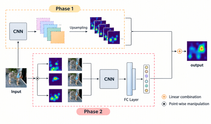
Figure 6. Pipeline of Score-CAM28. Abbreviations: CAM = Class Activation Mapping; CNN = convolutional neural network. Please click here to view a larger version of this figure.
Comparative analysis of XAI methods
The choice between perturbation-based and backpropagation-based XAI techniques depends on several factors, including model architecture, computational efficiency, interpretability, robustness, and explanation faithfulness. Table 1 provides a comparative overview of these two families of XAI methods, highlighting their applicability, computational characteristics, interpretability, scalability, and evidence regarding the reliability of their explanations in medical imaging. As summarized in Table 1, perturbation-based methods provide model-agnostic explanations and are applicable to any predictive model, making them attractive for heterogeneous clinical applications. Their ability to directly evaluate the influence of image regions often yields intuitive, highly localized explanations. However, these methods require repeated perturbations and multiple forward passes through the model, leading to high computational costs and limited scalability, particularly for high-resolution medical imaging modalities such as CT and MRI. Furthermore, methods based on random sampling, such as LIME and SHAP, may produce explanations that vary across runs, potentially affecting their reproducibility in clinical practice.
| Criterion | Perturbation-Based Methods | Backpropagation-Based Methods | |||
| Basic Principle | Perturb the input (e.g., masking, occlusion, noise) and measure the impact on the model prediction. | Compute feature importance by propagating gradients or activation information through the network. | |||
| Representative Methods | Occlusion, LIME, SHAP, Score-CAM | Saliency Maps, Gradient × Input, Integrated Gradients, Grad-CAM, Guided Backpropagation, Guided Grad-CAM | |||
| Model Dependency | Model-agnostic; applicable to virtually any predictive model. | Model-specific; requires differentiable neural network architectures. | |||
| Spatial Resolution | Patch-/superpixel-dependent [1] | Varies by method. Gradient-based methods provide pixel-level attribution, whereas Grad-CAM produces coarse localization maps based on convolutional feature maps. | |||
| Computational Cost | High; requires multiple forward passes for each explanation. | Low; typically requires a single forward and backward pass. | |||
| Scalability | Limited for high-resolution medical images because of repeated perturbations. | Highly scalable and suitable for large CNN models and real-time applications. | |||
| Robustness to Gradient Noise | Gradient-independent [2] | May be affected by gradient saturation, noisy gradients, or vanishing gradients depending on the method | |||
| Interpretability | Generally intuitive because explanations are directly linked to input perturbations. | Depends on the attribution method and requires understanding of gradient propagation. | |||
| Faithfulness | Explanations are generated from prediction changes induced by perturbations and are inherently model-dependent. | Method-dependent. Gradient-based methods such as Grad-CAM and Integrated Gradients exhibit greater sensitivity to model parameters, whereas Guided Backpropagation, DeconvNet, and Guided Grad-CAM have been shown to fail model- and data-randomization sanity checks, potentially producing class-insensitive explanations. | |||
| Clinical Suitability | Well suited for detailed offline analysis where computational cost is acceptable. | Well suited for real-time clinical support; however, explanation faithfulness should be considered when selecting a method for safety-critical applications. | |||
Table 1. Key characteristics of perturbation-based and backpropagation-based methods. 1 Spatial resolution depends on the perturbation granularity, such as the patch size in Occlusion Sensitivity and the superpixel segmentation used in LIME. Therefore, perturbation-based methods do not inherently provide pixel-level localization. 2 Perturbation-based methods are independent of gradient noise. However, sampling-based approaches such as LIME and KernelSHAP may exhibit variability across repeated runs due to stochastic sampling. Abbreviations: LIME = Local Interpretable Model-Agnostic Explanation; SHAP = SHapley Addiditive exPlanations.
Conversely, backpropagation-based methods are computationally efficient and highly scalable. Consequently, they are well-suited for deep convolutional neural networks and real-time clinical decision support. Nevertheless, their effectiveness depends on differentiable model architectures, and they remain susceptible to issues such as gradient saturation, noisy gradients, and vanishing gradients, which may influence the stability and quality of the resulting attribution maps.
Beyond computational considerations, many studies have highlighted that visual quality alone is insufficient to assess the reliability of XAI methods. Adebayo et al.43 introduced sanity checks based on model parameter randomization and label randomization, demonstrating that several modified backpropagation methods, including Guided Backpropagation and Guided Grad-CAM, remain largely unchanged after the learned model is randomized, suggesting that these explanations are weakly dependent on the model itself. Nie et al.44 further provided a theoretical explanation for this phenomenon, showing that Guided Backpropagation and DeconvNet primarily reconstruct only partial input rather than produce class-discriminative explanations. Subsequently, Sixt et al.45 extended these findings by showing that many modified backpropagation attribution methods, such as LRP, DeepLIFT, and Guided Backpropagation, fail to faithfully reflect the decision-making process of deep neural networks. Collectively, these studies establish explanation faithfulness as an essential criterion for evaluating XAI methods, alongside interpretability and computational efficiency.
Overall, perturbation-based methods remain valuable when high-quality, model-agnostic explanations are required, and computational cost is not a limiting factor. In contrast, gradient-based techniques such as Grad-CAM and Integrated Gradients offer an effective balance between computational efficiency and clinically meaningful visualization, making them suitable for many deep learning applications in medical imaging. However, modified backpropagation approaches, including Guided Backpropagation and Guided Grad-CAM, should be interpreted with caution because visually appealing explanations do not necessarily correspond to faithful representations of the model's reasoning. Consequently, the selection of an XAI method should consider not only computational efficiency and visual interpretability but also the faithfulness of the generated explanations, the underlying model architecture, and the specific clinical objective.
Furthermore, qualitative visual assessment should be complemented by quantitative evaluation protocols to determine whether explanations are both clinically meaningful and faithful to the underlying model. When ground-truth anatomical or lesion annotations are available, localization-based metrics such as Intersection over Union (IoU) and Dice similarity can quantify the spatial agreement between an explanation map and the target region. However, such metrics are not universally applicable because clinically relevant regions may not always be precisely annotated, and a high spatial overlap does not necessarily guarantee faithfulness to the model's decision process. Therefore, localization accuracy should be considered alongside model-based evaluation protocols, such as perturbation tests and model- or data-randomization sanity checks, rather than as a standalone measure of explanation quality.
Challenges and future directions
Despite the wide variety of explainable artificial intelligence (XAI) methods available for AI-based systems, several challenges continue to hinder their widespread adoption in clinical practice. The main challenges affecting the clinical adoption of XAI, along with the emerging research directions proposed to address them, are summarized in Figure 7.
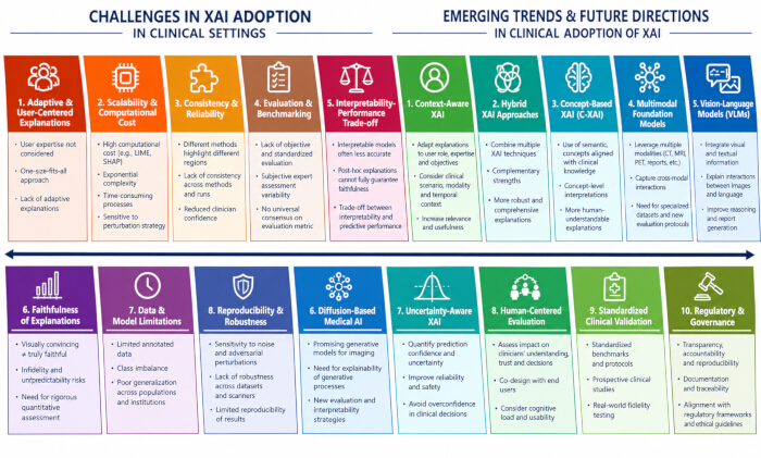
Figure 7. Challenges and emerging directions in the clinical adoption of XAI. Abbreviation: XAI = explainable AI. Please click here to view a larger version of this figure.
One of the primary limitations is the lack of adaptive explanations. Most existing XAI methods generate explanations in a generic manner without considering the diverse backgrounds, expertise levels, or information needs of different users. Consequently, the same explanation may be insufficiently informative for clinicians while being overly technical for non-expert users. As discussed by Yang et al.46, future XAI systems should be capable of tailoring explanations according to the user's role, experience, and clinical objectives.
Another important challenge concerns the scalability of XAI methods. As AI models become increasingly complex and are trained on progressively larger medical datasets, explanation methods also become more computationally demanding47. This limitation is particularly evident in perturbation-based approaches, which require numerous forward passes through the predictive model. For example, local explanation methods such as LIME48 and SHAP49 generate explanations by repeatedly perturbing the input image and observing the resulting changes in the prediction. In medical imaging, these perturbations are typically applied to image segments or superpixels, requiring a large number of model evaluations. For SHAP, the exact computation of Shapley values requires considering all possible feature subsets, resulting in exponential complexity of 2n, where n denotes the number of input features. Consequently, these approaches become computationally expensive for high-resolution modalities such as CT and MRI. Moreover, determining the appropriate perturbation strategy is itself a challenging task, and sampling-based approaches may produce inconsistent explanations across repeated runs50. Another significant challenge is the consistency of explanations. As reported by Wang et al.42, different XAI methods applied to the same trained model frequently highlight distinct image regions, raising important questions about which explanation is most reliable or clinically meaningful. This variability complicates the interpretation of model decisions and reduces clinicians' confidence in XAI-assisted diagnostic systems.
The ever-increasing use of XAI techniques in medical imaging has created a need to evaluate the quality and reliability of these explanations51. Although expert assessment is valuable, it is often affected by inter- and intra-observer variability, making purely subjective evaluation insufficient. Consequently, several quantitative evaluation protocols have been proposed to objectively assess different properties of attribution methods. Among the most widely adopted are deletion and insertion tests52, which evaluate the effect of progressively removing or adding highly attributed image regions on the model prediction. The Pointing Game53 measures whether the most salient region correctly overlaps with any ground truth region. It works by checking whether the pixel with the maximum activation value in a saliency map lies within the object's ground-truth bounding box and then calculating an overall localization accuracy score based on these binary hits and misses. ROAR (Remove And Retrain)54, is another evaluation protocol that evaluates feature importance by retraining the model after removing highly attributed regions. It assesses whether the features identified by an explanation are important for the model's predictive performance. However, retraining a deep learning model for each fraction of features removed requires substantial time and computational resources. Recent studies show that pixel-based removal can warp data manifolds or leak unintended clues, prompting newer feature perturbation metrics, such as GOAR (Geometric Remove-and-Retrain)55, to propose alternative adjustments. Multiple other researchers have proposed diverse approaches to evaluate the infidelity34,56,57,58 and the faithfulness58,59 of different XAI methods. Recent studies have further emphasized that visually convincing explanations do not necessarily imply faithful explanations. Arun et al.60 demonstrated that commonly used saliency methods often exhibit limited localization accuracy when compared with expert radiologist annotations, highlighting the importance of quantitative validation before clinical deployment. Furthermore, Rudin61 argued that whenever an inherently interpretable model can achieve predictive performance comparable to that of a blackbox model, it should be preferred to relying solely on post hoc explanations. In medical imaging, however, deep learning models frequently outperform simpler interpretable models for complex diagnostic tasks. Consequently, post hoc XAI methods remain valuable, although their explanations should be interpreted with caution and validated through rigorous quantitative and clinical evaluation protocols.
Although these evaluation protocols have become standard tools for assessing explanation quality, they capture complementary aspects of explainability rather than providing a single comprehensive measure. Therefore, while several robust evaluation frameworks are available, no universal consensus currently exists on a single evaluation metric, making comparisons of XAI methods across studies particularly challenging. In addressing this challenge, recent literature has advocated advanced meta-evaluation frameworks to quantify how accurately a metric reflects true model behavior62.
Several promising research directions may help overcome these limitations. One important direction is the development of context-aware XAI, capable of adapting explanations to the clinical scenario, imaging modality, temporal context, and user profile29. Another promising avenue is the design of hybrid explainability frameworks that integrate complementary explanation techniques to improve robustness, faithfulness, and interpretability while preserving predictive performance. Future research should also focus on establishing standardized evaluation benchmarks that integrate quantitative metrics with expert clinical assessment to enable fair comparisons between XAI methods.
Beyond the methods discussed in this review, emerging explainability paradigms offer additional opportunities for medical imaging. Concept-based XAI (C-XAI) is an emerging direction that aims to explain AI predictions using human-interpretable semantic concepts rather than solely through pixel- or feature-level importance. Recent studies have explored different types of concepts63, richer concept representations, and concept-level interventions, providing opportunities for more meaningful and fine-grained understanding of model behavior. Future research should investigate the integration of C-XAI into medical imaging, particularly for representing clinically meaningful concepts and their relationships, and for developing reliable methods to evaluate and control concept-based explanations. The increasing adoption of multimodal foundation models in medical imaging also introduces new explainability challenges, as these models can integrate heterogeneous information from various sources, and understanding which factors led to a particular diagnosis is essential for clinicians64. Integrating multimodal explanation techniques introduces significant complexities due to the intricate interactions between different data types, such as text and images, making it difficult to isolate each modality's impact on model outputs. This challenge is further compounded by a critical lack of standardized evaluation metrics to assess explanation quality and a scarcity of specialized datasets needed for robust training. Furthermore, systems must overcome barriers to personalization and accessibility to ensure these complex, cross-modal explanations remain clear, useful, and adaptable for both technical experts and non-expert users65. Similarly, vision-language models require explanation mechanisms that clarify the interactions between visual and textual information underlying their predictions or generated outputs. The primary difficulty lies in ensuring that attribution maps, cross-modal attention mechanisms, and text-based rationales faithfully reflect true internal-model reasoning rather than merely producing plausible illusions of interpretability. Diffusion-based medical AI represents another emerging direction, particularly for image generation, reconstruction, and enhancement, where the interpretability of the generative process and the reliability of generated content remain important open questions66.
Another important direction is the development of uncertainty-aware explanations that explicitly communicate the reliability or confidence associated with both predictions and explanations. Such approaches may be particularly valuable in clinical settings, where an explanation without an indication of uncertainty could create a false sense of confidence. In parallel, future XAI systems should increasingly incorporate human-centered evaluation, assessing not only whether explanations are technically faithful but also whether they improve clinicians' understanding, decision-making, and trust. However, implementing a human-centered design approach to create transparent machine learning (ML) tools for high-stakes fields like healthcare is challenging. Key hurdles include communication gaps between developers and medical staff, strict privacy and ethical rules that impede user testing, complex clinical data, and a lack of human-centered design training for machine learning creators67. Finally, regulatory and governance considerations will become increasingly important as XAI systems move toward clinical deployment.
Future research should therefore address the requirements for transparency, accountability, reproducibility, validation, and documentation to support the development of trustworthy and clinically deployable AI systems. Extensive prospective clinical validation and real-world deployment studies are needed to determine whether explainable AI genuinely improves diagnostic decision-making, physician trust, and patient outcomes in routine clinical practice.
Schlussfolgerungen
Ensuring explainability in AI-based systems has become a critical necessity, particularly in high-stakes domains, such as healthcare. For instance, in medical imaging, an AI system might flag a region in a scan as malignant with high accuracy. Without XAI, clinicians may hesitate to rely on these results because of the opacity of the system. Such cases require clear justifications to support clinical decision-making, where the consequences can mean life and death. Consequently, XAI methods enable stakeholders to justify and trust predictions, allowing them to understand the rationale behind the system’s outputs. They address this by highlighting specific features or patterns in the image that inform the decision, thereby aligning the AI model's reasoning with the clinician’s expertise. Because XAI methods can explain how and why the AI-based system makes decisions, they allow clinicians not only to understand the system’s reasoning but also to identify problems and potential biases. For example, if an AI-based system focuses on irrelevant features or biased information, clinicians can address this issue. Therefore, the explanatory goals of XAI methods go beyond simply providing insights into the system's internal working processes. Several XAI methods are presented in this paper and grouped into two categories: perturbation-based and backpropagation-based methods, each with its own foundational principles. While perturbation-based methods focus on slightly modifying the input data and observing how the AI-based system’s output changes to understand which region of the data has the greatest impact on predictions, backpropagation-based methods basically use gradients to trace the AI's decision-making process backward through the model to identify the features or patterns in the input that contribute the most to its predictions. Each category encompasses a variety of detailed methods, providing specific methods for achieving explainability within backpropagation and perturbation-based frameworks. These methods are indeed gaining prominence in medical imaging research, as evidenced by the growing number of studies addressing explainability. However, their real-world adoption in the healthcare sector remains limited due to several challenges. Consequently, this study attempts to detail the different XAI methods and the major challenges and limitations that currently exist.
Offenlegungen
The authors have no conflicts of interest to declare.
Danksagungen
The authors extend their appreciation to the Deanship of Scientific Research and Libraries in Princess Nourah bint Abdulrahman University for funding this research work through the Supporting Publication in Review Article Program, Grant No. (RAP-2026-92).
Referenzen
- Sayyad L, Sultanabanu K, Sayyad KL. Electronics with artificial intelligence creating a smarter future: a review. J Commun Eng Its Innov. 2023;9(3):38-42.
- Xu Y, et al. Artificial intelligence: a powerful paradigm for scientific research. Innovation (Camb). 2021;2(4):100179.
- Benjamens S, Dhunnoo P, Mesko B. The state of artificial intelligence-based FDA-approved medical devices and algorithms: an online database. NPJ Digit Med. 2020;3(1):118.
- Gao Z, et al. Robust deep learning from incomplete annotation for accurate lung nodule detection. Comput Biol Med. 2024;173:108361.
- Hao Y, et al. Machine learning for predicting the survival in osteosarcoma patients: analysis based on American and Hebei Province cohort. Biomol Biomed. 2023;23(5):883-93.
- Khosravi M, Zare Z, Mojtabaeian SM, Izadi R. Artificial intelligence and decision-making in healthcare: a thematic analysis of a systematic review of reviews. Health Serv Res Manag Epidemiol. 2024;11:23333928241234863.
- Hassija V, et al. Interpreting blackbox models: a review on explainable artificial intelligence. Cognit Comput. 2024;16(1):45-74.
- Xu F, et al. Explainable AI: a brief survey on history, research areas, approaches and challenges. In: Natural Language Processing and Chinese Computing. Lecture Notes in Computer Science. Springer; Cham; 2019. p. 299-318.
- Chaddad A, Peng J, Xu J, Bouridane A. Survey of explainable AI techniques in healthcare. Sensors (Basel). 2023;23(2):634.
- Borys K, et al. Explainable AI in medical imaging: an overview for clinical practitioners—beyond saliency-based XAI approaches. Eur J Radiol. 2023;162:110786.
- Bhati D, Neha F, Amiruzzaman M. A survey on explainable artificial intelligence (XAI) techniques for visualizing deep learning models in medical imaging. J Imaging. 2024;10(10):239.
- Ahmed F, et al. Explainable artificial intelligence (XAI) in medical imaging: a systematic review of techniques, applications, and challenges. BMC Med Imaging. 2026;26(1):37.
- El Amrani W. Attention and beyond: explainability techniques for vision transformers [conference paper]. Presented at: Explain'AI: Knowledge Extraction and Management; Strasbourg, France; 2025.
- Poeta E, et al. Concept-based explainable artificial intelligence: a survey. ACM Comput Surv. 2025. doi:10.1145/3774643.
- Chaddad A, Hu Y, Wu Y, Wen B, Kateb R. Generalizable and explainable deep learning for medical image computing: an overview. Curr Opin Biomed Eng. 2023;28:100485.
- Cheng Z, et al. A comprehensive review of explainable artificial intelligence (XAI) in computer vision. Sensors (Basel). 2025;25(13):4166.
- Stiglic G, et al. Interpretability of machine learning-based prediction models in healthcare. Wiley Interdiscip Rev Data Min Knowl Discov. 2020;10(5):e1379.
- li S, et al. Explainable artificial intelligence (XAI): what we know and what is left to attain trustworthy artificial intelligence. Inf Fusion. 2023;99:101805.
- Agarwal R, et al. Neural additive models: interpretable machine learning with neural nets. Adv Neural Inf Process Syst. 2021;34:4699-711.
- Natekar P, Kori A, Krishnamurthi G. Demystifying brain tumor segmentation networks: interpretability and uncertainty analysis. Front Comput Neurosci. 2020;14:6.
- van der Velden BHM, Kuijf HJ, Gilhuijs KGA, Viergever MA. Explainable artificial intelligence (XAI) in deep learning-based medical image analysis. Med Image Anal. 2022;79:102470.
- Zhang Z, et al. MDNet: a semantically and visually interpretable medical image diagnosis network [conference paper]. Presented at: IEEE Conference on Computer Vision and Pattern Recognition (CVPR); 2017. p. 6428-36.
- Ancona M, Ceolini E, Öztireli C, Gross M. Towards better understanding of gradient-based attribution methods for deep neural networks [conference paper]. Presented at: 6th International Conference on Learning Representations (ICLR); Vancouver, Canada; 2018.
- Ghnemat R, Alodibat S, Abu Al-Haija Q. Explainable artificial intelligence (XAI) for deep learning based medical imaging classification. J Imaging. 2023;9(9):177.
- Patrício C, Neves JC, Teixeira LF. Explainable deep learning methods in medical image classification: a survey. ACM Comput Surv. 2024;56(4):85:1-85:41.
- Singh A, Sengupta S, Lakshminarayanan V. Explainable deep learning models in medical image analysis. J Imaging. 2020;6(6):52.
- Simonyan K, Vedaldi A, Zisserman A. Deep inside convolutional networks: visualising image classification models and saliency maps [conference paper]. Presented at: 2nd International Conference on Learning Representations (ICLR), Workshop Track; Banff, Canada; 2014.
- Molnar C. Interpretable machine learning [Internet]. 2022 [cited 2022 Apr 12]. Available from: https://christophm.github.io/interpretable-ml-book/
- Ahmed MA, Ali L. Explainable medical image segmentation via generative adversarial networks and layer-wise relevance propagation. Nord Mach Intell. 2021;1:20-2.
- Sundararajan M, Taly A, Yan Q. Axiomatic attribution for deep networks [conference paper]. Presented at: 34th International Conference on Machine Learning; Sydney, Australia; 2017. Proc Mach Learn Res. 70:3319-28.
- Shrikumar A, Greenside P, Kundaje A. Learning important features through propagating activation differences [conference paper]. Presented at: 34th International Conference on Machine Learning; Sydney, Australia; 2017. p. 3145-53.
- Zeiler MD, Fergus R. Visualizing and understanding convolutional networks. In: Fleet D, Pajdla T, Schiele B, Tuytelaars T, editors. Computer Vision–ECCV 2014. Springer; Cham; 2014. p. 818-33.
- Springenberg JT, Dosovitskiy A, Brox T, Riedmiller M. Striving for simplicity: the all convolutional net [conference paper]. Presented at: International Conference on Learning Representations (ICLR), Workshop Track; 2015.
- Bach S, et al. On pixel-wise explanations for non-linear classifier decisions by layer-wise relevance propagation. PLoS One. 2015;10(7):e0130140.
- Ancona M, Ceolini E, Öztireli C, Gross M. Gradient-based attribution methods. In: Samek W, Montavon G, Vedaldi A, Hansen LK, Müller KR, editors. Explainable AI: Interpreting, Explaining and Visualizing Deep Learning. Springer; Cham; 2019. p. 169-91.
- Böhle M, Eitel F, Weygandt M, Ritter K. Layer-wise relevance propagation for explaining deep neural network decisions in MRI-based Alzheimer's disease classification. Front Aging Neurosci. 2019;11:194.
- Zhou B, et al. Learning deep features for discriminative localization [conference paper]. Presented at: IEEE Conference on Computer Vision and Pattern Recognition (CVPR); 2016. p. 2921-9.
- Selvaraju RR, et al. Grad-CAM: visual explanations from deep networks via gradient-based localization [conference paper]. Presented at: IEEE International Conference on Computer Vision; 2017. p. 618-26.
- Chattopadhyay A, Sarkar A, Howlader P, Balasubramanian VN. Grad-CAM++: improved visual explanations for deep convolutional networks [conference paper]. Presented at: 2018 IEEE Winter Conference on Applications of Computer Vision (WACV); 2018. p. 839-47.
- Ribeiro MT, Singh S, Guestrin C. Why should I trust you? Explaining the predictions of any classifier [conference paper]. Presented at: 22nd ACM SIGKDD International Conference on Knowledge Discovery and Data Mining; San Francisco, CA; 2016. p. 1135-44.
- Lundberg SM, Lee SI. A unified approach to interpreting model predictions [conference paper]. Presented at: 31st International Conference on Neural Information Processing Systems; 2017. p. 4768-77.
- Wang H, et al. Score-CAM: score-weighted visual explanations for convolutional neural networks [conference paper]. Presented at: 2020 IEEE/CVF Conference on Computer Vision and Pattern Recognition Workshops (CVPRW); Seattle, WA; 2020. p. 111-19.
- Adebayo J, et al. Sanity checks for saliency maps [conference paper]. Presented at: 32nd International Conference on Neural Information Processing Systems; 2018. p. 9525-36.
- Nie W, Zhang Y, Patel A. A theoretical explanation for perplexing behaviors of backpropagation-based visualizations [conference paper]. Presented at: 35th International Conference on Machine Learning; 2018. p. 3809-18.
- Sixt L, Granz M, Landgraf T. When explanations lie: why many modified BP attributions fail [conference paper]. Presented at: 37th International Conference on Machine Learning; 2020. p. 9046-57.
- Yang W, et al. Survey on explainable AI: from approaches, limitations and applications aspects. Hum Cent Intell Syst. 2023;3:161-88.
- Ahmad MA, Teredesai A, Eckert C. Interpretable machine learning in healthcare [conference paper]. Presented at: 2018 IEEE International Conference on Healthcare Informatics (ICHI); 2018. p. 447.
- Hassan SU, et al. Local interpretable model-agnostic explanation approach for medical imaging analysis: a systematic literature review. Comput Biol Med. 2024;185:109569.
- Husby UE. Exploring breast cancer diagnosis: a study of SHAP and LIME in XAI-driven medical imaging [master's thesis]. Norwegian University of Life Sciences; Ås, Norway; 2024.
- Dazeley R, Vamplew P, Cruz F. Explainable reinforcement learning for broad-XAI: a conceptual framework and survey. arXiv. 2021:2108.09003.
- Markus AF, Kors JA, Rijnbeek PR. The role of explainability in creating trustworthy artificial intelligence for health care: a comprehensive survey of the terminology, design choices, and evaluation strategies. J Biomed Inform. 2021;113:103655.
- Petsiuk V, Das A, Saenko K. RISE: randomized input sampling for explanation of blackbox models. arXiv. 2018:1806.07421.
- Zhang J, et al. Top-down neural attention by excitation backprop. In: Leibe B, Matas J, Sebe N, Welling M, editors. Computer Vision–ECCV 2016. Springer; Cham; 2016. p. 543-59.
- Hooker S, et al. A benchmark for interpretability methods in deep neural networks [conference paper]. Presented at: 33rd Conference on Neural Information Processing Systems (NeurIPS); 2019. Adv Neural Inf Process Syst. 32:9737-48.
- Park YH, Seo J, Park B, Lee S, Jo J. Geometric Remove-and-Retrain (GOAR): coordinate-invariant eXplainable AI assessment. arXiv. 2024:2407.12401.
- Miró-Nicolau M, Jaume-i-Capó A, Moyà-Alcover G. A comprehensive study on fidelity metrics for XAI. Inf Process Manag. 2025;62(1):103900.
- Rieger L, Hansen LK. IROF: a low resource evaluation metric for explanation methods [conference workshop paper]. Presented at: AI for Affordable Healthcare Workshop at ICLR; 2020.
- Bhatt U, Weller A, Moura JMF. Evaluating and aggregating feature-based model explanations [conference paper]. Presented at: 30th International Joint Conference on Artificial Intelligence; 2021. p. 3016-22.
- Alvarez-Melis D, Jaakkola TS. Towards robust interpretability with self-explaining neural networks [conference paper]. Presented at: 32nd Conference on Neural Information Processing Systems; 2018. Adv Neural Inf Process Syst. 31.
- Arun N, et al. Assessing the trustworthiness of saliency maps for localizing abnormalities in medical imaging. Radiol Artif Intell. 2021;3(6):e200267.
- Rudin C. Stop explaining black box machine learning models for high stakes decisions and use interpretable models instead. Nat Mach Intell. 2019;1:206-15.
- Hedström A, et al. The meta-evaluation problem in explainable AI: identifying reliable estimators with MetaQuantus. arXiv. 2023:2302.07265.
- Lee JH, et al. Concept-based explanations in computer vision: where are we and where could we go? In: Del Bue A, Canton C, Pont-Tuset J, Tommasi T, editors. Computer Vision–ECCV 2024 Workshops. Springer; Cham; 2025. p. 251-67.
- Holzinger A, Langs G, Denk H, Zatloukal K, Müller H. Causability and explainability of artificial intelligence in medicine. Wiley Interdiscip Rev Data Min Knowl Discov. 2019;9(4):e1312.
- Giovannoni C, Metta C, Monreale A, Rinzivillo S. A survey on multimodal explainable artificial intelligence. Intell Syst Appl. 2026;31:200671.
- Yaseen M, Ali M, Ali S, Kim HC. Diffusion-based approaches for medical image segmentation: an in-depth review. Electronics (Basel). 2026;15(7):1400.
- Chen H, Gomez C, Huang CM, Unberath M. Explainable medical imaging AI needs human-centered design: guidelines and evidence from a systematic review. NPJ Digit Med. 2022;5(1):156.