Blender as a Tool for Visualization and Animation of the Trypanosome Flagellar Base Using Cryogenic Electron Tomography

Zusammenfassung

Blender is a versatile, free, and open-source graphics software package for rendering three-dimensional models. Here, we describe a workflow for integrating segmentations from cryogenic electron tomography into Blender to generate high-quality scientific visualizations and animations of cellular structures.

Zusammenfassung

Cryogenic electron tomography (cryo-ET) enables three-dimensional visualization of cellular structures and macromolecular assemblies in near-native states. However, tomographic reconstructions and segmented models can be difficult to interpret without effective visualization tools that place structural features within their broader cellular context. This protocol describes a workflow for integrating cryo-ET segmentations with illustrative three-dimensional models in Blender 5.2, a free and open-source platform for modeling, rendering, and animation. The workflow includes preparing segmented volumes, exporting, and importing models, organizing structural components, assigning materials and colors, adjusting lighting and camera settings, and generating keyframe-based animations. In addition to visualizing segmented tomographic data, this workflow also includes building illustrative cellular models that help contextualize structures of interest within the whole-cell architecture. This approach is particularly useful for communicating complex spatial relationships, organelle organization, and dynamic biological processes captured by cryo-ET. By combining experimentally derived segmentations with flexible three-dimensional modeling and animation tools, researchers can create high-quality scientific movies that enhance data interpretation, improve visual communication, and support presentation, publication, and educational applications.

Einleitung

Cryogenic electron tomography (cryo-ET) is a powerful imaging technique that enables three-dimensional reconstruction of biological specimens at sub-nm to sub-micron resolution¹. By computationally aligning and reconstructing a tilt series of projection images, cryo-ET can reveal the spatial organization of cellular structures and macromolecular assemblies in vitrified, near-native states². Because samples are preserved by rapid freezing rather than dehydration or chemical fixation, cryo-ET provides a unique opportunity to visualize cellular architecture with minimal structural perturbation. As cryo-ET datasets become more detailed and complex, effective visualization tools are increasingly important for interpreting structural information and communicating biological mechanisms clearly.

Image processing programs such as Electron Microscopy Analysis 2 (EMAN2) and Image MODeling (IMOD) offer user-friendly platforms for tomogram reconstruction, annotation, and segmentation^2,3,4,5. These tools enable users to identify and label features of interest within tomographic volumes, generating segmented models that can be used for structural interpretation and downstream visualization. In addition, University of California, San Francisco (UCSF) Chimera and ChimeraX provide powerful tools for visualizing molecular structures, density maps, and segmented cellular features^6,7. These programs support functions such as density-map display, fitting, superposition, segmentation, measurement, and basic animation through command-line or Python-based scripting. Together, these platforms are essential for processing and analyzing cryo-ET data.

However, standard tomography and molecular visualization programs are not primarily designed for building illustrative three-dimensional scenes, integrating experimentally derived segmentations with conceptual models, or producing polished animations for broad scientific communication. For many biological questions, segmented structures must be placed within a larger cellular context to explain their spatial relationships, functional organization, and dynamic behavior. This visual context is particularly important when communicating complex cellular processes, where experimentally observed structures may need to be combined with simplified illustrative models to convey the biological concept clearly.

Blender, a computer graphics software made by the Blender Foundation, is a free, open-source three-dimensional modeling, rendering, and animation program that provides extensive tools for scientific visualization^8,9,10,11. Although originally developed for animation, visual effects, and game design, Blender offers features that are highly useful for biological visualization, including flexible mesh editing, material assignment, lighting control, camera movement, keyframe-based animation, and high-quality rendering. These capabilities allow users to create visually engaging models, adjust textures and transparency, control illumination and shadows, and generate smooth camera paths to highlight structures of interest.

Here, we describe a workflow for using Blender to enhance the visualization and animation of cryo-ET segmentation data. The protocol demonstrates how segmented models generated from cryo-ET datasets can be exported and imported into Blender, organized as editable objects, and combined with illustrative three-dimensional cellular models. We further describe how to assign materials, adjust lighting, animate cameras and objects, and generate final scientific movies. This workflow provides an accessible strategy for transforming complex tomographic segmentations into clear, high-quality visualizations that support data interpretation, scientific presentation, publication, and education.

Protokoll

NOTE: Accurate visualization of three-dimensional tomogram segmentations is essential for interpreting complex biological structures and their spatial relationships. This protocol describes how to prepare cryo-ET segmentations generated or processed in EMAN2, IMOD, or Chimera, and use Blender to enhance model presentation, camera positioning, lighting, scene composition, and animation.

1. Exporting segmentations from Chimera and importing them into Blender (Supplementary Video 1, Supplementary Video 2)

NOTE: Before exporting cryo-ET segmentation volumes from Chimera, preprocess the volume to reduce the number of disconnected or fragmented components. This step simplifies downstream animation and allows individual structural elements to be animated or manipulated as cohesive objects.

1. Prepare the segmentation volume in Chimera.
   1. Open the segmentation file in Chimera (Figure 1A).
   2. In the Volume Viewer dialogue (Figure 1B), set the display style to Surface, set Plane to All, and set Step to 1 to display the segmentation as a three-dimensional surface.
   3. Adjust the threshold in Volume Viewer until the desired structural components are clearly visible. For example, for the flagellar axoneme segmentation shown in Figure 1A, a threshold value of 1 reveals individual microtubules within the segmentation.
   4. Set the voxel size of each segmentation map to 1 to ensure consistent scaling and proportions among imported objects.
   5. Center and orient the segmentation to establish a clear reference point for exporting.
2. Export the segmentation from Chimera:
   1. In the model view (Figure 1C), navigate to File > Export Scene.
   2. Select COLLADA (.dae) as the export file type.
   3. Include the .dae file extension in the file name to avoid confusion during import and file organization.
      NOTE: The next step depends on which version is being used. Versions 5.0 and above do not natively import .dae file types. This will instead require either downloading a third-party add-on to support additional file types, or using a third-party website to convert the .dae into a .obj or another accepted file type. Using add-ons is recommended, as there are options available from the official Blender Extension Platform repository that avoid the potential loss of metadata, as described in step 1.3.3. Older versions can natively take .dae files, and step 1.3.3 can be ignored without additional setup.
3. Import the segmentation (Figure 2)
   1. Open Blender (Figure 2A).
   2. Delete the default cube, camera, and light objects to start with a clean scene.
   3. If on Version 5.0 or above:
      1. Search for a DAE extension add-on script.
      2. Download and extract the script.
      3. Go back to the simulation software, select the Edit tab, click Preferences, then Add-ons.
      4. Go to the top right drop-down arrow, click Install from Disk, and select the extension script.
   4. Navigate to File > Import > Collada (.dae), and select the file exported from Chimera (Figure 2B).
   5. After importing the segmentation, check for the imported file in the Scene Collection panel on the right. This may include a camera, light nodes, and an object node, represented by three-dimensional axes.
   6. Select the imported object node and adjust the scale of the X, Y, and Z axes to 0.01 or smaller if needed.
   7. Zoom out to locate the imported segmentation in the Blender viewport (Figure 2C).
   8. Perform further adjustments to the scale to make the segmentation manageable for visualization and animation (Figure 2D).
      NOTE: Blender does not automatically preserve or display the experimentally measured dimensions of imported segmentations. Record the original dimensions in Chimera before importing. Because objects are scaled multiplicatively, these recorded values can be used later to calculate proportional size adjustments and maintain accurate relationships among structures.
4. Organize segmentation objects.
   1. In the Scene Collection panel, locate the imported segmentation objects within the imported axes object folder in the right-hand directory.
   2. Rename each segmentation object according to the corresponding biological structure, such as membrane, or organelle. Clear naming will help with identification and selection of specific components during later editing and animation steps.
   3. If the imported segmentation appears as a single object but needs to be divided into separate structural components, select the object and enter Edit mode to divide it into individual objects.
5. Regroup each segmentation object (Figure 3, Supplementary Video 3).
   1. Enter Edit Mode using the menu at the top left, then select Mesh > Separate, which allows independent manipulation and animation of each component (Figure 3A).
   2. Select the parts of the model that should be separated or regrouped.
   3. Right-click the selected object, choose Separate, and select By Loose Parts. Each stand-alone piece within the original object will now become an individual object (Figure 3B).
   4. To regroup the related object components, return to the Object mode, hold Shift, and select all objects that should be combined (Figure 3C).
   5. Right-click the selected objects and choose Join to merge them into a single object (Figure 3D).
   6. Rename the newly joined object using a descriptive name.
      NOTE: Separating and regrouping objects allows individual structural components to be manipulated independently or animated together. Clear object naming is essential for later steps involving material assignment, camera tracking, and scene organization. Following these steps prepares cryo-ET segmentations for efficient manipulation. Proper preprocessing, scaling, naming, and organization of imported objects provide the foundation for creating informative and visually appealing animations of cellular structures and biological processes.

2. Preparing segmentations for animation (Supplementary Video 4)

NOTE: After importing the segmentation, set up the scene for visualization and animation. This section describes the basic steps for organizing the scene, adjusting model position and scale, applying materials, setting up lighting, and positioning the camera. These steps provide a foundation for generating clear and effective animations of cellular structures.

1. Setting up the animation scene.
   1. To clean up the scene, go to the Scene Collection window in the top right, highlight all default objects in the collection except for the segmentation object, and delete them (x key).
   2. Add a new camera as described in step 2.2.4 and add lighting by selecting the add option from the top left corner of the scene interface and choosing the desired object.
   3. For positioning and scaling, use the Move tool in the toolbar on the left side of the window to position the entire segmentation to the center of the scene. Alternatively, select the desired object and go to the Object tab in the bottom-right properties window. Adjust the values under Transform to make translational movements along the X, Y, or Z axis for the selected object.
      NOTE: Move the segmentation as a whole rather than moving individual parts separately, as independent movement of parts may distort the spatial relationships within the segmentation.
   4. Adjust the scale of the segmentation as needed to make the model easy to view and manipulate. Use the same menu used for scaling during the import process in protocol 1.1.6 (or 1.3.6–1.3.8, as applicable).
   5. Add a ground surface under the model if needed. To do so, go to the Add tab, hover over Mesh, and select Plane. Use the same scaling and translation methods described in step 1.3.6 to scale or translate the plane to the desired size and location. This provides a spatial reference point within the three-dimensional scene and allows the shadow and other spatial features of the model to be visualized.
2. Adjust materials, lighting, and camera position.
   1. To preview the model with full shading and reflections, navigate to the upper-right corner of the model screen, where four spheres representing different shading and coloring modes can be found. Select the rightmost sphere, representing a real-time render of the environment.
      NOTE: Depending on the computer’s processing capacity and the complexity of the model, selecting the rightmost option of shading and reflections active may cause lag. The setup used here for rendering animations and advice for quality optimization is provided in the Discussion section.
   2. To apply the texture and colors, go to the Properties menu in the bottom left, and select the red sphere called Material Properties. Use the Material Properties panel to apply coloring to the model as needed. To highlight structural features, experiment with surface sliders such as Metallic, Roughness, and Alpha to achieve the desired texture (Figure 4A,B).
   3. In particular, use the Alpha slider setting to control the object's transparency. Adjusting Alpha can be useful for temporarily fading selected objects/segmentations, allowing other structures to be viewed more clearly or highlighted within the model (Figure 5A,B).
   4. Add a camera to the scene and position it to capture the model from the desired angle. Adjust the camera location, rotation, and focal length to emphasize the region of interest and improve the visibility of detailed structures.
   5. Add and modify lighting to enhance the appearance of the segmentations. Use the Sun object to illuminate the entire model evenly or use a Spot Light to highlight specific regions or smaller structural components.
      ​NOTE: Adjusting the lighting affects the shadows cast by the segmentations and the ground surface, thereby enhancing depth perception and spatial relationships within the scene. Varying the material properties and lighting conditions can help convey surface features, such as smoothness, roughness, transparency, or reflectivity, and can further emphasize the three-dimensional organization of the segmentation. Together, with optimized lighting and texture settings to accentuate structural details, a more realistic visualization can be produced that directs the viewer’s attention to specific regions of interest, including smaller or more intricate components of the data (Supplementary Video 5).

3. Creating and animating dynamic illustration models (replication animations without tomographic data) (Supplementary Video 6)

NOTE: Blender can additionally be used to create illustrative three-dimensional models that provide cellular context for segmented tomographic data. For example, a whole-cell model of Trypanosoma brucei (T. brucei) can be generated and used to show how segmented structures are positioned within the broader cellular architecture. These illustrative models help connect structural information from cryo-ET with the biological processes in which the structures participate. Figure 6A–D present a basic model of a rendered T. brucei cell undergoing division. The model was created using Editing mode, in which vertices, edges, and faces can be added and modified to generate three-dimensional objects with the desired level of complexity. Blender also offers a range of texture settings, including transparency, sheen, roughness, and surface smoothness, which can be adjusted to control how surfaces interact with light. These features enable the creation of visually rich objects, such as partially opaque models that reveal internal structures, or rounded faces that provide a softer and more natural appearance. Simple keyframing-based animations, such as a gradual fade-in effect or coordinated movement of a daughter cell, can be used to illustrate dynamic biological processes such as cell replication. Dynamic deformation of illustrative models through armature-based rigging is also possible. By attaching a rig to a model, the structure can be bent, stretched, or moved to simulate biological motions, such as flagellar beating, cell-body bending, or replication-associated changes in cell shape. This approach allows users to create animated models that communicate complex biological processes in a visually intuitive format. The following steps describe how to generate a simple armature and attach it to an illustrative model.

1. Create a rigging for an illustration model (Figure 7A).
   1. Add an armature to the scene from the Add tab. A single object will appear, referred to as a bone. This bone serves as the starting point for the model movement. Add additional bones to generate more complex and flexible motion by going into Edit Mode and pressing E (Figure 7B).
   2. Position and rotate the armature so that it begins at the posterior end of the model and extends toward the center of the cell.
   3. To keep the armature visible when it is blocked by other objects, go to the armature object, select Viewport Display settings, and enable In Front.
   4. To extrude additional bones, select the circular nub at the end of the bone and press E to extrude a second bone.
   5. Rotate and position the new bone as needed, then left-click to place it.
   6. Repeat this process to extrude bones toward the anterior end of the model. (Figure 7C).
   7. Now, rig the armature to the model.
      1. Select the mesh, hold shift, and then select the armature.
      2. Press Control + P and select With Automatic Weights. The armature is now automatically rigged to the model. Bone movements will deform the model according to an automatic weighting system based on the position of the bone and the influence of each bone within the model (Figure 7D).
         ​NOTE: If automatic rigging does not produce the desired movement, manually adjust the weighting assigned to each bone. This manual weight-painting process is not covered in this protocol. To refine the rigging, switch to Pose Mode and rotate individual bones to assess how each bone deforms the model. If the model appears stiff or moves at limited pinch points, subdivide the model mesh or add additional bones to generate smoother, more localized movements. Once the rig produces the desired deformation, the keyframe methodology discussed below can be used to animate the movement of the model over time.

4. Combining the tomogram segmentation model with an illustrative cellular model (Figure 8A,B, Supplementary Video 7)

NOTE: Integrating experimentally derived segmentations with illustrative three-dimensional models provides a more comprehensive representation of the cellular context. Place the tomogram segmentation within the illustrative cell body and adjust its position, orientation, and scale using the transform tool to approximate the location of the corresponding organelle or cellular structure within the specimen. This combined model allows the animation to highlight the segmented structure while also showing its relationship to the broader cellular architecture.
Camera and lighting tools can further enhance this integrated visualization. For example, the camera can move from a close-up view of the segmentation to a wider view of the whole-cell model, gradually revealing the surrounding organelles and cellular environment. Light sources can also be placed strategically within or around the model to improve brightness, contrast, and depth perception, thereby enhancing the visibility of the segmentation within the illustrative cell.
It is important to note that illustrative models should be used to contextualize and communicate concepts related to the experimental data, rather than to represent quantitative observations. Although this method provides a more comprehensive and visually accessible representation of the observed data, modifying, resizing, repositioning, or animating experimental segmentations may alter the spatial relationships between data and could be misleading if not clearly described. Thus, any illustrative modeling, deformation, or animation should be explicitly identified as a visual aid to distinguish it from experimentally derived segmentation data.

1. Animating the camera (Figure 8C).
   1. Add a camera and a Bezier curve to the scene.
      NOTE: A Bezier curve is a parametric curve that can be used to define a smooth path for the camera movement.
   2. Set up the camera movement.
      1. Select the Camera and open the Object Constraint Properties panel in the Object Properties tab.
      2. Add an object constraint by selecting Follow Path and select the Bezier Curve.
      3. Set the influence of this Follow path constraint to 1 to attach the camera to one end of the curve.
   3. Animate the camera along the path.
      1. Select the Bezier curve object.
      2. In the Object Properties panel, locate the Path Animation settings.
      3. Add keyframes to the Evaluation Time property to define the beginning and end of the camera movement along the curve over time. An Evaluation Time value of 0 represents the start of the path, whereas 100 represents the end of the path.
      4. Play the animation to confirm that the camera moves smoothly along the Bezier curve.
   4. Track the segmentations with the camera.
      1. After the camera movement has been assigned to the Bezier curve, add a tracking target so that the camera remains focused on the segmentation during the animation. This avoids the need to manually rotate the camera at each frame and produces smoother camera movement around the region of interest.
   5. Go to the add object bar, select Empty > Plain axes. This Empty Object is not visible in the final render; it serves as an invisible object that the camera can rotationally track to focus on different parts of the segmentation.
      1. Go back to the Object Constraint Properties section, as in step 4.1.2 (set up camera movement).
      2. Add the Track to constraint in the Object Constraint Properties panel.
      3. Set the Empty Object as the target for the Track to constraint.
         NOTE: If the camera already has rotation values applied, it may not immediately track the Empty Object correctly. Reset or adjust the Camera Rotation and Constraint axes as needed.
      4. Move the Empty Object to test the tracking behavior. The camera should remain oriented toward the Empty Object as it moves.
      5. Animate the Empty object with keyframes if the region of interest changes during the movie. This allows the Camera to move along the Bezier curve while continuously focusing on the desired region of the segmentation.
         NOTE: Dynamic rigging techniques described in the previous section can also be applied to the illustrative cellular model. For example, changes in cell shape, flagellar beating, or cell replication can be modeled to provide a biological context for the tomographic segmentation. However, animations involving repositioning, resizing, or deformation of illustrative models should be interpreted as visual aids rather than direct measurements from the tomographic data. These animations are useful for communicating organelle position, cellular context, and possible biological processes, but experimentally derived segmentations should remain distinguishable from modeled or illustrative elements.

Ergebnisse

Using Blender enables the creation of high-quality animations and detailed representations of complex three-dimensional tomographic data. After importing cryo-ET segmentations (Figure 2), users can adjust materials, lighting, camera position, and camera movement to emphasize specific structural features (Figure 4). Flexible camera control allows the viewer to move around the model, focus on selected regions, and examine structural relationships from multiple perspectives (Supplementary Video 5). This provides a clear and visually engaging way to present segmented tomographic data.

Blender also allows experimentally derived segmentations to be combined with illustrative cellular models. For example, segmented flagellar structures can be positioned within a modeled cell body to show their approximate location within the broader cellular architecture. This integrated visualization provides important spatial context and helps communicate how the segmented structure relates to surrounding organelles and cellular features (Supplementary Video 7). By presenting the segmentation within a whole-cell model, the animation can reduce potential misunderstanding and improve the interpretation of complex spatial relationships.

In addition, armature-based rigging can be used to introduce dynamic movement into illustrative models, as described in Section 3 of the protocol (Figure 7). This approach can be used to represent biological processes such as flagellar motion, changes in cell shape, or cell replication (Supplementary Video 6). Similar animation strategies may also be applied to segmented structures to illustrate possible interactions between organelles or cellular components. However, animations involving deformation, repositioning, or resizing should be interpreted as illustrative representations rather than direct measurements from the tomographic data (Figure 8). When used appropriately, these animations provide a useful tool for communicating biological context, generating hypotheses, and guiding future experimental validation.

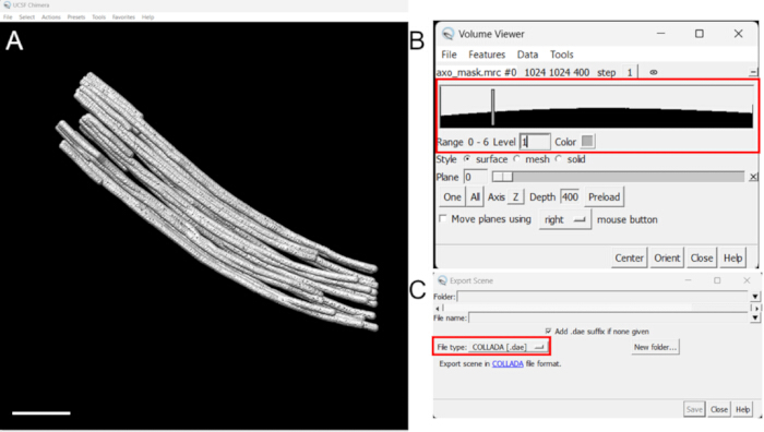
Figure 1: Exporting segmented cellular structures from Chimera. (A) Three-dimensional segmentation of T. brucei flagellar axoneme microtubules, shown in grey and displayed in the Volume Viewer of UCSF Chimera. Scale bar: 200 nm. (B) Volume viewer dialogue showing the threshold adjustment slider used to visualize the segmented structures. The threshold control is highlighted with a red box. (C) Export Scene dialog used to export the segmentation as a COLLADA (.dae) file for import. The COLLADA export option is highlighted with a red box. Please click here to view a larger version of this figure.

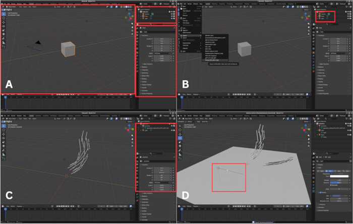
Figure 2: Importing segmented cellular structures. (A) Default workspace displayed after opening a new project. The top left box is the 3D Viewport, showing the current render environment. The top right is the Outliner, showing which objects are in the scene. The bottom left is the Properties panel, holding the settings for the objects and scene. (B) Import menu used for importing the exported segmentation file. The default objects included in a new Blender scene are highlighted in the red box and can be deleted before importing the segmentation data. (C) Imported segmentation of the 9 + 2 axoneme microtubules shown in grey. The imported segmentation appears as a new object in the scene, highlighted in the red box. The object scale and location can be adjusted in the object properties panel to bring the segmentation into a visible and manageable range. Note that the axoneme shown is not the same as the one from Figure 1. (D) Example of the imported segmentation after customization, including the addition of a ground surface, lighting, and texturing to improve visualization and prepare the animation. The Sun object is highlighted in the red box. The direction of the cast shadows is determined by the orientation of the Sun object, indicated by the diagonal line, rather than by its position in the scene. Please click here to view a larger version of this figure.

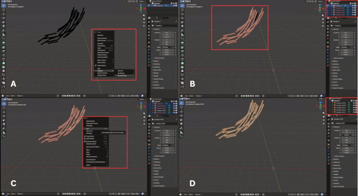
Figure 3: Separating and rejoining objects. (A) Separating objects in edit mode by using the Separate By Loose Parts option. (B) The result of separation. In the highlighted Outliner box, the new separated objects have been created. (C) Joining objects in Object view. All highlighted objects are joined together. (D) The resulting object is highlighted in Object view. In the Outliner, some leftover objects may still exist. These objects may be artifacts that can be safely deleted, or they may represent other sections of the data. Please click here to view a larger version of this figure.

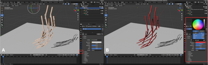
Figure 4: Applying materials to improve spatial depth perception and visual clarity. (A) Imported axoneme microtubule segmentation displayed with green material. The materials menu in the properties panel is highlighted with a red box. (B) The same segmentation after applying a distinct material with red coloring using the color wheel in the top right and a metallic sheen using the “metallic” setting. Adjusting material properties including base color, metallic value, roughness, and specular reflection, can enhance contrast, depth perception, and the visual separation of structural features in the three-dimensional model. Please click here to view a larger version of this figure.

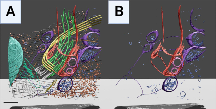
Figure 5: Representative visualization of segmented structures in the single-celled parasite Trypanosoma brucei flagellar base. (A) Full three-dimensional segmentation of the T. brucei flagellar base showing multiple cellular components, including axonemal microtubules (green), flagellar pocket membrane (red), four microtubules of the microtubule quartet (yellow), inter-vesicular membranes (purple), vesicles (blue and pink), ribosomes (orange), kinetoplast (light blue), basal body (white), and subpellicular microtubules (black). (B) Representative visualization of the same model after fading or hiding selected components to emphasize structures of interest. This approach allows users to reduce visual complexity and focus attention on specific regions or relationships within the tomographic segmentation. Scale bar: 200 nm. Please click here to view a larger version of this figure.

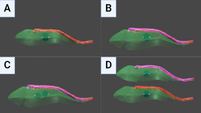
Figure 6: Animation of T. brucei cell division using an illustrative model. (A–D) Sequential frames from an animation illustrating cell replication and organelle separation in T. brucei. The cell body is shown as a transparent green model, with the parental flagellum shown in red and extending from the flagellar pocket. The emerging daughter flagellum is shown in magenta to distinguish it from the parental flagellum. The nucleus is represented as a dark blue metaball object. By adjusting object visibility, transparency, and position over time, complex cellular processes such as organelle duplication, segregation, and cell division can be illustrated in a clear and visually accessible format. Please click here to view a larger version of this figure.

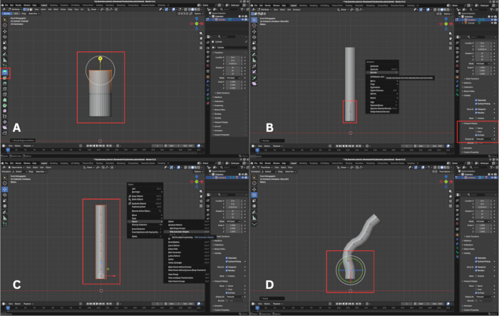
Figure 7: Creating an armature rig for model deformation. (A) A simple cylinder model is extended upward using the Extrude Region tool, highlighted on the left. The highlighted upper vertices of the cylinder are selected to define the region for extrusion. (B) An armature is built to fit the shape of the object. Similar to panel A, each bone is extruded from the last to create a skeleton that follows the entire length of the object. The armature is positioned inside the cylinder and displayed in front of other objects using the In front option in the Outliner highlighted in the bottom left. (C) The armature is fixed to the object using the With Automatic Weights option. Select the object first, then select the armature before parenting. (D) Example of model deformation after rotating the armature bone. During rigging, deformation occurs through the displacement of vertices influenced by the rotation of nearby bones. Therefore, smoother and more fluid animations require sufficient vertices to work within the mesh. Multiple bones can be extruded from a single starting bone or branching point to generate more complex or localized movements, depending on the shape and motion required for the model. If the model does not bend as expected, manually adjust bone weights or further subdivide the mesh to improve deformation. Please click here to view a larger version of this figure.

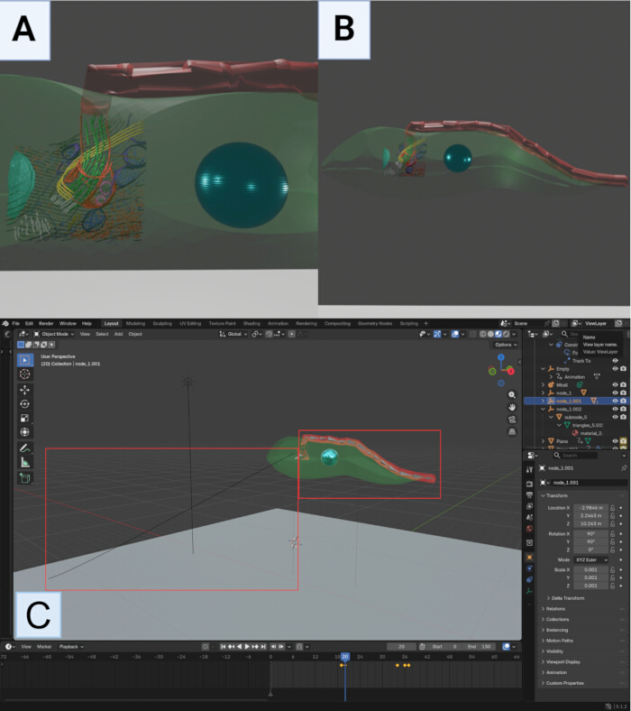
Figure 8: Integrating tomographic segmentation with an illustrative cellular model. (A) Close-up view of the segmented flagellar base positioned within the illustrative T. brucei cell model generated. The segmentation is placed near the flagellar base region to show its approximate location within the cellular context. (B) Wider view of the combined model, showing the segmented flagellar base in relation to the cell body, nucleus, and flagellum. This integrated visualization allows experimentally derived ultrastructural information to be presented within a whole-cell framework. During animation, the camera can move from a close-up view of the segmentation to a broader view of the cell, helping viewers understand both the structural details and their spatial relationship to the larger cellular architecture. (C) The interface of the final rendered animation. The left red box highlights the camera path used to move from the interior view of the cell shown in panel (A) to the wider whole-cell view shown in panel (B). The right red box highlights the illustrative cell in green and the flagellum model in red, including the rigging elements of bones used to position and rotate the flagellum along the cell body. Please click here to view a larger version of this figure.

Supplementary Video 1: Exporting segmentations from Chimera using flagellar microtubules as an example.Please click here to download this file.

Supplementary Video 2: Importing segmentations using flagellar microtubules as an example.Please click here to download this file.

Supplementary Video 3: Separating and joining segmentation objects using a flagellum as an example.Please click here to download this file.

Supplementary Video 4: Preparing the sample environment by adjusting lighting and coloring objects, using a flagellum as an example.Please click here to download this file.

Supplementary Video 5: Example visualization of a cryo-ET reconstruction and segmented 3D model of the flagellar base for animation. Please click here to download this file.

Supplementary Video 6: Visualization of an intact dividing Trypanosoma brucei cell model created in Blender for integration with cryo-ET segmentations.Please click here to download this file.

Supplementary Video 7: Integrated visualization of cryo-ET segmentation of the flagellar base within an illustrative Trypanosoma brucei cell model.Please click here to download this file.

Diskussion

This protocol provides a workflow for importing models from Chimera into Blender to generate high-quality scientific visualizations and animations. While the initial steps for preparing, exporting, importing, scaling, and organizing the segmentations are essential for maintaining a manageable and reproducible workflow, once the segmentations are imported, the workflow remains flexible, allowing users to customize segmentation presentation, material properties, lighting, camera movement, and scene composition according to the needs of biological questions.

In addition to rendering segmented structures, Blender also allows users to create illustrative cellular models that can be combined with experimentally derived segmentations. This capability is particularly useful for placing cryo-ET data within a broader cellular context. For example, segmented flagellar structures can be positioned within an illustrative whole-cell model to show their approximate location and spatial relationship to surrounding cellular features. By integrating data-derived segmentations with illustrative models, researchers can communicate complex structural information more clearly and effectively through scientific movies.

A major advantage of using Blender is its animation-focused design and open-source accessibility. The software provides extensive tools for mesh editing, material assignment, lighting control, camera movement, and rendering. Although this protocol focuses on elementary tools needed to animate segmented cryo-ET data and illustrative models, many additional functions can be explored to further improve the quality and complexity of the final visualization. For users new to Blender, foundational documentation and publicly available tutorials offer useful guidance on basic rendering concepts, including modeling, texturing, lighting, camera control, and animation. In addition, third-party add-ons have been created specifically for scientific visualization, including tools such as “Microscopy Nodes” for visualizing high-dimensional microscopy data⁹. These resources highlight the versatility of the Blender software and its ability to support a range of scientific visualization workflows while preserving spatial and temporal relationships within complex datasets.

Despite the benefits, several limitations should still be considered when using Blender for scientific visualization. Rendering high-resolution movies can be computationally demanding, particularly when working with complex segmentations, detailed illustrative models, high-quality lighting, or transparent materials. These tasks may require substantial random-access memory, graphics processing power, and rendering time. Depending on the available hardware, users may need to balance model complexity, visual quality, and render efficiency to avoid slow performance or software crashes. Blender includes two main render engines: EEVEE for real-time rasterization, and Cycles for physically accurate raytracing. Although Cycles can generate more photorealistic renders and improve depth perception without requiring a GPU, EEVEE may be preferable because of its faster rendering speed and relatively minor quality trade-offs for segmentation renders. The figures and supplementary videos presented in this protocol were produced using a workstation with a 64-core processor, 512 GB RAM, and dual NVIDIA RTX A5500 GPUs, allowing the animation to be rendered within a few minutes. However, this hardware configuration exceeds the minimum requirements needed for elementary visualization workflows. For users with more limited computational resources, reducing model complexity, simplifying materials, lowering viewport quality, or using a faster rendering engine can improve performance. The minimum hardware specifications for Blender are provided in the Table of Materials.

During editing or rendering, users may encounter issues that slow performance or hinder the work. We recommend closing other memory or RAM-intensive programs before importing or rendering segmentations, and saving the project frequently. If the interface becomes slow, reducing viewport shading quality in the top right will help reduce the strain before rendering. If the render view doesn't update properly, users can adjust the animation quality settings in the Output section in the bottom left window, such as Pixel Density, or Output Quality and Encoding Speed in the Video tab, before exporting the final movie.

It is important to distinguish experimentally derived segmentations from illustrative or modeled components. Segmentations imported from cryo-ET data represent structural observations, whereas illustrative cellular models, deformations, and simulated movements are visual aids. Animations involving resizing, repositioning, or deformation should therefore be interpreted as conceptual representations rather than direct measurements from the tomographic data. Clear visual labeling, consistent color schemes, and careful description of the modeled elements can help avoid misinterpretation.

In summary, using Blender provides a flexible and powerful platform for transforming cryo-ET segmentations into scientific animations. Although users may encounter challenges related to computational resources, rendering time, and the learning curve for three-dimensional modeling, the benefits for scientific visualization are substantial. By combining tomographic segmentations with customizable rendering, camera control, and illustrative modeling, one can enhance the communication of complex cellular structures and biological processes.

Materialien

Liste der in diesem Artikel verwendeten Materialien

Name	Unternehmen	Katalognummer	Kommentare
Aquilos 2 Cryo-FIB	Thermo Fisher Scientific	1210685	cryoET lamella generation instrument
Blender Software	Blender Foundation	Version 5.2	Minimum specs: 4 core CPU, 8 GB RAM, 2 GB VRAM GPU
EMAN2	Baylor College of Medicine	Version 2.99
Falcon 4i Direct Electron Detector	Thermo Fisher Scientific	https://www.thermofisher.com/in/en/home/electron-microscopy/products/accessories-em/falcon-detector.html
IMOD	University of Colorado, Boulder	Version 4.8.50
MotionCor2	University of California San Francisco	Version 1.6.5a
Relion 3.1	MRC Laboratory of Molecular Biology	Version 3.1
Selectris Imaging Filter	Thermo Fisher Scientific	https://www.thermofisher.com/in/en/home/electron-microscopy/products/accessories-em/selectris.html
Titan Krios Cryo-TEM	Thermo Fisher Scientific	https://www.thermofisher.com/in/en/home/electron-microscopy/products/transmission-electron-microscopes/krios-cryo-tem.html
Tomography 5 Software	Thermo Fisher Scientific	PN 307499
UCSF Chimera	University of California San Francisco	Version 1.16